Detection Algorithm of Audiovisual Production Invariant Siba Haidar1 , Philippe Joly1 , and Bilal Chebaro2 1
´ IRIT, Equipe SAMoVA, Universit´e Paul Sabatier, Toulouse, France
[email protected],
[email protected] 2 Universit´e Libanaise, Facult´e de Sciences, section 1, Liban
[email protected]
Abstract. In video documents, the style signature extraction is a highly interesting process since it provides a new feature for contents classification. This paper defines what we call production invariants and proposes an algorithm for detecting them through out a collection of multimedia documents. The algorithm runs on audiovisual features, considered as time series, and extracts invariant segments using a one-dimensional morphological envelop comparison in a dichotomic approach. The audiovisual production invariants are then determined after the fusion of results obtained on a large set of low-level features.
1
Introduction
Video feature extraction is used for segmenting, classifying and indexing video documents. Video content analysis is a first step before applying information retrieval and browsing tools in order to satisfy some queries on audiovisual content. In this paper, we introduce a new analysis tool for indexing and classification of multimedia contents, called “Audiovisual Production Invariants” which are the elements that constitutes semantic document signature. We show that the tool’s construction relies on the low-level document features. We propose a simple algorithm to detect the tool’s elements. The detection algorithm requires neither any previous knowledge about the features natures and behaviors, nor user intervention in order to define or change thresholds, to produce a result. This permits its application on different types of audiovisual documents and different kinds of low-level features. The organization of the paper is as follows. In section 2, we define audiovisual production invariants and highlight their interest for automatic audiovisual analysis. In section 3, we present our comparison algorithm used to extract similar segments from low-level features seen as time series. We then show how to represent results obtained from each feature in order to make data fusion and detect audiovisual invariants (section 4). An illustration of our approach will be shown in the results in section 5. Finally, section 6 concludes with some key points for futur works.
2
2
Audiovisual Production Invariant
Video documents may have very different characteristics and properties. However, we all agree that there are some common points between all political programs, or all football matches, or, time to time, between all the movies realized by a given director. These common points are what we call invariants. 2.1
Definition
A production invariant, as we define it, is what characterizes a document or a set of documents belonging to a same “collection”, of a same director, or produced following the same set of guidelines. To localize and extract a production invariant, we rely on the set of all possible features characterizing an audiovisual document [1] which can be extracted and quantized to build numeric time series. We consider that production invariants will appear, in audiovisual documents, as the repetition of the same sequence of values of different low-level features extracted from two different streams or two different parts of a same stream, and more generally of a stream collection. In other words, the invariant is a segment, seen as common- or similar- or even as a repetitive sequence of values, from the point of view of one or multiple features. The size of these schemas may vary, and all the extracted features are not necessarily involved in the expression of these sequences. For example, a production invariant can be the iteration of some specific values when the anchor frame appears in a TV News program, or at the beginning of a same game show broadcasted on two different days. In this context, and in order to detect invariants, we need to determine whether two given features (or more exactly their time series) display a similar behavior at a certain moment. The problem is interesting (and difficult) because, unlike traditional tools for audiovisual content querying, we do not have, a priori, a sample model of what we are looking for. This means that we do not know previously what we are searching for, where it can be or even what dimension or length it may have. 2.2
Interest
Production invariants will be extracted by the analysis of different programs of a same collection. Once they are determined after this learning step, they are useful in various operations for documents’ semantic analysis. For instance, production invariants will be easily detected in any document of a same collection, or eventually be used to automatically detect an occurrence of an item of this collection. Even more, since invariants characterize video segments, they can be used later to identify or localize them. Another benefit we can see in invariants, is the validation of production charts, i.e., a director can use them to follow up the evolution of his realizations and see whether or not they do apply his rules and guidelines.
3
Thus, the use of extracted video features to find what could be production invariant, relative to a given set of video document offers a new tool in scenes classification and ToCs (Table of contents) and Index creation.
3
Multi Level Analysis Matching Using Morphological Filtering
Since we propose a new algorithm for comparing two time series, we quickly describe similarity measures and indexing techniques that have been proposed for time series analysis. Then we introduce our new algorithm for invariant segments extraction based on dichotomous division and morphological one-dimensional envelope comparison. 3.1
Time Series Similarity Measures
The main idea behind similarity measures is that they should allow imprecise matches. There are several applications of such measures. For example, they can be used to cluster the different time series into similar groups, or to classify a time series based on a set of known examples. Another point of interest is the indexing problem which can be formalized as: “given a set of time series Q, prepare an index offline such that given a query series q, the time series in Q that are most similar to q can be reported quickly” [2]. All similarity measures intend to bypass obstacles, such as the subsequence similarity problem, the rule discovery problem, and clustering problems, which have to be overcome in our approach. Furthermore, we consider that, as well as accuracy, efficiency (in terms of computational cost) is a challenging issue. Dynamic time-warping based matching (DTW) is a popular technique in the context of speech processing [3], sequence comparison [4], and shape matching [5]. This method has been used to match a given pattern in time-series data. The essential idea is to match one dimensional pattern while allowing local stretching of the time parameterization. It is a robust measure that allows non-matching gaps, amplitude scaling, and offset translation. Longest Common Subsequence (LCSS) Measures are based on the edit distance [6][7] and work on sequences with slightly different length. It considers two sequences to be similar if they have enough non-overlapping time-ordered pairs of subsequences that are similar. The algorithm consists in finding all atomic similar subsequence pairs, which is achieved by a spatial self-join over the sets of all atomic windows. 3.2
Recursive Quadratic Intersection
The DTW and LCSS time series similarity measuring methods referred to in the previous section, are well known techniques dealing with imprecise data. However the huge length of time series we will have to handle requires a simpler
4
and faster similarity measure applicable on all time series natures. That is why we choose the morphological operators in measuring similarity [8]. Also, most of the similarity measures proposed in the domain of time series do not intend to merge the result of multiple comparisons. They are supposed to be applied on one type of time series at a time. Thus, parameterization issue is not a problem for them; it can be fixed once at the beginning of the process depending on the type of studied time series. In our case, a production invariant is identified after combining all studied features results. As we will show, features extracted from an audiovisual document do not have a comparable evolution. For example, we have defined a measure of the color contrast which is obtained here by iteratively measuring the distance between the two main dominant colors, given by the following formula: contrast = |L1 − L2 | + distcirc (H1 , H2 ) × log
¡S
1 +S2
2
¢
(1)
where L1 , L2 are respectively the luminance of the two dominant colors, H1 , H2 the hue, and S1 , S2 the saturation, and where distcirc (x, y) is the circular distance between x and y, knowing that x and y vary inside certain boundaries.
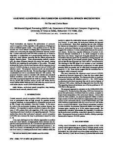
This feature is very noisy and eventful (figure 1.b), and presents many peaks. On the contrary, a feature with a very different behavior is the mean luminance (figure 1.a), which calculates the average of pixels’ luminance in each frame, and which is very smooth. As it appears in figure 1, no normalization was applied on features, because until now, all applied operators are relative to each feature and so there is no meaning of a scale comparison.
Mean luminance (0:500)
Contrast (0:500)
250
2000
1800
200
1600
1400
MeanLuminance
150
Contrast
1200
1000
100
800
600
50
400
200
0
0
50
100
150
200
250 300 time progress
(a)
350
400
450
500
0
0
50
100
150
200
250 300 time progress
350
400
450
500
(b)
Fig. 1. This figure shows the mean luminance feature smoothness (a) compared to the eventful color contrast feature (b). Both are extracted from the same audiovisual segment
5
Considering this fact, we expect our algorithm to be independent from the feature behavior; the comparison algorithm is applied uniformly on all the time series, despite their smoothness. Also, we allow no smoothing considering that peaks carry important information related with an event in the video, like a lightning effect or a sudden movement or even a view or a scene change (see figure 2). In general, only a few peaks may be due to noise.
Motion Rate (0:1000) 3500
3000
2500
Motion Rate
2000
1500
1000
500
0
0
100
200
300
400
500 600 Time Progress
700
800
900
1000
Fig. 2. Meaningful peaks in the motion rate feature curve; they announce scene changes. They are either sudden peaks designating a cut transition, or progressive variations when occurs a cross-dissolve
Our sequence matching method, like most of the matching methods, in an environment with a large set of data sequences, works in two phases. – In the first phase, only a finite number of data sequences are kept after a filtering process. We consider that these sequences are matching candidates. – In the second phase, all candidate sequences are verified for the actual matching using a morphological filtering comparison filter. Definition 1. Matching sequences: Two sequences of length l are considered to be similar if their covering similarity measure bypasses a certain threshold. Definition 2. Covering: The covering is the percentage of sub-sequences associated by the morphological coupling process. It is given by the following formula: covering (Ii , Jj ) =
nbCoupledSubsequences(Ii ,Jj ) nbTotalSubsequences(Ii ∪Jj )
(2)
where nbCoupledSubsequences is the number of sub-sequences of similar morphological envelop.
6
The choice of the covering similarity threshold depends on the accuracy requested for the similarity measure. The algorithm proceeds in a dichotomous approach in order to avoid useless comparisons. No continuation in depth is made unless suspected resemblance is possible. We introduce here the algorithm we call the Recursive Quadratic Intersection (Algo.1). Algorithm 1: RQI step 1 RQI(a,b,t) { % a & b equal length of power of 2 % t is the desired length of candidates also power of 2 if [min(a),max(a)] intersects [min(b),max(b)] if length(a)>t & length(b)>t divide equally a into a1 and a2 divide equally b into b1 and b2 RQI(a1,b1,t) RQI(a2,b1,t) RQI(a1,b2,t) RQI(a2,b2,t) else add (a,b) to potentialCandidates return potentialCandidates } The result is a set of candidate intervals R all of which have the requested length t. Refer to figure 3 for sample candidate sequences. R = {(Ii , Jj ) /Ii ⊂ a, Jj ⊂ b ∧ Ii ∩ Jj 6= φ ∧ length (Ii ) = length (Jj ) = t} (3)
3.3
Similarity Measure Using Morphological Envelops
Once potential candidates are filtered, given two sequences, we shall proceed to the resemblance verification with the covering measure. To achieve this, we construct a one-dimensional morphological envelope using erosion and dilation, and a structuring element of size α on each couple (Ii , Jj ) . The value of α is determined proportionally to t in order to preserve the global shape of the curve - time series representation - but not the small fluctuations (Algo. 2). In our experiments we vary alpha around 3% of t. Algorithm 2: RQI step 2 verifySimilarity(Ii,Jj,alpha) { % alpha is the morphological filter if covering(Ii,Jj,alpha)> P
7
225 220
220
215
210
215
205 210
200 205 195
200
900
920
940
960
980
1000
1020
4620
4640
4660
(a)
4680
4700
4720
(b)
1800
1800
1600 1600
1400 1400
1200 1200
1000
800
1000
600 800
400 600
200 4.116
10
4.117
10
4.118
10
4.119
10
4.12
10
(c)
4.121
10
4.122
10
4.123
10
4.124
10
3.11
10
3.12
10
3.13
10
3.14
10
3.15
10
3.16
10
3.17
10
3.18
10
(d)
Fig. 3. Samples of potential candidate sequences filtered by the RQI algorithm in a first step. a and b are for mean luminance feature, c and d for motion rate feature
8
add (Ii,Jj) to similarCandidates return similarCandidates } covering(Ii,Jj,alpha) { if length(Ii)&length(Jj) tMax) divide equally a into a1 & a2 divide equally b into b1 & b2 for each couple (ai,bj) compare(ai,bj) %4calls } compare(x,y) { if potentiallySimilar(x,y) verifySimilarity(x,y) else if length > tMin divide by two: x1,x2,y1,y2 compare(xi,yj), } In our experiments, we have fixed for t a minimal value of 1 second, and a maximal one of 42 seconds, which is not the longer subsequence we can extract but the maximum length to which applying the similarity measure still has sense. Next in the matrices representation, we show that similar segments of longer length will be gathered by a simple process. The RQI algorithm introduced in this section works on deep down comparison. It continues to compare until it finds all possible similar segments of different lengths. Note that many operations will be avoided due to an empty intersection checked before further going deep down. We obtain variable length couples judged as similar for the considered feature. In the next paragraph, we present how we use these couples and how we filter significant ones based on the fusion of multi-characteristic results.
10
4
Invariant Features Fusion
The result of the RQI algorithm, when applied to one feature, i.e. one time series, can be viewed as the union V S of several sets each of which has the form of S for a certain scale t, equation 5. V Sf eaturex =
o StM ax n covering(Ii ,Jj )≥P ∧ (I , J ) ∈ (a, b) / i j tM in length(Ii )=length(Jj )=t
(5)
After the application on all the extracted audiovisual features, we obtain as many sets as the number of features. In this case, the result will need to be filtered. Only pertinent information will be kept. The filtering process and the fusion of all results belong to the domain of data fusion since we totally follow its definition in [9] which is: “data fusion is a formal framework in which are expressed the means and tools for the alliance of data originating from different sources”, and “data fusion aims at obtaining information of greater quality;”, “it may also be related to the production of more relevant information of increased utility”. In our case, this “more relevant information of greater quality” is the production invariants which are document’s invariant segments resulting from the fusion of low level features’ invariant segments. 4.1
Invariant Segment Representation
We present results obtained by the RQI algorithm by a square matrix as in figure 5, of dimension n =length(a) /tM in. Arrows labelled a(document1) and b(document2), means that we are comparing the feature Fx for two different documents of length n. The extraction of this feature x from the documents 1 and 2 is time series a and b. Rates cij filling the matrix are sequences covering values obtained by similarity verification. Each diagonal k of the matrix represents the resemblance between these documents for the feature Fx , for a certain alignment. Diagonal zero shows the parallel alignment of the two time series. According to formula 5, couples (Ii , Jj ) in V Sx , depending on their length t, will be represented as t/tM in points of rate cij = P . We read this couple as the quadruple (i1, i2, j1, j2). 4.2
Production Invariant Detection Based on Voting Method
A first step in this multi-feature data fusion will be the arithmetic fusion taking into account rates cij. In this paper, we suppose that all features are totally dependant of the audiovisual segment from which they are extracted, i.e., beside usual noise and experimental errors, features do not represent random data. This fusion method decides whether or not segments are invariants to all features, we have then for the moment just one class: the invariant class.
11
Fig. 5. Matrices representation
4.3
Production Invariant Classification
Classification and interpretation of the fusion result matrix is very easy. We can localize invariants and classify them using their scores and length. Therefore, it is necessary to consider the following cases: – first, in general, one tiny common segment is meaningless unless a large number of features says the contrary, i.e. it has a high rate, – then, a large segment (Ii , Jj ), said to be invariant, even with only a few number of features (it can be one feature) is most probably a production invariant.
5
Preliminary Results
One concrete example of production invariants we were able to extract after combining results for several features, is the credits extraction without previous model in hand or learning phase. All the features agreed on the invariant property of the credits of a TV game show because it is automatically sent on the beginning of each transmission. It means that we succeeded to catch this invariant despite the noise effects on transmission. The credits evolution is quickly shown in figure 6. In figure 7, we can see a subset of the curves - corresponding to graphical representation of extracted
12
Fig. 6. An invariant production for a game show: credits
250
250
200
200
150
150
100
100
50
50
0
100
200
300
(a)
400
500
600
0
100
200
300
400
500
600
(b)
Fig. 7. Representation of the feature evolutions used to detect TV game credits for each document
13
features as time series - which are relative to the credits of this TV game program (between the vertical bars), broadcasted on two consecutive days. Another production invariant extracted from another couple of recordings is the weather newscast which is always present after the TV news program. (figure 8) In this invariant, many features, such as those concerning motion and color, had the same evolution during a long segment of time. For the time being, we are using low-level video and image features in our experiments. Audio features will be added in future works.
250
250
200
200
150
150
100
100
50
50
0
0
50
100
150
200
250
300
350
400
450
500
0
0
50
100
150
200
250
300
350
400
450
500
Fig. 8. The weather newscast and corresponding features representation
6
Conclusion and Future Works
We proposed a method for production invariant extraction from video sequences. The method is based on a hierarchical comparison approach using morphological filtering. Given two audiovisual documents, we used fast search techniques able to extract all similar subsequences, of different lengths, and this for each feature characterizing the document. We have introduced the idea of combining multiple subsequence comparison, of features extracted from audiovisual documents, in order to filter significant results. We call those results production invariants.
14
Later, in order to improve the robustness of invariant extraction, we will combine criteria on the base of audiovisual rules. We will use methodological data fusion strategy. Among the various strategies for data fusion, we can find: arithmetic methods, statistics methods, fuzzy logic and possibility methods (adaptive method), and evidence theory fusion. Each of these methods depends on a point of view [10]. We will also, study the interest of applying confidence indexes as used by Gutierrez et al. in [11] to discriminate results from features according to their reliability. Acknowledgement This work has been conducted on the behalf of the KLIMTITEA project and in the PIDOT-CNRS framework.
References 1. Adami, N., Corvaglia, M., Leonardi,R.: Comparing the quality of multiple descriptions of multimedia documents. MMSP 2002 Workshop, St. Thomas, US Virgin Islands, (2002) 2. Gunopulos, D., Das,G.: Time Series Similarity Measures. Sixth ACM SIGKDD International Conference on Knowledge Discovery and Data Mining, Boston, MA, USA, (2000) 3. Sakoe, H., Chiba, S.: Dynamic programming algorithm optimization for spoken word recognition. IEEE transactions on Acoustics, Speech and Signal Processing, (1978) 4. Erickson, B. W., Sellers, P. H.: Recognition of patterns in genetic sequences. Time Warps, String Edits, and Macromolecules: The Theory and Practice of Sequence Comparison. Addison. Wesley, MA, (1983) 5. McConnell, R.: Correlation and dynamic time warping: Two methods for tracking ice floes in SAR images. IEEE transactions on Geosciences and Remote Sensing, (1991) 6. Bozkaya, T., Yazdani, N., zsoyoglu, M.: Matching and Indexing Sequences of Different Lengths. Conference on Information and Knowledge Management, Proceedings of the sixth international conference on Information and knowledge management, Las Vegas, USA, (1997) 7. Ganascia, J-G.: Extraction of syntatical patterns from parsing trees. JADT 2002 : 6es Journ´es internationales d’Analyse statistique des Donn´ees Textuelles. (2002) 8. Serra, J.: Outils de morphologie mathmatique pour le traitement d’images. Centre de Morphologie Math´ematiques, Ecole des Mines de Paris, Fontainebleau, (2000) 9. http://www.data-fusion.org, 10. http://www.survey.ntua.gr/main/labs/rsens/DeCETI/IRIT/MSIFUSION/index.html, 11. Gutirrez,J., Rouas, J.-L., Andr-Obrecht, R.: Fusing Language Identification Systems using Performance Confidence Indexes. International Conference on Acoustics, Speech and Signal Processing, Montreal, May (2004)