Detection and Isolation of Oscillations Using the ...

Author's accepted manuscript, published in Conference on Control and Fault Tolerant Systems, 2010, France

Detection and Isolation of Oscillations Using the Dynamic Causal Digraph Method Vesa-Matti Tikkala, Alexey Zakharov, Sirkka-Liisa J¨ams¨a-Jounela Abstract— This paper proposes a modification to the dynamic causal digraph (DCDG) method in order to address the detection and isolation of oscillations in a process. The proposed detection method takes advantage of the properties of residual signals generated by the DCDG method by studying their zerocrossings. The method is tested in an application to a board making process and the results are presented and discussed.

I. I NTRODUCTION Demands to keep industrial processes running efficiently with a high rate of utilization are increasing constantly due to the tightening global competition. Since, the modern industrial processes are complex and large-scale, operatorbased monitoring cannot guarantee early enough detection and reliable diagnosis of the faults and abnormalities. Therefore, the detection and diagnosis of different abnormal and faulty conditions in the processes have become increasingly important. Common problems causing inefficient operation and production losses in the process industry are oscillations. Oscillatory disturbances readily propagate in the process and cause extensive variation in the process variables. The oscillations are usually originated under feedback control, and they may have various causes which have been categorized by Thornhill and Horch into non-linear and linear causes [1]. Nonlinear causes include for example extensive static friction in the control valves, on-off or split range control, sensor faults, process non-linearities and hydrodynamic instabilities. The most common linear causes are poor controller tuning, controller interaction and structural problems involving process recycles [1]. According to Choudhury et al. , valve stiction is, however, the most common cause of these oscillations in control loops [2]. The detection and diagnosis of oscillations have been previously addressed by data-based methods which study, for example, the properties of controller error signals [3], [4], the spectral properties [5] or the nonlinearity of the measurement signals [6], [7]. Also, a variety of multivariate methods, such as principal component analysis [8] and nonnegative matrix factorization [9], have been applied to solve this diagnosis task. A recent trend has been to introduce process information into the diagnosis of plant-wide oscillations. Applications in which the process connectivity information has been integrated into data-based analyses to check hypotheses on the fault origin, have been presented [10], [11].

This paper aims at further development of the dynamic causal digraph (DCDG) method by addressing the detection and isolation of plant-wide oscillations. A detection algorithm, which is able to deal with oscillatory residuals, is proposed and integrated into the DCDG method. In this paper, the modified DCDG method is used to detect and isolate low-frequency oscillations caused by a valve stiction fault in a board machine process. The paper is organized as follows. In Section II, the dynamic causal digraph method and the new detection algorithm are introduced. The process and the test environment are described in Section III. The results of the testing are presented in Section IV followed by the conclusions in Section V. II. E NHANCED DCDG M ETHOD FOR THE D ETECTION AND I SOLATION OF O SCILLATIONS The dynamic causal digraph method employs the process knowledge formalized as a causal digraph model in order to perform the ordinary fault diagnosis tasks as presented in [12], [13]. In the enhanced DCDG, the detection of faults is performed using the proposed method which observes the zero-crossings in the residuals generated by a comparison of cause-effect models and the process measurements. Next, the isolation is carried out by applying a set of inference rules to the residuals in order to extract the fault propagation path. Finally the arcs in the digraph that explain the faulty behavior are identified. The enhanced DCDG method is described in more detail in the following. A. Fault detection Fault detection is performed in two steps: residual generation and fault detection in the residuals using the modified cumulative sum (CUSUM) algorithm. 1) Residual generation with dynamic models: The dynamic causal digraph produces two kinds of residual to be used in fault detection and isolation: global (GR) and local residuals (LR). The global residual is produced from the difference between the measurement and the global propagation value: GR(Y ) = Y (k) − Yˆ (k),

(1)

where Y (k) is the measurement and Yˆ (k) is the global propagation value obtained by   ˆ (k − 1), U ˆ (k − 2), . . . , Yˆ (k) = fY U (2)

where fY is a discrete-time model describing the causeeffect relationship from n predecessor nodes Ui to node Y .

978-1-4244-8154-5/10/$26.00 ©2010 IEEE

ˆ (k − τ ) = {ˆ U u1 (k − τ ), . . . , u ˆn (k − τ )} are the lagged global propagation values from the predecessors with time lags τ = 1, 2, . . . depending on the system order. The local residuals are subcategorized into three types: individual local residuals (ILR), multiple local residuals (MLR) and total local residuals (TLR) [14]. The individual local residual is produced by taking the difference between the measurement and the local propagation value with only one measured input, while all the others are propagation values from the parent nodes:

where

ILRYm = Y − Y¯ ,
¯ (m, k − 1), U ¯ (m, k − 2), . . . , Y¯ (k) = fY U

¯ (m, k − τ ) = U

u ¯i (k − τ )

(3)

(

( u ˆi (k − τ ), i 6= m u ¯i (k − τ ) = ui (k − τ ), i = m

)

,1 ≤ i ≤ n ,

(4)

u ˆi (k) is the lagged global propagated value from the predecessors, and ui (k − τ ) is the measurement for the i-th parent node. Pl Similarly, the M LRY Y is produced as l

P (5) M LRY Y = Y − Y¯ ,
l l ¯ ¯ ¯ Y (k) = fY U (PY , k − 1), U (PY , k − 2), . . . ,

where

¯ (PYl , k − τ ) = U

u ¯i (k − τ )

(

( ) u ˆi (k − τ ), i ∈ / PYl u ¯i (k − τ ) = ,1 ≤ i ≤ n , ui (k − τ ), i ∈ PYl

(6)

where max{·}-operator takes the maximum of its arguments, 2 ¯ ∆t(k) and σ∆t (k) are the mean and the variance of the time between consecutive zero-crossings in a residual, respec¯ and σ 2 are calculated in a moving window tively. Both ∆t ∆t of length l: [e(k − l), e(k)], where e(k) is the residual. In normal operation, when the residuals are assumed to ¯ σ 2 (k) ≈ 2, since the be zero-mean Gaussian noise, ∆t, ∆t probability of e(t) having a different sign than e(t−1) is 0.5 for all t. Therefore, the nominal mean value of the observed signal in (7) can be set as µ0 = 2 and β and λ are then tuned to obtain robust detection with minimal false alarms. The window length l must be selected to be larger than one half of the expected period in the residual. B. Fault isolation 1) Isolation of the fault propagation path: Fault isolation is performed recursively for the detected nodes by using a set of rules. These isolation rules, developed by Montmain and Gentil in [14], are converted into a table for the convenience of implementation, as shown in Table I. After the isolation the nature of the fault is determined by using rules in Table II. TABLE II FAULT NATURE RULES OF THE DYNAMIC CAUSAL DIGRAPH CU (GR(X))∗ CU (T LR(X)) 1/-1 1/-1 1/-1 0 0 1/-1 ∗

PYl

is the set of indices of the predecessors which use the measurement as an input. The T LR(Y ) is produced with PYl = PY , where PY is the set of indices of all the predecessors of Y . The residual generation scheme follows the DCDG method developed in [14]. 2) Fault detection using the modified CUSUM method: The proposed detection method utilizes the cumulative sum (CUSUM) method presented in [15], by applying it to the detection of a change in the mean and variance of the zerocrossings in the residual signals. The CUSUM algorithm is defined for a positive change as follows: U0 = 0 n X β Un = d(k) − µ0 − , 2

where λ is a design parameter, usually tuned according to the requirements for the false alarm and missed alarm rates. The signal observed by the CUSUM algorithm, called the detection signal, is defined as follows   2 σ∆t (k) ¯ d(k) = max ∆t(k), , (8) ¯ ∆t(k)

(7)

k=1

mn = min Uk , 0≤k≤n

where β is a user-specified minimum detectable change, d(k) the observed signal with nominal mean value equal to µ0 . Whenever Un − mn > λ, a change is detected,

Fault nature Local fault for that child node Process fault for the faulty node Measurement fault for the faulty node

X is the subscript of any child node of the node Y .

2) Isolation of the faulty process component: In the case of a process fault, in addition to locating the fault on the variables (nodes), locating it on the arcs is also desirable. However, the MISO structure of the digraph causes problems by generating multiple possible results as 2n − 1, n ≥ 1, where n is the number of input arcs of the fault origin node(s). In order to decrease the number of possible results, an inference mechanism between the arcs proposed in [16] is used. The inference mechanism is based on an inter-arc knowledge matrix M defined for node U as follows   1, if inconsistency in arc hU, ii MU (i, j) = (9) causes inconsistency to hU, ji   0, otherwise,

where i and j refer to the matrix rows and columns, respectively. Next, each set of suspected arcs is tested in order to determine whether the fault may be caused exactly by the current set of arcs. In order to do it the matrix M is

TABLE I FAULT ISOLATION RULES OF THE DYNAMIC CAUSAL DIGRAPH CU (GR(Y )) CU (T LR(Y )) CU (ILRY (m)) CU (ILRY (i)) CU (M LRY (P1 )) CU (M LRY (P2 )) 0 0 0 0 0 0 1/-1 0 0∗ 1/-1∗ 0∗ 1/-1∗ ∗∗ ∗∗ ∗∗ ∗∗ 1/-1 0 1/-1 1/-1 1/-1 0 1/-1

1/-1

1/-1

1/-1

1/-1

1/-1

Decision No fault Fault propagates from the parent node m Fault propagates from the nodes with subscript P2 Local fault on variable Y

∗

∀i 6= m, i ∈ PY , m ∈ P1 , m ∈ / P2 , PY is the set of subscripts of parent nodes of the node Y . ∗∗ ∀i, m, i ∈ PY , m ∈ PY , ∀P1 , P2 ⊆ PY .

multiplied with a vector representing the suspected arc set, which is defined as follows ( 1, if ARC(M, i) ∈ S, 1 ≤ i ≤ Na sv(i) = (10) 0, otherwise, where ARC(M, i) gives the arc corresponding to the ith row in the matrix M. S is the set of suspected arcs. If the number of non-zero elements of sv have changed, the current suspected set of arcs must be excluded. III. D ESCRIPTION OF THE P ROCESS AND THE VALVE S TICTION FAULTS This test focuses on the stock preparation of the board machine at Stora Enso’s mills in Imatra, Finland. The simulation tests are run on a board machine simulator model in the APROS simulation environment.

TABLE III VARIABLES OF THE CAUSAL DIGRAPH MODEL FOR THE STOCK PREPARATION OF THE BOARD MACHINE . Var. Description vb valve opening for the broke line fb mass flow of the broke vbd dilution water valve opening for the broke line f bd dilution water flow for the broke line cb broke consistency rp pine pump rotation speed fp mass flow of the pine stock vpd dilution water valve opening for the pine line cp pine consistency rc CTMP pump rotation speed fc mass flow of the CTMP vcd dilution water valve opening for the CTMP line cc CTMP consistency vmcd dilution water valve opening for the machine chest cmc consistency before the machine chest pp pressure before the pine valve pc pressure before the CTMP valve ct consistency of the machine chest A: Actuator signal, M: Measurement signal

Type A M A E M A M A M A M A M A M M M M

Unit kg/s kg/s % % kg/s % % kg/s % % kg/s kg/s %

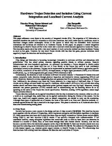
A. The Board Machine Process The board making process begins with the preparation of raw materials in the stock preparation section, as shown in the flowsheet in Fig. 1. Different types of pulp are refined and blended according to a specific recipe in order to achieve the desired composition and properties for the board grade to be produced. The consistency of the stock is controlled with dilution water. The blended stock passes from the stock preparation to the short circulation. First, the stock is diluted in the machine chest to the correct consistency for web formation. The diluted stock is then pumped with a fan pump, which is used to control the basis weight of the board, to cleaning and screening. Next, the stock passes to the head box, from where it is sprayed onto the wire in order to form a solid board web. The excess water is first drained through the wire and later by pressing the board web between rollers in the press section. The remaining water is evaporated off in the drying section using steam-heated drying rolls. The variables used in the causal digraph model of the stock preparation are listed in Table III and the structure of the digraph model of the stock preparation section is presented in Fig. 2. B. Valve Stiction Faults A control valve is the most common final control element used in the process industry [2]. Therefore, the diagnosis of faults in valves is of great importance. Stiction, short for static friction, is a problem in control valves since it

rc

fc

vmcd

pc vcd

cc

rp

fp

cmc

ct

pp vpd

cp

vb

fb

vbd

cb

Fig. 2. Structure of the causal digraph model of the stock preparation section of the board machine

can cause significant disturbances in the process variables. A valve suffering from excessive stiction sticks when the control signal, for example, changes the direction and does not move until the force required to move the valve shaft exceeds a certain limit. When the valve starts to move, it jumps and then follows the control signal before it sticks again. A sticking valve is likely to cause oscillations when it is involved in a control loop. The stiction in valves has been modelled and studied e.g. in [17] and [18]. This paper considers a stiction fault in a pressure control valve which causes the control loop to oscillate and disturbs the operation of the plant.

Dilution water

Pine chest

Dilution water CTMP chest

,........,................................................ I

II(LC

Broke chest

Fig. 1.

Flowsheet of the stock preparation of the board machine process.

IV. TESTING AND RESULTS A. Simulation Environment and Fault Simulation The Imatra board machine model was developed by Stora Enso and VTT in the APROS environment. It was originally constructed on the basis of modeling and simulation studies carried out during 1998-2002 for Stora Enso's Imatra mills. It has been previously used for grade change simulations and in studies reported by Lappalainen et al. in [19]. A valve stiction fault was simulated in the stock prepa­ ration part of the board machine using the APROS board machine model. The faulty valve is located in the CTMP line and is used to control the feeding pressure P c of the blend chest. The two-parameter data-driven valve stiction model proposed by Choudhury et al. in [18] was implemented in the APROS simulation software for the simulation. The

100

Fig. 3.

200

300

400

500

600

700

800

900

Normalized process variables during the fault simulation.

deadband and slip-jump parameters of the stiction model were set to S

=

0.06 and J

=

0.06 respectively. That is,

the stiction is set to be 6% of the operation range of the

following: f3

=

10, >..

=

4 and I

=

200. The global residuals,

valve. The fault was evoked by a step change to the setpoint

detection signals and the detection results for variables

of Pc. The fault occurring at t

and =

100 causes an oscillation

Ie

Ce

are presented in Fig. 4. The fault is detected in both

signals

GR(fe) and GR(ce). The change in the detection (k) was detected for the first time at k 103, three

with a period of approximately 120 samples, which affects

signal d f

most of the variables in the stock preparation. Fig. 3 shows

time instants after the fault occurred. However, the detection

c

=

k

result is not reliable until

demonstrates clearly the effect of the fault in the process.

is detected later at

B. Fault Detection and Isolation Results

inference to isolate the origin of the fault. The local residual,

k

=

=

170. The global residual of

Ce

the measured variables during the fault simulation and it

215.

Local residuals were generated in order to carry out the First, the global residuals for all variables were produced

the detection signal and the detection results of

Ce

are shown

by comparing the measured values of the variables and the

in Fig. 5. The detection signal changes slightly after the fault

estimates generated using the dynamic causal digraph model.

occurrence, but no detection is however made.

Then, the detection signals were produced by calculating

The performance of the proposed detection method is

the mean and the variance of zero-crossings in the global

satisfactory. The faults are detected with a reasonable delay

Crne'

residuals. The proposed detection method was applied to

and no false alarms are generated. Detection in variable

analyse the residuals in order to detect the faulty nodes. The

based on the structure of the process and the forecast of

parameters of the modified CUSUM method were set to the

the fault propagation, was also expected. However, based on

Global residuals Detection signals Detection result

fc cc 0

50

100

150

200 Samples

250

300

350

fc cc

50

0

400

0

50

100

150

200 Samples

250

300

350

1

400

R EFERENCES

fc cc

0.5 0 0

50

100

150

200 Samples

250

300

350

400

Fig. 4. Global residuals GR(fc ) and GR(cc ), detection signals and the detection results

TLR(cc)

10 0

Detection result

Detection signal

−10

0

100

200

300

400

500

600

700

800

6 cc 4 2

0

100

200

300

400 Samples

500

600

700

1

800

cc

0.5 0 0

100

200

300

400 Samples

500

600

700

The work presented in this paper represents the first step in addressing the detection and isolation of faults causing oscillatory behaviour in a process using the DCDG method. In future, the aim is to generalize the diagnosis methodology by developing new detection methods that are able to cover a wider range of faults occurring in industrial processes.

800

Fig. 5. Local residual T LR(cc ), detection signal and the detection results

the simulation studies, it was found out that the effect of the fault attenuates and therefore the change in the global residual of cmc becomes undetectable. The fault isolation rules presented in Table I were applied in order to extract the fault propagation path and the fault origin. The fault origin was located at the node fc . The nature of the detected fault is diagnosed as a process fault according to the rules presented in Table II. Since the fault was a process fault, the structure of the digraph model gave three possible sources for the fault: vcd , pc and rc resulting (32 − 1) = 8 possible sets of arcs explaining the faulty behaviour . The arc sets were analysed using the process knowledge matrix M. However the number of the suspected sets could not be reduced in this case, since the input arcs to the node fc are independent. If one input arc is faulty, it will not cause inconsistency in other input arcs. V. C ONCLUSIONS A method for detecting oscillatory residual signals was presented in this paper. The method was integrated into the DCDG fault diagnosis method and tested in an application to a board making process. The proposed method enables the detection and isolation of oscillations caused by valve stiction faults in the process by exploiting the statistical properties of the residual signals. The results show that the proposed detection method is able to detect the fault successfully and to provide the information required for fault isolation.

[1] N. F. Thornhill and A. Horch, “Advances and new directions in plant-wide disturbance detection and diagnosis,” Control Engineering Practice, vol. 15, pp. 1196–1206, 2007. [2] M. A. A. S. Choudhury, S. L. Shah, and N. F. Thornhill, Diagnosis of Process Nonlinearities and Valve Stiction, 1st ed. Springer, 2008. [3] N. F. Thornhill and T. Hagglund, “Detection and diagnosis of oscillations in control loops,” Control Engineering Practice, vol. 5, no. 10, pp. 1343–1354, 1997. [4] K. Forsman and A. Stattin, “A new criterion for detecting oscillations in control loops,” in European Control Conferenre ECC’99, 1999, p. 878, karlsruhe, Germany, August 31 - September 3, 1999. [5] N. F. Thornhill, B. Huang, and H. Zhang, “Detection of multiple oscillations in control loops,” Journal of Process Control, vol. 13, pp. 91–100, 2003. [6] M. A. A. S. Choudhury, S. L. Shah, and N. F. Thornhill, “Diagnosis of poor control loop performance using higher order statistics,” Automatica, vol. 40, pp. 1719–1728, 2004. [7] N. F. Thornhill, “Finding the source of nonlinearity in a process with plant-wide oscillation,” IEEE Transactions on Control Systems Technology, vol. 13, no. 3, pp. 434–443, 2005. [8] N. F. Thornhill, S. L. Shah, B. Huang, and A. Vishnubhotla, “Spectral principal component analysis of dynamic process data,” Control Engineering Practice, vol. 10, 2002. [9] A. Tangirala, J. Kanoda, and S. L. Shah, “Non-negative matrix factorization for detection and diagnosis of plantwide oscillations,” Industrial and Engineering Chemistry Research, vol. 46, pp. 801–817, 2007. [10] S. Y. Yim, H. G. Ananthakumar, L. Benabbas, A. Horch, R. Drath, and N. F. Thornhill, “Using process topology in plant-wide control loop performance assessment,” Computers and Chemical Engineering, vol. 31, pp. 86–99, 2007. [11] H. Jiang, R. Patwardhan, and S. L. Shah, “Root cause diagnosis of plant-wide oscillations using the concept of adjacency matrix,” Journal of Process Control, vol. 19, no. 8, pp. 1347–1354, 2009. [12] H. Cheng, V.-M. Tikkala, A. Zakharov, T. Myller, and S.-L. JamsaJounela, “Application of the enhanced dynamic causal digraph method on a three-layer board machine,” IEEE Transactions on Control System Technology, 2010, (in press). [13] H. Cheng, “Causal digraph reasoning for fault diagnosis in paper making applications,” Ph.D. dissertation, Helsinki University of Technology, Helsinki, Finland, 2009. [14] J. Montmain and S. Gentil, “Dynamic causal model diagnostic reasoning for online technical process supervision,” Automatica, vol. 36, pp. 1137–1152, 2000. [15] D. V. Hinkley, “Inference about the change-point from cumulative sum tests,” Biometrika, vol. 58, pp. 509–623, 1971. [16] H. Cheng, M. Nikus, and S.-L. J¨ams¨a-Jounela, “Fault diagnosis of the paper machine short circulation process using novel dynamic causal digraph reasoning,” Journal of Process Control, vol. 18, no. 7–8, pp. 676–691, 2008. [17] A. Stenman, F. Gustafsson, and K. Forsman, “A segementation-based method for detection of stiction in control valves,” International Journal of Adaptive Control and Signal Processing, vol. 17, no. 7–9, pp. 625–634, 2003. [18] M. A. A. S. Choudhury, N. F. Thornhill, and S. L. Shah, “Modelling valve stiction,” Control Engineering Practice, vol. 13, no. 5, pp. 641– 658, 2005. [19] J. Lappalainen, O. Vehvil¨ainen, K. Juslin, T. Myller, and S. Tuuri, “Enhancing grade changes using dynamic simulation,” TAPPI Journal, vol. 2, no. 12, 2003.