Detection in Quantization-Based Watermarking

Detection in Quantization-Based Watermarking: Performance and Security Issues Luis P´erez-Freire, Pedro Comesa˜ na-Alfaro, Fernando P´erez-Gonz´alez Dept. Teor´ıa de la Se˜ nal y Comunicaciones, ETSI Telecomunicaci´on Universidad de Vigo, 36310 Vigo, Spain {lpfreire, pcomesan, fperez}@gts.tsc.uvigo.es ABSTRACT In this paper, a novel method for detection in quantization-based watermarking is introduced. This method basically works by quantizing a projection of the host signal onto a subspace of smaller dimensionality. A theoretical performance analysis under AWGN and fixed gain attacks is carried out, showing great improvements over traditional spread-spectrum-based methods operating under the same conditions of embedding distortion and attacking noise. A security analysis for oracle-like attacks is also accomplished, proposing a sensitivity attack suited to quantization-based methods for the first time in the literature, and showing a trade-off between security level and performance; anyway, this new method offers significant improvements in security, once again, over spread-spectrum-based methods facing the same kind of attacks. Keywords: detection, quantization-based watermarking, performance, security, sensitivity attack.

1. INTRODUCTION Although the problem of detection for spread-spectrum-based watermarking has been extensively studied, it has been rarely addressed for quantization-based methods,1 maybe because the latter are considered to be better suited for data hiding applications, but we will show that quantization-based methods present good performance in detection applications. The problem of detection is usually formulated as a binary hypothesis testing; if z is the signal at the input of the detector, the two considered hypothesis are the following H0 : z is not watermarked; H1 : z contains the watermark w. ˆ = 0 when no Thus, the the answer of the detector is binary, being the space of messages restricted to M ˆ = 1 when it decides that the received signal is a watermarked one. watermark is found, and M The method proposed in this paper is based on a data hiding scheme named QP2 (Quantized Projection), which belongs to the well known family of spread transform methods, originally proposed by Chen and Wornell3 with their implementation ST-DM (Spread Transform - Dither Modulation). The main difference between QP and ST-DM relies on the formulation of the unprojection function; in its simplest form, our method is essentially equivalent to ST-DM, but its general formulation clearly differs from that, as we will see in Section 3.3. Two different analysis are carried out in this paper, in an attempt at separating clearly the robustness (performance) and security4 issues. The robustness of our method is measured by the Receiver Operating Characteristic (ROC), showing great improvements over traditional spread-spectrum-based schemes; on the other hand, the security assessment is accomplished in an oracle-attack scenario by measuring the difficulty for an attacker to estimate the secrets of the system. As we will see, the security level (to be defined in Section 4) can be increased by constructing more involved detection regions taking advantage of the features of the generalized QP scheme. The idea of improving the security of a scheme under oracle-attacks by complicating the detection region is not new in watermarking, as it was proposed before in several works5–8 ; however, these approaches were developed under the rationale of asymmetric watermarking scenarios, whereas the method proposed here belongs to the class of symmetric schemes. Throughout the text, boldface lower-case letters will denote column vectors of length L, whereas boldface capital letters are reserved for matrices, and scalar variables will be denoted by italicized lower-case letters. In

this paper, all vectors will be regarded as zero-mean signals, and more specifically, the host x and the noise n 2 2 signal will be modeled as i.i.d. with variance σX and σN , respectively, in each component. To clearly reflect the influence of the embedding distortion and the noise power in the results, two parameters will be introduced: 1) 2 the Document to Watermak Ratio, defined as DWR = 10 log10 (λ), with λ = σX /Dw , being Dw the embedding 2 2 distortion; and 2) the Document to Noise Ratio, defined as DNR = 10 log10 (ξ), with ξ = σX /σN . The paper is structured as follows. In Section 2, the basic principles of detection in spread-spectrum (SS) based watermarking are reviewed. Section 3 is devoted to the performance analysis of the proposed scheme under AWGN and fixed gain attacks. In Section 4, some security issues are discussed, and an oracle attack suited to our new scenario is proposed, showing some results. Finally, the conclusions are summarized in Section 5.

2. DETECTION IN SPREAD-SPECTRUM-BASED WATERMARKING This section briefly reviews the basic principles of detection on spread-spectrum-based methods, in order to better understand differences and similarities with the methods proposed in this paper. The embedding function in classical additive spread spectrum is y = x + w = x + γv, (1) being γ a parameter controlling the watermark power, and v a pseudorandom vector such that ||v||2 = L. The embedding distortion is defined as L 1X Dw , E{w2 [k]}. (2) L k=1

Clearly, for SS, Dw = γ 2 . In the general case where the signal at the input of the detector, z, may be corrupted by additive white Gaussian noise (AWGN) n, the detector must solve the following hypothesis test H0 : H1 :

z=x+n z=x+w+n

where z, x, w and n are L-dimensional vectors. The hypothesis test is solved by means of a likelihood ratio. When analyzing spread-spectrum-based methods it is usual to assume that the host signal follows a Gaussian distribution; under this assumption, the likelihood ratio becomes equivalent to performing a cross-correlation between the received signal and the vector v. For instance, under hypothesis H1 :

L L L L 1X 1X 1X 1 1X z[k]v[k] = x[k]v[k] + γ v[k]v[k] + n[k]v[k] = γ + (rx + rn ), (3) L L L L L k=1 k=1 k=1 k=1 PL PL with rx = k=1 x[k]v[k] and rn = k=1 n[k]v[k]. The detection function decides whether the received signal is marked or not by means of a thresholding in the cross-correlation  1, rz ≥ T (4) dSS (rz ) , 0, rz < T

rz =

ˆ . The resulting detection being T a threshold to adjust the operating point of the detector, and dSS (rz ) ≡ M region is parameterized by a hyperplane in a L-dimensional space. The performance of the system is measured by the probabilities of false alarm (Pf ) and missed detection (Pm ), which are defined as Pf Pm

ˆ = 1|H0 } = P r{rz ≥ T |H0 } = P r{M ˆ = 0|H1 } = P r{rz < T |H1 } = P r{M

The values of Pf and Pm can be easily calculated, yielding9 ! √ LT Pf = Q p 2 , 2 σX + σN ! √ L(γ − T ) Pm = Q p 2 , 2 σX + σN R ∞ t2 where Q(x) , √12π x e− 2 dt.

(5) (6)

(7)

(8)

m

x rx

-

ρ

w

+

+

+

s

QΛ (rx )

QΛ (·)

corr

1 L

y

Figure 1. Embedding function in QPD when M = 1.

3. QUANTIZATION-BASED DETECTION Since our method is based on the QP data hiding scheme,2 we will refer to it as QPD (QP-based Detection) in the sequel. We begin by describing the embedding and detection functions of QPD. Figure 1 depicts the embedding process when the message M = 1 is transmitted: first, the correlation between the host signal x and a pseudorandom vector s such that ||s||2 = L is computed yielding a scalar value rx rx =

L X

x[k]s[k].

(9)

k=1

The correlation value rx is quantized using an Euclidean scalar quantizer QΛ (·) of step ∆, with its centroids defined by the points in the shifted lattice Λ , ∆Z + ∆/2 (the offset ∆/2 is chosen by symmetry reasons). Let ρ = (QΛ (rx ) − rx ), the watermarked vector is given by y = x + w, with w = L1 ρs. For the given projection function and vector s, the embedding distortion (2) is2 Dw = variance of the quantization error in the projected domain, given by 2 σR w

=

Z

∞

−∞

=

2

(Q(rx ) − rx ) fRx (rx )drx =

∞ Z X

i=−∞

∆

0



∆ − rx 2

2

∞ Z X

i=−∞

(i+1)∆

i∆



∆ i∆ + − rx 2

fRx (rx + i∆)drx .

2

2 σR w L2

2 the , being σR w

fRx (rx )drx (10)

The detection function is depicted in Figure 2. In quantization-based detection, the evaluation of the likelihood ratio is difficult, so we propose a suboptimal detection based on the PLthresholding of the quantization error resulting of applying the quantizer QΛ (·) to the cross-correlation rz = k=1 z[k]s[k], that is  1, |QΛ (rz ) − rz | ≤ T dQP D (rz ) , (11) 0, |QΛ (rz ) − rz | > T where T , as in the case of spread-spectrum, can be varied to adjust the operating point of the detector, and ˆ . The resulting detection regions are shown in Figure 3-a. The performance of the system is dQP D (rz ) ≡ M assessed by means of the probabilities of false alarm (Pf ) and missed detection (Pm ), which in this case are defined as Pf Pm

ˆ = 1|H0 } = P r{|QΛ (rz ) − rz | ≤ T |H0 } = P r{M ˆ = 0|H1 } = P r{|QΛ (rz ) − rz | > T |H1 } = P r{M

(12) (13)

3.1. Performance under AWGN attacks The to-be-solved hypothesis test is the same as that of Section 2. In order to calculate (12) and (13) we must take into account the probability density function of the received signal z, which will depend on what is the hypothesis

z s

rz

corr

QΛ (·)

QΛ (rz )

| |

+

-

T

m ˆ

Figure 2. Detection function in QPD.

in force. First, we will accomplish the calculation of the probability of false alarm: under the hypothesis H0 , due to the linearity of the projection function, we can write rz =

L X

z[k]s[k] =

k=1

L X

x[k]s[k] +

k=1

L X

n[k]s[k] = rx + rn .

(14)

k=1

By resorting to the Central Limit Theorem (CLT) it is possible to show that, for the given projection function 2 2 = LσX ; and a wide variety of host pdf’s, rx can be accurately modeled by a Gaussian pdf with variance σR x 2 2 obviously, the projection of the Gaussian noise is also Gaussian, with variance σRn = LσN . Thus, we can 2 2 ). Hence, the probability of false alarm is given by conclude that fRz (rz |H0 ) = N (0, σR + σR n x      +∞ Z ∆(i+ 1 )+T +∞ X X 2 ∆ (i + 1/2) + T ∆ (i + 1/2) − T  − Q q  . Q  q Pf = (15) fRz (rz |H0 )drz = 1 2 + σ2 2 + σ2 −T ∆ i+ ) ( σ σ 2 i=−∞ i=−∞ Rn Rn Rx Rx The pdf of the watermarked signal when hypothesis H1 is in force is

fRz (rz |H1 ) = fRy (ry ) ∗ fRn (rn ),

(16)

2 where ∗ denotes the convolution operator, fRn (rn ) = N (0, σR ), and fRy (ry ) is the pdf of the projected watern marked signal in the absence of noise, given by

fRy (ry ) =

+∞ X

i=−∞

δ(ry − ∆(i + 1/2))p(ci ),

(17)

where δ denotes the Dyrac’s delta function, and p(ci ) is the probability of the i-th centroid, which under the assumption of Gaussian rx , is     i∆ (i + 1)∆ p(ci ) = Q −Q . (18) σRX σRX Thus, the probability of missed detection reads as Pm = 1 −

+∞ Z X

i=−∞

∆(i+ 21 )+T

∆(i+ 12 )−T

   +∞   X i∆ + T i∆ − T −Q . Q fRz (rz |H1 )drz = 1 − σRn σRn i=−∞

(19)

Notice that, in the absence of noise, the probability of missed detection would be null. In Figure 3-b, the ROC for QPD and spread spectrum (SS) are represented, showing that QPD outperforms SS by several orders of magnitude; these results were obtained by setting DWR = DNR = 20 dB, but similar conclusions can be drawn from any other typical values for this variables. Figure 4 shows a comparison between the detection statistics in QPD and SS operating under the same conditions. It can be seen that, for sufficiently large values of L, the probability that rx is quantized to other centroids than the closest ones to the origin is negligible2, 10 ; the reason for this behavior of QPD is the decreasing of the effective value of the DWR in the projected domain: if we denote by DWRp the document to watermark ratio in the projected domain, recalling the expressions of Dw 2 it is easy to realize that DWRp = DWR − 10 log10 (L); for instance, for DWR = 30 dB and L = 1000, and σR X

0

10

−5

10

L = 1000 −10

10 P

f

SS QP

−15

10

L = 10000

0 −20

2T

10

D −25

10

−15

10

−10

−5

10

10

0

10

P

m

(a)

(b)

Figure 3. Detection regions for QPD (a), and ROC curves for QPD and SS under AWGN attacks, with DWR = DNR = 20 dB and different values of L (b).

we have DWRp = 0 dB. (which is the case in Figure 4-c). When the two centroids closest to the origin are the only with non-negligible occurrence probability, the detection statistics strongly resemble those of SS, but the host-rejecting feature of QPD reveals its advantage over SS: in SS, the variance of the detection statistics is the same whatever the received signal is watermarked or not, whereas in QPD the variance of the detection statistic under hypothesis H1 only depends on the noise power.

3.2. Performance under fixed gain attacks The fixed gain attack accounts for the addition of Gaussian noise plus scaling by an unknown gain factor g. This attack is the Achilles’ heel of traditional quantization-based methods, but note that any correlation-based method (as it is also the case of SS) is affected by fixed gain attacks, especially when the decision threshold is not set to 0. The new hypothesis test is the following H0 : H1 :

z = gx + n z = g(x + w) + n

Clearly, this new scenario encompasses that analyzed in Section 3.1. The probability of false alarm Pf is given 2 2 = Lg 2 σX . For the calculation of the probability of by Equation (15), but taking into account that now σR x missed detection, notice that the pdf of the received signal can be written exactly as in Equation (16), but in this case the expression of fRy (ry ) is fRy (ry ) =

+∞ X

i=−∞

δ(rz − g∆(i + 1/2))p(ci ),

(20)

where, again, p(ci ) is given by (18). The probability of missed detection is Pm =

+∞ X

p(ci )Pm|ci ,

(21)

i=−∞

with Pm|ci = 1 − Pd|ci , and Pd|ci

=

+∞ Z X

k=−∞

=

∆(k+ 21 )+T

∆(k+ 12 )−T

fRN (rz − g∆(i + 1/2))drz

   +∞   X ∆(k + 1/2) − T − g∆(i + 1/2) ∆(k + 1/2) + T − g∆(i + 1/2) Q −Q . σRn σRn

k=−∞

(22)

4

1.5

f (r |H ) R

z

z

f (r |H )

0

R

3.5

R

z

z

z

z

f (r |H )

0

f (r |H )

1

R

1

z

z

3

1

2.5 2 1.5

0.5 1 0.5

0 −3

−2

−1

0

1

2

3

0 −0.5

0

0.5

r

r

(a) QP, L = 100

(b) SS, L = 100

z

z

fR (rz|H0)

6

fR (rz|H0)

12

z

z

fR (rz|H1)

5

f (r |H ) 10

z

4

8

3

6

2

4

1

2

0

−1

−0.5

0

R

0.5

0

1

−0.2

−0.1

rz

0

0.1

1

0.2

r

z

(c) QP, L = 1000 15

z

z

(d) SS, L = 1000 40

fR (rz|H0)

f (r |H )

z

R

35

fR (rz|H1)

z

z

0

f (r |H ) R

z

z

30

10

z

1

25 20 15

5 10 5

0 −0.6

−0.4

−0.2

0

0.2

rz

(c) QP, L = 10000

0.4

0.6

0 −0.05

0

0.05

0.1

r

z

(d) SS, L = 10000

Figure 4. Comparison of the detection statistics in QPD and SS, for DWR = 30 dB, DNR = 20 dB.

Figure 5 shows the ROC for several values of the gain factor g, evidencing a significant degradation of performance for moderately high values of g. Notice that now, if g 6= 1, a null probability of missed detection is no longer guaranteed in the absence of AWGN attacks.

3.3. Generalized QPD QPD can be generalized2 so that quantization takes place in a vector subspace. The projection of the host signal into a D-dimensional subspace can be achieved by means of a L × D projection matrix S = (s1 , s2 , . . . , sD ) as

0

0

10

10

g = 1.5

g = 1.5 −5

−1

10

10

g = 1.25

g = 1.25

g = 1.15

−10

10

−2

10

g = 1.15 Pf

P

f

g = 1.05

−15

10

−3

10

g=1

g = 1.05 −20

10 −4

g=1

10

−25

10 −10

10

10

−8

10

−6

10

−4

10

−2

10

0

−15

10

Pm

−10

−5

10

10

10

0

Pm

(b) L = 1000

(a) L = 10000

Figure 5. ROC for fixed gain attack, with DWR = DNR = 20 dB.

follows rx = ST x = (sT1 x, sT2 x, . . . , sTD x)T = (rx [1], rx [2], . . . , rx [D])T .

(23)

The watermark in the projected subspace is given by rw = QD (rx ) − rx ,

(24)

where QD is any D-dimensional quantizer. The vector w is obtained by projecting rw onto another subspace with the same dimensionality that the host vector, i.e. L, by means of a L × D unprojection matrix U w = Urw ,

(25)

so the embedding distortion in this case is  !2  D L  1X  X ui [k]rw [i] , E Dw =   L i=1

(26)

k=1

where ui [k] is the k-th element in the i-th column of U. Matrices S and U can be whatever matrices which fulfill the following condition, necessary to ensure that ST w = rw ST U = ID ,

(27)

where ID is the D-th order identity matrix. Clearly, there exist infinite matrices U which fulfill that condition, but we are interested in finding the matrix U such that, given S, the embedding distortion (26) is minimized. Such matrix is given by U = S(ST S)−1 .

(28)

The condition (27) can be easily satisfied if S is chosen as a matrix with orthogonal columns. Furthermore, the use of a matrix S with these characteristics considerably simplifies the theoretical analysis which will be carried out in the following; to this end, we choose the simplest form of orthogonality, which consists of dividing the set of indices L = {1, 2, . . . , L} in D non-overlapping subsets Li of cardinality L/D∗ , in such a way that  m[k], k ∈ Li si [k] = (29) 0, otherwise, ∗

We assume that L/D is an integer value

2T

2T

2T

rz

rz

D

2T

D

(a) AND region

(b) OR region

Figure 6. Different detection regions (shaded) in 2-D quantization.

where m is any L-dimensional vector such that, for the resulting si , ||si ||2 = L/D. Finally, for the given matrix S, the unprojection matrix is simply given by U = D L S. The quantization of rx may be performed by means of any D-dimensional quantizer; for our analysis we will consider the simplest approach, i.e. the use of a quantizer consisting of the D-Cartesian product of a uniform scalar quantizer. Due

to the particular structure imposed to L 2 L 2 σX ID and Rn ∼ N 0, D σN ID . The D-dimensional detection regions matrix S, we have that† Rz ∼ N 0, D depend on the formulation of the detection function, thus providing an additional degree of freedom. We propose two different detection functions, defined as follows  1, |QΛ (rz [i]) − rz [i]| ≤ T for all i dAN D (rz ) , 0, otherwise dOR (rz ) ,



1, 0,

|QΛ (rz [i]) − rz [i]| ≤ T for at least one i otherwise.

Note that the dAN D function yields detection regions (namely, AND regions) consisting of D-dimensional nonoverlapping hypercubes, but the OR regions resulting from the dOR function are more involved. As an illustrative example, the resulting detection regions for D = 2 are illustrated in Figure 6. Needless to say that these two detection functions are equivalent in scalar quantization. The probabilities of false alarm and missed detection for the D-dimensional AND region are given by Pf,AN D (D) = PfD ,

Pm,AN D (D) = 1 − (1 − Pm )D ,

(30)

whereas for the OR region are the following Pf,OR (D) = 1 − (1 − Pf )D ,

D Pm,OR (D) = Pm .

(31)

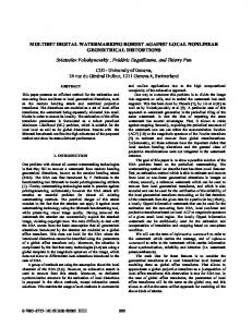
In (30) and (31), Pf and Pm stand for the expressions in the unidimensional case, namely (12) and (13), respectively. The OR function provides poorer performance, but it may be interesting from a security perspective, as we will see in Section 4. Figure 7 shows the resulting ROC’s for different dimensionalities using the AND function; it can be seen that, given one of the probabilities, Pf or Pm , there exists an optimum number of dimensions D∗ which minimizes the other probability. The calculation of D∗ is rather involved, since it depends on the DWR and the DNR, and it will not be accomplished in this paper. Although in our analysis we have assumed the particular form of orthogonality given by (29), the results are essentially the same for any general †

Note that the value of L/D must be large enough to assure the validity of the CLT.

0

0

10

10

−5

D = 40 D = 10

−1

10

10

−10

10

−2

D=1

10

−15

D = 100

10

Pf

Pf

D = 20 D = 50

D=1

−20

−4

10

D=2

10

D = 200

−25

−5

10

10

−30

10

−3

10

−6

−15

10

−10

10

10

−5

10

0

10

−6

10

−5

10

Pm

10

−4

−3

10 P

−2

10

−1

10

0

10

m

(a) DNR = 20 dB

(b) DNR = 10 dB

Figure 7. ROC for AND region and different dimensionalities of the projection subspace, with DWR = 20 dB and L = 1000.

case of orthogonality. Figure 8-a compares the theoretical results with numerical ones by means of Monte Carlo simulations using matrices S whose elements are i.i.d. Gaussian random variables‡ . Orthogonality in the columns of S is desirable to achieve the best performance possible; however, as we will discuss in Section 4, the introduction of a certain correlation between the components of the projected signal may be interesting from a security point of view. The obtention of a specified covariance matrix in the projected domain is very simple: let R be the D × D desired covariance matrix whose eigen-decomposition is R = PΛPT .

(32)

If S is an orthonormal matrix and we use the projection matrix defined as 1

S′ , SΛ 2 PT ,

(33)

2 then it is easy to show that Rrx = E{rx rTx } = σX R, with rx = S′T x. Figure 8-b shows numerical results by means of Monte Carlo simulations for different degrees of correlation between components in 2-D quantization, with stronger correlations yielding poorer performance.

4. SECURITY The concept of security in watermarking is still diffuse, in the sense that there is no full agreement on what are the relevant variables to assess the security of a system. For people working in the field of cryptography it is well known the Kerckhoff’s principle,11 which claims that the security of a cryptographic system must rely solely on the secret key; the translation of this principle to our scenario implies that all parameters of the algorithm (∆, T , L, D and the chosen detection function, in our case) are publicly known, with exception of the projection matrix S, which can be made pseudorandom to play the role of the secret key. This way, the security analysis of this section will deal with attacks (obviously intentional) whose aim is to gain knowledge of the secret matrix S. This approach allows to make a clear distinction between attacks to security and attacks to robustness, which were addressed in Section 3. Another approach to the assessment of watermarking security relying on these concepts can be found in.4 Although a great amount of threats to security exist, much of the researchers’ attention has been paid to the category of oracle attacks, i.e. those attacks which try to exploit the availability of detection devices (usually in ‡

Note that, with i.i.d. Gaussian elements, the columns of S will be almost perfectly orthogonal for moderately high values of L.

0

0

10

10

−1

10

−1

10

−2

Pf

Pf

OR region AND region

10

OR region −2

10

AND region

−3

10

10

uncorrelated components correlated components

−3

−4 −6

10

−5

10

10

−4

−3

10 P

−2

10

−1

10

0

10

10

−3

10

−2

−1

10

10

0

10

Pm

m

(a) S with orthogonal columns

(b) S with non-orthogonal colums

Figure 8. ROC with 2-dimensional quantization, for DWR = DNR = 20 dB, and L = 100. Solid lines and points stand for theoretical and empirical values (with Gaussian random vectors), respectively.

the form of a black box). We will focus on the so-called sensitivity attack ,12 which consists in modifying the signal at the detector input in a component-by-component basis, in order to estimate the points on the boundary of the detection region; when this region is given by a hyperplane, which is the case of SS detection based on linear correlation (4), the attack succeeds when L different points of the boundary are correctly estimated; moreover, this is equivalent to estimating the secret vector v of Equation (1). The complexity of a successful attack for SS-based methods have been shown to be O(L).13 Most of the proposed approaches in the literature5, 7, 8 to overcome this problem rely on the construction of more involved detection regions, much of them parameterized in a non-linearly fashion, which in many cases may yield hard-to-implement schemes. What we propose here is to take advantage of the properties of the generalized QPD scheme described in Section 3.3 to construct detection regions based on the combination of linearly parameterized regions. The advantage of this approach is that the detection region can be progressively complicated just by increasing the dimensionality of the projected subspace, but still allowing the design of implementable schemes from a practical point of view. It its important to note that classical sensitivity attacks performed for spread spectrum will not work well for QPD, since that algorithm is designed assuming that there is only a single boundary to estimate. For example, in the simplest form of QPD, with scalar quantization (D = 1), the detection function strongly resembles that of SS, but the boundary of the detection region in QPD (Figure 3-a) is multiple, since it is defined by shifted versions of the hyperplane orthogonal to the secret vector s. In this section, a new sensitivity attack suited to this new scenario is proposed. The main steps of the algorithm are outlined in the following lines. The proposed algorithm tries to estimate a projection vector in the AND region case or a linear combination of the projection vectors in the OR region case. In fact, in both cases it tries to compute the minimum-normed ˆ = 0. vector which modifies the watermarked vector in such a way that the output of the detector is M The algorithm consists in the addition of an attacking vector α to the watermarked signal y. This α is initially set to an observation of a random variable which is iteratively modified. In the k-th iteration, one of Lβ possible modification vectors β k mod Lβ § , scaled by τk (τ0 is a parameter of the algorithm), is chosen, and added − and subtracted to the attacking vector, yielding γ + k = α + τk β k mod Lβ and γ k = α − τk β k mod Lβ . The two resulting vectors are scaled to be in the boundary of the detection region: + + δ+ k = ak γ k

a+ k

(34) δ+ k)

δ+ k)

with the minimum positive number such that dAN D (y + = 0 or dOR (y + = 0, and equivalently for + − δ− . If min(||δ ||, ||δ ||) < ||α|| (but always in the first iteration), then α = arg min k k k ρ={δ + ,δ − } ||ρ||. k

§

k

In our implementation we have chosen that the modification is component-by-component, but it could also be done by choosing a random vector for the modification.

If α is not modified for any β k mod Lβ , the value of τk is reduced¶ ; otherwise, τk+1 = τk . The value of τ0 − will determine the rate of convergence of the algorithm. The computation of a+ k (or ak ) is performed by a first + − ˆ = 0. After step multiplying the γ k (γ k ) by a constant (2 in the implementation) until the detector output is M that, the boundary is estimated by a bisection algorithm. When successful, the algorithm provides one vector y + α at the boundary of the detection region which is at minimum distance of the watermarked vector y. For the AND region, the vector α is co-linear with one of the columns of S; for the OR region, α is a linear combination of the columns of S. Note that, due to the nature of the algorithm, the addition of a random dither signal in the projected domain will not provide any additional security to the system. To quantitatively assess the security of our system, we must first define some measures: • For the AND region, we define ηAN D (α, S) , max

i=1,...,D



|αT si | ||α|| · ||si ||



,

(35)

where si is the i-th column of the projection matrix S. Notice that (35) can be interpreted as the cosine of the minimum angle formed by α and the columns of S, and gives a measure of the co-linearity between α and the column of S that the algorithm tried to estimate. Similarly, we can define for the OR region   |αT vi | , (36) ηOR (α, S) , max ||α|| · ||vi || i=1,...,2D where vi is one of the 2D possible linear combinations obtained by multiplying the columns of S by ±1. • Let us also define ϕ(α) , 20 log10



||α|| K



,

(37)

where K is the norm of the minimum-normed vector which moves the marked signal outside√of the detection region. Note that, for the AND region, K = T , but for the OR region we have K = DT . Equation (37) is related to the saving in the power necessary to perform a successful attack (i.e. generating an unwatermarked signal) when the output of the algorithm is taken into account. With the definitions given by (35), (36) and (37), we can give two alternative, although related, definitions of security level : 1. the number of iterations N ∗ of the algorithm which are necessary to bring the value of (35) or (36), depending on the considered detection function, above a certain threshold; 2. the number of iterations N ∗ of the algorithm necessary to bring the value of (37) below a certain threshold. Figure 9 shows the results for the AND regions: as can readily be seen, the larger D, the better the estimate for a given number of iterations of the algorithm. This seems to be somewhat contradictory, but bear in mind that the probability of finding a correct projection direction is increasing with D. Anyway, the algorithm succeeds in finding a correct direction regardless the value of D. The results for the OR region are represented in Figure 10. The situation with respect to the AND region is radically different: the estimation becomes more difficult for increasing values of D, and even for a large number of iterations, the estimation is really poor, which can be attributed to the characteristics of the to-be-minimized function (the norm of vector α). At this point, we want to remark that the classical sensitivity attack (i.e., intended for SS) applied to QPD in the simplest case of D = 1 yielded really poor results (ηAN D = ηOR < 0.1). ¶

In our implementation, Lβ = L and τk+1 = 0.7τk .

4

4

2.5

x 10

2.5

x 10

D=1 D=2 D=5 D=10

D=1 D=2 D=5 D=10

2

1.5

1.5

N∗

N∗

2

1

1

0.5

0.5

0

0

5

10

15

20

25

ϕ

30

35

40

45

50

0

0

0.1

0.2

0.3

0.4

0.5

η

0.6

0.7

0.8

0.9

1

(b)

(a)

Figure 9. Security levels for the AND region (L = 1024). 4

4

2.5

x 10

2.5

x 10

D=1 D=2 D=5 D=10

D=1 D=2 D=5 D=10

2

1.5

1.5

N∗

N∗

2

1

1

0.5

0.5

0

0

10

20

30

ϕ

40

50

60

0

0

0.1

0.2

0.3

0.4

(a)

0.5

η

0.6

0.7

0.8

0.9

1

(b)

Figure 10. Security levels for the OR region (L = 1024).

Be aware that the proposed algorithm provides a method to unwatermark watermarked signals, but it is not sufficient to generate valid watermarked signals, because the it is only aimed at disclosing one secret vector or a linear combination of all of them, depending on the detection function. To disclose the whole projection matrix, the algorithm should be modified to search only in the remaining possible directions. For example, considering an AND detection function, if the attacker knows that the projection matrix is orthogonal, once one column is disclosed, the algorithm proposed here can be used to estimate the other ones by restricting the modifying vectors to directions orthogonal with the already disclosed one. Of course, this simple adaptation of the algorithm is not suitable to perform a complete attack when OR functions are considered. Taking into account the previous adaptation, we want to note that the use of non-orthogonal projection matrices can be interesting to improve security.

5. CONCLUSIONS AND FURTHER WORK In this paper, a novel method for detection in quantization-based watermarking has been presented and analyzed. The method is based on the quantization of a projection function applied to the host signal, and it can be adapted

to the requirements of a wide variety of scenarios by an appropriate selection of its parameters, which allow to select the desired levels of robustness and security, but keeping always in mind the existence of a trade-off between these two quantities, in the sense that their simultaneous maximization, although desirable, is not possible. The most remarkable features of this new method are its great improvement in performance compared to traditional spread spectrum methods, and the high security level against oracle-like attacks provided by the the combination of the OR detection function with a moderately high number of dimensions in the projected domain. Although the results presented in this paper are very promising, a lot of work remains to be done. Concerning robustness, the optimization of the number of dimensions of the projected subspace, and the study of the threshold in QPD in terms of the Neyman-Pearson criterion appear as interesting future lines to explore. Finally, concerning the security aspects, we are mainly interested in the refinement of the proposed sensitivity attack for the estimation of the whole projection matrix, so as to provide a more exact security level.

ACKNOWLEDGMENTS This work was partially funded by Xunta de Galicia under projects PGIDT04 TIC322013PR and PGIDT04 PXIC32202PM; MEC project DIPSTICK, reference TEC2004-02551/TCM; FIS project G03/185, and European Comission through the IST Programme under Contract IST-2002-507932 ECRYPT. ECRYPT disclaimer: the information in this document reflects only the authors’ views, is provided as is and no guarantee or warranty is given that the information is fit for any particular purpose. The user thereof uses the information at its sole risk and liability.

REFERENCES 1. T. Liu and P. Moulin, “Error exponents for one-bit watermarking,” in Int. Conf. on Acoustics, Speech and Signal Processing (ICASSP), 3, pp. 65–68, 6-8 April 2003. 2. F. P´erez-Gonz´alez, F. Balado, and J. R. Hern´ andez, “Performance analysis of existing and new methods for data hiding with known-host information in additive channels,” IEEE Transactions on Signal Processing 51, pp. 960–980, April 2003. 3. B. Chen and G. Wornell, “Quantization Index Modulation: a class of provably good methods for digital watermarking and information embedding,” IEEE Transactions on Information Theory 47, pp. 1423–1443, May 2001. 4. F. Cayre, C. Fontaine, and T. Furon, “Watermarking security: theory and practice,” IEEE Transactions on Signal Processing , 2005. To appear. 5. J. J. Eggers, J. K. Su, and B. Girod, “Public key watermarking by eigenvectors of linear transforms,” in European Signal Processing Conference (EUSIPCO), (Tampere, Finland), September 2000. 6. T. Furon and P. Duhamel, “An asymmetric public detection watermarking technique,” in Proc. of the third Int. Workshop on Information Hiding, A. Pfitzmann, ed., pp. 88–100, Springer Verlag, (Dresden, Germany), September 1999. 7. T. Furon, B. Macq, N. Hurley, and G. Silvestre, “JANIS: Just Another n-order Side-Informed Watermarking Scheme,” in International Conference on Image Processing (ICIP), 2, pp. 22–25 September, (Rochester, NY, USA), 6-8 April 2002. 8. M. F. Mansour and A. H. Tewfik, “Secure detection of public watermarks with fractal decision boundaries,” in European Signal Processing Conference (EUSIPCO), (Toulouse, France), 2002. 9. M. Barni and F. Bartolini, Watermarking Systems Engineering, Signal Processing and Communications, Marcel Dekker, 2004. 10. L. P´erez-Freire, F. P´erez-Gonz´alez, and S. Voloshinovskiy, “Revisiting quantization-based data-hiding: exact analysis and results,” IEEE Transactions on Signal Processing , 2004. Submitted. 11. A. Kerckhoff, “La cryptographie militaire,” Journal des sciences militaires 9, pp. 5–38, January 1883. 12. I. J. Cox and J. P. M. G. Linnartz, “Public watermarks and resistance to tampering,” in IEEE International Conference on Image Processing ICIP’97, 3, (Santa Barbara, California, U.S.A.), October 1997. 13. T. Kalker, J. P. Linnartz, and M. van Dijk, “Watermark estimation through detector analysis,” in IEEE Int. Conf. on Image Processing, ICIP’98, pp. 425–429, (Chicago, IL, USA), October 1998.