Detection of a Change-point in Student-t Linear Regression Models

Statistical Papers manuscript

Detection of a Change-point in Student-t Linear Regression Models Felipe Osorio, Manuel Galea1

?

Departamento de Estad´ıstica, Universidad de Valpara´ıso, Chile. Received: June 5, 2003; revised version: June 14, 2004

Abstract In this work the Schwarz Information Criterion (SIC) is used in order to locate a change-point in linear regression models with independent errors distributed according to the Student-t distribution. The methodology is applied to data sets from the financial area. Key words: Change-point, Student-t model, regression model, Schwarz information criterion. 1 Introduction The problem of change-points has been a topic of permanent interest in Statistical literature. Chernoff and Zacks (1964), Gadner (1969), Hawkins (1992), Sen and Srivastava (1975) and Worsley (1979) have studied the problem of change points in the mean of a normal distribution. Horv´ath (1993) and Chen and Gupta (1995) studied the problem of simultaneous change-points in the mean and variance, also of a normal distribution. For a review and many further results along these lines we refer to Cs¨org˝o and Horv´ath (1997). The corresponding problem of change-points in the coefficients of a linear regression model has also been analyzed, under the assumption of normality, by several authors. Quant (1958, 1960) discusses estimates and hypotheses tests for a regression model in two phases. Brown, Durbin and Evans (1975) use recursive residuals to detect change-points in regression models. Hawkins (1989) uses the union-intersection principle and Kim (1994) the likelihood ratio test to detect change-points. Cs¨org˝o and Horv´ath (1997) ? Address: Departamento de Estad´ıstica, Universidad de Valpara´ıso, Casilla 5030, Valpara´ıso, Chile. E-mail: [email protected]

2

Felipe Osorio, Manuel Galea

discuss some asymptotic results about this topic. Recently, Chen (1998) proposes the use of the Schwarz information criterion, SIC, to detect a change-point in linear regression models, also under the assumption of normality. See also Chen and Gupta (2001). Let us consider a sequence of observations, (xT1 , Y1 ), (xT2 , Y2 ), . . . , (xTn , Yn ). The objective of this paper is to test hypothesis of the form: H0 : Yi = xTi β + ²i ,

i = 1, 2, . . . , n,

(1)

i.e, regression coefficients does not change, against H1 : Yi = xTi β 1 + ²i , Yi = xTi β 2 + ²i ,

i = 1, . . . , k, i = k + 1, . . . , n.

(2)

where, β 1 = (β0 , β1 , . . . , βp−1 )T ,

∗ β 2 = (β0∗ , β1∗ , . . . , βp−1 )T ,

that is, a change exists (in the regression coefficients) in an unknown position k, denominated change-point. In this work Chen’s (1998) results are extended to the independent Student-t linear regression model. The use of the t-distribution as an alternative to the normal distribution, has frequently been suggested in literature, for example, Lange, Little and Taylor (1989) propose the t-distribution for robust modeling in linear regression models. Firstly, the methodology described by Chen (1998) is presented. Later on, the procedure of detection of change-points is presented for independent Student-t linear regression models. Finally, this methodology is applied to a group of data from the literature and to data from Chilean stock market. A comparison with the normal model is carried out in both cases. 2 Detection of a change-point in Normal linear regression models Consider the linear regression model Yi = xTi β + ²i ,

i = 1, . . . , n,

where xi , i = 1, . . . , n, corresponds to the i-th line of the design, X matrix n × p, β = (β0 , β1 , . . . , βp−1 )T is the vector of unknown parameters, and ²i indicates a random error. In this section we suppose that the errors ²i are independent random variables, each one with a distribution N (0, σ 2 ), where σ 2 is an unknown parameter (σ 2 > 0). In this way, we have that responses, Yi , i = 1, . . . , n, are independent random variables distributed as N (xTi β, σ 2 ). For the change-point hypothesis (equations (1) and (2)) consider the following notation, where k = p, . . . , n − p, Y 1 = (Y1 , Y2 , . . . , Yk )T ,

Y 2 = (Yk+1 , . . . , Yn )T ,

Detection of a Change-point in Student-t Linear Regression Models



xT1  xT2  X1 =  .  ..



3



 xTk+1  xTk+2    X2 =  .  .  .. 

  , 

xTk

xTn

The work by Chen (1998) proposes transforming the process of hypothesis testing in a procedure of model selection using the Schwarz Information Criterion, (SIC) defined by: b + s log n, SIC = −2 L(θ) b corresponds to the log-likelihood function evaluated on the maxwhere L(θ) imum likelihood estimate of the parameters, s is the number of model parameters and n is the sample size. Note that maximizing the log-likelihood function is equivalent to minimizing the Schwarz information criterion. Under H0 , there is a model that does not present any change in the regression coefficients; on the other hand, under H1 there is a collection of models with change-points at the positions p or p + 1 or . . . or n − p. The objective is, therefore, to select a model from the previous group. The maximum likelihood estimates for θ = (β T , σ 2 )T , under H0 , are given by b = (XT X)−1 XT Y ,

σ b2 =

1 (Y − Xb)T (Y − Xb). n

The Schwarz information criterion under H0 , denoted by SIC(n), is given for: b + (p + 1) log n SIC(n) = −2 L0 (θ) = n log Q(b) + n(log 2π + 1) + (p + 1 − n) log n, b corresponds to the maximum of the log-likelihood function where L0 (θ) under H0 and Q(b) = (Y − Xb)T (Y − Xb). Consider the model under the alternative hypothesis, i.e, that with a change-point at the position k, (k = p, . . . , n − p). In this case, θ = (β T1 , β T2 , σ 2 )T , and the maximum likelihood estimates turn out to be b1 = (XT1 X1 )−1 XT1 Y , b2 = (XT2 X2 )−1 XT2 Y , 1 σ b2 = {(Y 1 − X1 b1 )T (Y 1 − X1 b1 ) + (Y 2 − X2 b2 )T (Y 2 − X2 b2 )}. n then the Schwarz information criterion under H1 , denoted by SIC(k), for k = p, . . . , n − p, is b + (2p + 1) log n SIC(k) = −2 Lk (θ) = n log{Q(b1 ) + Q(b2 )} + n(log 2π + 1) + (2p + 1 − n) log n, b corresponds to the maximum of the log-likelihood function where Lk (θ) under H1 .

4

Felipe Osorio, Manuel Galea

Selection Criteria The selection criteria is to choose a model with a change-point in the k position, if for some k SIC(n) > SIC(k). When the null hypothesis is rejected, the maximum likelihood estimate of the change-point in the regression coefficients, denoted by b k, must satisfy, SIC(b k) = min{SIC(k) : p ≤ k ≤ n − p}, = max{Lk (θ) : p ≤ k ≤ n − p}. 3 Detection of a change-point in independent Student-t linear regression models Consider the independent Student-t linear regression model, where the errors ²1 , ²2 , . . . , ²n are independent and identically random variables with t(0, φ, ν) distribution. Next, the maximum likelihood estimates under both hypotheses are described: one without changes in the regression coefficients (H0 ) and the other with a change in a given position k. The EM algorithm is used to estimate the parameters due to its simple implementation. In the first place the estimates are presented under H0 . In this case the log-likelihood function of θ = (β T , φ)T is L0 (θ) = n log K(ν) −

n n ν+1 X log φ − log{1 + d2i (β, φ)/ν}, 2 2 i=1

where d2i = d2i (β, φ) =

(Yi − xTi β)2 , φ

i = 1, . . . , n,

Γ ( ν+1 2 ) K(ν) = √ πν Γ ( ν2 ) The score functions are given by U (β) =

n 1 1 X vi (Yi − xTi β)xi = XT V(Y − Xβ), φ i=1 φ

U (φ) = −

n n 1 X n 1 vi (Yi − xTi β)2 = − + 2 + 2 QV (β), 2φ 2φ i=1 2φ 2φ

where V = diag(v1 , v2 , . . . , vn ), with vi = vi (θ) =

ν+1 , ν + d2i

i = 1, . . . , n,

QV (β) = (Y − Xβ)T V(Y − Xβ).

Detection of a Change-point in Student-t Linear Regression Models

5

The likelihood equations correspond to a nonlinear system of equations which should be solved via iterative methods. In this work we suppose that the degrees of freedom ν is known. Fern´andez and Steel (1999), alert on the estimate ν and they notice that in this case the function of log-likelihood is unbounded and that indeed it corresponds to an nonregular estimation problem. Due to this, it is suggested (see Lange, Little and Taylor, 1989) to estimate θ = (β T , φ)T considering a set of acceptable values for ν and to choose the one that maximizes the function of log-likelihood. In our case, the Schwarz information criterion will be used to choose among some values of ν. The estimation using the EM algorithm will now be considered. The observed log-likelihood function under the model without changes, turns out to be n 1 1 L0 (Y |v; θ) = − log 2πφ + log |V| − QV (β). 2 2 2φ The EM algorithm maximizes the log-likelihood iteratively through two stages. The (r+1)-th step of the algorithm is summarized as follows: E Step: Starting from initial estimates for θ = (β T , φ)T , weight estimates (r) vi are obtained through the conditional expectations (r)

E(Ui |Yi ; θ (r) ) = vi

=

ν+1 ν+

2(r) di (β (r) , φ(r) )

,

with

(Yi − xTi β (r) )2 , i = 1, 2, . . . , n. φ(r) and where the independent random variables, Ui ∼ Gamma((ν + 1)/2, (ν + d2i )/2). 2 (r)

di

=

M Step: Using the weights obtained at the E step of the algorithm, the maximum likelihood estimates are obtained, β (r+1) = (XT V(r) X)−1 XT V(r) Y , with

(r)

φ(r+1) =

1 Q (r) (β (r) ), n V

(r)

V(r) = diag(v1 , v2 , . . . , vn(r) )

and the algorithm proceeds between E and M step until the sequence θ (r) converge. Under a change model on the regression coefficients in a given k position, it is possible to show that the log-likelihood function turns out to be k

Lk (θ) = n log K(ν) − −

n ν+1X log φ − log{1 + d2i (β 1 , φ)/ν} 2 2 i=1

n ν+1 X log{1 + d2i (β 2 , φ)/ν}, 2 i=k+1

6

Felipe Osorio, Manuel Galea

where θ = (β T1 , β T2 , φ)T and the associated score functions are given by: U (β 1 ) =

1 T X V1 (Y 1 − X1 β 1 ), φ 1 U (φ) = −

U (β 2 ) =

1 T X V2 (Y 2 − X2 β 2 ), φ 2

n 1 + {QV1 (β1 ) + QV2 (β2 )}, 2φ 2φ2

with V1 = diag(v1 , v2 , . . . , vk ),

V2 = diag(vk+1 , . . . , vn ).

To develop the estimate procedure using the EM algorithm, the observed log-likelihood function under the model with a change in a k position (given) takes the form: n n 1 1 log 2π − log φ + log |V1 | − QV1 (β 1 ) 2 2 2 2φ 1 1 + log |V2 | − QV2 (β 2 ) 2 2φ

Lk (Y |v; θ) = −

The (r +1)-th iteration of the algorithm of expectation maximize consists in two steps, described as follows: (r)

E Step: The conditional expectations vi given by (r)

E(Ui |Yi ; θ (r) ) = vi

=

should be obtained, this are ν+1

ν + d2i (θ (r) )

,

which are based on the following weights function,  (r) (Yi − xTi β 1 )2    , i = 1, 2, . . . , k, φ(r) d2i (θ (r) ) = (r) T 2    (Yi − xi β 2 ) , i = k + 1, . . . , n. (r) φ where the independent random variables Ui follow a Gamma distribution with parameters (ν + 1)/2 and (ν + d2i )/2. M Step: Using the estimates obtained at the E step, likelihood estimates are calculated by: (r)

(r)

(r)

(r)

(r+1)

= (XT1 V1 X1 )−1 XT1 V1 Y 1 ,

(r+1)

= (XT2 V2 X2 )−1 XT2 V2 Y 2 , o 1n (r) (r) = QV(r) (β 1 ) + QV(r) (β 2 ) . 1 2 n

β1 β2

φ(r+1) with (r)

(r)

(r)

(r)

V1 = diag(v1 , v2 , . . . , vk ),

(r)

(r)

V2 = diag(vk+1 , . . . , vn(r) ).

Detection of a Change-point in Student-t Linear Regression Models

7

The implementation of the EM algorithm under H1 , requires a slight modification of the iteratively reweighted least square, because the scale parameter φ remains fixed along the sequence of observations. Now the Schwarz information criterion is presented under the model without changes in the regression coefficients and under the model with a change in the k given position. Under H0 , we have that b + (p + 1) log n SIC(n) = −2 L0 (θ) = −2 n log K(ν) + n log φb + (p + 1) log n +(ν + 1)

n X

(3)

b φ)/ν} b log{1 + d2i (β,

i=1

and under H1 (for given k), the Schwarz information criterion is given by b + (2p + 1) log n SIC(k) = −2 Lk (θ) = −2 n log K(ν) + n log φb + (2p + 1) log n

(4)

k n hX i X 2 b b , φ)/ν} b b +(ν + 1) log{1 + d2i (β + log{1 + d ( β , φ)/ν} . 1 2 i i=1

i=k+1

Note that when ν → ∞ the expressions corresponding to the normal case (Chen, 1998) are obtained. Selection Criteria Using the Schwarz information criterion (equations (3) and (4)) the hypothesis of no change on the regression coefficients H0 is rejected if: SIC(n) > min{SIC(k) : p ≤ k ≤ n − p}. Or equivalently if, 4n < 0, where 4n = min{SIC(k) − SIC(n) : p ≤ k ≤ n − p}. If H1 is accepted, i.e, there is a change-point at the regression coefficients, then the change position is estimated via maximum likelihood, in a way that b k has to satisfy. SIC(b k) = min{SIC(k) : p ≤ k ≤ n − p}. To make conclusions about change-points statistically significant, the level of significance α and its associated critical value cα (cα ≥ 0) are introduced. So instead of rejecting H0 when 4n < 0, the hipothesis of no change on the regression coefficients is rejected if 4n + cα < 0

(5)

8

Felipe Osorio, Manuel Galea

where cα satisfies the relationship: 1 − α = P [4n + cα < 0 |H0 ] = P [Zn < p log n + cα |H0 ] b b where Zn = max{−2(L0 (θ)−L k (θ)) : p ≤ k ≤ n−p} and using the theorem 1.3.1 in Cs¨org˝o and Horv´ath (1997), we have that cα ≈

1 a2 (log n)

{dp (log n) − log log[1 − α + exp(−2edp (log n) )]−1/2 }2 − p log n (6)

with a(x) = (2 log x)1/2 ,

dp (x) = 2 log x +

³p´ p log log x − log Γ 2 2

Therefore we propose to use (6) to calculate approximate cα values, for a level of significance α. If it is suspected that a change-point exists in the k position, when carrying out the test of change by means of Zn , there are n − 2p tests being done out, one for each k. A useful technique for finding approximates critical values is based on the inequality of Bonferroni. Using this method one has the following criteria, to reject H0 at a nominal α level if Zn > χ21−α/(n−2p) (p). For the normal case, LRT has an exact distribution, in which case, H0 is rejected if Zn > F1−α/(n−2p) (p, n − 2p).

Some Considerations It is evident that implementing a routine for change-points detection by means of the SIC procedure is quite simple; it is also possible to observe that the methodology of detection for changes in the regression coefficients considered here is equivalent to the procedure for testing a change-point using the Likelihood ratio test given in Cs¨org˝o and Horv´ath (1997). However, they notice that the region of rejection of the hypothesis is conservative and indeed large samples should be used in (6) to test H0 against H1 . The methodology for detection of change-points delineated here corresponds to a test of a unique change. Chen and Gupta (1997) mention a method proposed by Vostrikova (1981) who outlines a procedure of binary segmentation, in which the problem of detection of multiple changes is subdivided in to equivalent simple detection processes. The estimation of parameters for the problem of detection of changes, in the regression coefficients and the approach of model selection conforms the base of an S-Plus routine, created for developing these calculations.

Detection of a Change-point in Student-t Linear Regression Models

9

4 Applications In this section, the methodology derived in this work is applied to data frequently analyzed in the literature (see Chen (1998) and Chang and Huang (1997)). Data of returns from a share belonging the Chilean stock market is also considered. 4.1 Holbert’s data (Chen, 1998)

BSE

50

100

150

200

250

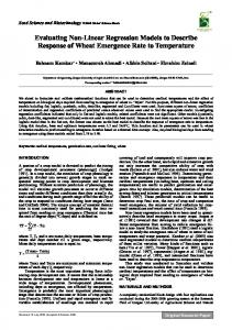
Holbert (1982) use a simple linear regression model with changes in the coefficients from a Bayesian point of view. Later on, Chen (1998) analyzed this data using the SIC method to detect changes in the mean for Normal linear regression models. In this section, Holbert data will be used to illustrate the SIC procedure, for the detection of change-points in independent Student-t linear regression models. Sales volume (in millions) of the Boston stock market (BSE) is considered as a response variable and the sales volume of the New York stock market (NYAMSE) as a regressive variable. The data corresponds to the period between January 1967 and November 1969. Figure 1 shows the scatter plot of Holbert’s data.

10000

12000

14000 NYAMSE

Fig. 1 Holbert’s data scatter plot

16000

18000

10

Felipe Osorio, Manuel Galea

The SIC procedure was applied for the detection of changes, for the Student-t linear regression model with a set of values for the degrees of freedom, as well as for the normal model. The summary of results is in the following table. Table 1 Results of SIC Procedure t Model ν=1 ν=4 ν=8 ν = 30 ν→∞

SIC(n) 363.358 358.082 359.332 360.855 361.453

min SIC(k) 357.416 355.035 356.669 358.074 358.475

b k 9 23 23 23 23

A possible change-point is detected in the period b k = 23, and this result is in concordance with the conclusion obtained by Chen (1998). Using the Schwarz Information Criterion, the Student-t model with ν = 4 was chosen to develop some later analysis. The parameter estimates for the model with a change-point in position 23 is presented. The results for the normal model are also presented. There is an appreciable difference on the coefficients estimates for the Student-t model with ν = 4 degrees of freedom and the normal model; in particular, the difference among the intercepts of both models is evident. However, the scatter plot with fitted regression lines for the model with a change-point in position 23, do not reveal a remarkable difference between the normal model and the Student-t model with ν = 4 (see Table 2 and Figure 2). Table 2 Estimates for the model with a change in the 23rd position. t Model ν=4 ν→∞

Cases 1 24 1 24

to to to to

23 35 23 35

Estimate β0 β1 -96.0781 0.0162 15.2759 0.0065 -110.5475 0.0178 11.0747 0.0067

In accordance with the above-mentioned, the condition (5) was verified, obtaining that detected changes do not turn out to be significant. The analysis by means of the Bonferroni method reveals that the Student-t model for Holbert’s data does not detect changes in the coefficients. Note however, that the sample size for these data is small, so that this decision can be conservative.

Detection of a Change-point in Student-t Linear Regression Models

200 BSE

150 50

100

150 50

100

BSE

200

250

ν→∞

250

ν=4

11

10000

12000

14000

16000

18000

10000

12000

14000

NYAMSE

16000

18000

NYAMSE

Fig. 2 Scatter plots and adjust regression

Observations in 4, (- - -) correspond to previous periods to observation 24 (from where a change was detected in the sequence). Notice that, in spite of perceiving a graphic difference in the fitted regression lines, these changes are not significant. ν→∞

364

SIC

362

360 356

360

358

SIC

362

366

364

368

ν=4

23 0

5

10

15

20

23 25

index

30

0

5

10

15

20

25

30

index

Fig. 3 Diagram SIC(k) vs. k

The graph of the Schwarz information criterion against the index has been suggested, i.e, SIC(k) vs. k, because it is possible to obtain the maximum likelihood estimate of k from this graph. In both diagrams the 23rd position may be as a possible maximum likelihood estimate for the changepoint. Note, however, that for the normal model, the SIC(k) values are bigger than these for the Student-t model with ν = 4 and, therefore, it is suggested to use this last one as an alternative to the normal distribution. In Osorio (2001) the vulnerability of the normal model to atypical observations is shown, indeed, some diagrams of local influence are considered indicating that for the t with ν = 4 this influence is smaller.

12

Felipe Osorio, Manuel Galea ν=4

ν→∞ 35

2

2

35 34

0

1

34

-1

0

1

ordered data values

33

-1

ordered data values

33

-2

-1

0

1

2

-2

quantiles of standard normal

-1

0

1

2

quantiles of standard normal

Fig. 4 Quantile plots

From the quantile plots a slight deviation of the supposed distributional is appreciated for the t with ν = 4 as for the Normal model (ν → ∞), therefore, the quantile plots do not offer conclusive information in this respect.

4.2 Detection of a change in the systematic risk The Capital Asset Pricing Model (CAPM) establishes that the expected return on an asset is equal to the risk free rate return plus a prize for risk. This model was independently derived by Sharpe (1964), Lintner (1965), and Mossin (1966). Let r be a random variable, which denotes the asset return. According to the CAPM, the expected value of r, is given by: E(r) = rf + β(E(rm ) − rf ),

(7)

where rf is the risk free rate return, rm corresponds to the market return and β denotes the systematic risk of the asset. An extension of the model (7) given by E(r) − rf = α + β(E(rm ) − rf ), (8) incorporates a coefficient α that denotes the asset return independent to the market fluctuations. It is usual to consider a linear regression model to estimate α and β, this is, given a group of n observations for the return of the asset, the market return and the risk free return, one has rt − rf t = α + β(rmt − rf t ) + ²t ,

t = 1, . . . , n,

(9)

where rt denotes the return of the asset in the period t, rmt is the market return in the period t, t = 1, . . . , n. Here we suppose that ²1 , ²2 , . . . , ²n are independent random errors such that ²t ∼ t(0, φ, ν), t = 1, . . . , n. The main interest in the CAPM model is to carry out inferences regarding the systematic risk β. To estimate the beta parameter from (9), the least squares method is frequently used. Also to carry out inferences regarding

Detection of a Change-point in Student-t Linear Regression Models

13

0.4 0.2 -0.2

0.0

Concha y Toro

0.6

0.8

1.0

the parameters, we generally suppose that the returns follow a normal distribution. It is important to note that the estimate of the systematic risk on Latin American markets (emergent) has some peculiarities, such as atypical observations and points leverages. In this respect there are robust estimates for β (see Duarte and Mendes (1997)); however, changes in the systematic risk have not been considered. The CAPM was used to data corresponding to monthly returns, adjusted by equity variations, of “Vineyards Concha y Toro”. IPSA, was used as the return for the market and as risk free rate was used the interest rate in the sale of discounted bonds of the Central Bank (PDBC) based monthly. The data corresponds to the period among the months of March 1990 to April 1999. Figure 5 shows the scatter plot for the data asset Vineyards Concha y Toro.

-0.3

-0.2

-0.1

0.0

0.1

0.2

IPSA

Fig. 5 Vineyard Concha y Toro data scatter plot

The procedure of detection of a point of change was developed considering a independent t linear regression model for a set of values for freedom degrees using SIC procedure. The results are as follows: Table 3 Results of SIC Procedure. t Model ν=1 ν=4 ν=8 ν = 30 ν→∞

SIC(n) -172.304 -172.136 -159.518 -135.362 -116.382

min SIC(k) -175.924 -173.098 -157.776 -135.803 -123.829

ˆ k 100 100 (100) 25 25

14

Felipe Osorio, Manuel Galea

Note that the possible periods detected as change-points for the normal model and for the t model, with ν = 1 or 4, are different; also, for the t model with 8 degrees of freedom a change is not detected (the position among parenthesis corresponds to min SIC(k)). However, the SIC for the Student-t model with ν = 1 or 4 are smaller than for the normal model. Using the minimum information approach, the t model was chosen with 1 degree of freedom. In what follows this model will be used to carry out later analysis. The estimate of parameters was developed for the model with a change in position k, obtaining the following, Table 4 Estimate for the model with a change in position k. t Model

Cases

ν=1

Estimates α β -0.0069 0.3021 -0.0111 1.1096 0.0372 1.5995 -0.0019 0.4799

1 to 100 101 to 110 1 to 25 26 to 110

ν→∞

As a result of some interest, to verify that for the normal distribution the change detected in position 25 is significant to 5%, on the other hand for the t-distribution with any one of the considered degrees of freedom, the changes are not significant, and therefore for these data, the Student-t model does not detect any change in the regression coefficients. This decision is ratified when carrying out the procedure of Bonferroni. Indeed, a change is only detected in the coefficients when it is considered the normal model.

0.8 0.6 0.4 -0.2

0.0

0.2

Concha y Toro

0.4 0.2 -0.2

0.0

Concha y Toro

0.6

0.8

1.0

ν→∞

1.0

ν=1

-0.3

-0.2

-0.1

0.0

0.1

0.2

-0.3

-0.2

-0.1

IPSA

0.0

0.1

0.2

IPSA

Fig. 6 Dispersion and straight line of Regression Diagram

The observations in 4, ( - - - ) correspond to the previous periods to the point where a change happens in the sequence. Although for the normal model a point of change is detected in the regression coefficients, as for the

Detection of a Change-point in Student-t Linear Regression Models

15

t model this change is not significant. Consider the results of the estimate parameters for the model without changes that is presented in the following table: Table 5 Estimate for the model without changes in the coefficients. t Model ν=1 ν→∞

log-likelihood 93.2026 65.2417

α b -0.0084 0.0129

βb 0.3462 0.8884

Starting from this, the use the Student-t model with ν = 1 is suggested, to estimate the systematic risk through the estimates for β in the model that does not present any change. The diagram was also carried out βb(i) vs. i (see Figure 7), where βb(i) denotes the maximum likelihood estimator of β without the i-th observation. Here certain stability is noticed by the βb(i) , so that it is clear that the t model reduces the influence of atypical observations.

0.7 0.6 beta(i)

0.5 0.3

0.4

0.5 0.3

0.4

beta(i)

0.6

0.7

0.8

ν→∞

0.8

ν=1

0

20

40

60

80 index

100

120

140

0

20

40

60

80

100

120

140

index

Fig. 7 βb(i) vs. i plot

The diagram was also obtained βb{k} vs. k where k indicates the number of observations included for the calculation of the estimate of β. In spite of the natural fluctuations of this estimates when having few observations, note that this graph reveals the position of change detected by the normal model. However, a greater stability for the Student-t model with ν = 1, is appreciated, by this we perceive a certain insensibility of the Student-t model in the face of changes in the coefficients in this case.

16

Felipe Osorio, Manuel Galea

2

ν→∞

2

ν=1

1 0

beta(k)

-1

0 -1

beta(k)

1

25

0

20

40

60

80

100

0

20

40

k

60

80

100

k

Fig. 8 Diagram βb{k} vs. k

Also notice that the Student-t model with ν = 1 has values SIC(k) smaller than of the Normal model. Starting from the approach of minimum information the use of the Student-t distribution is suggested with ν = 1 instead of the normal distribution for this data set. ν→∞

-176

-174

-120

-115

SIC

-170 -172

SIC

-168

-166

-110

-164

ν=1

100 0

20

40

60

80

index

100

25 0

20

40

60

80

100

index

Fig. 9 SIC(k) Diagram vs. k

In Osorio (2001) there are remarks on the great impact that the period of February 28 1991 (observation 12) has on the MLE for the normal model, on the contrary of the t model with ν = 1 where the influence of the periods is smaller. Also, one can observe an evident deviation from the supposed distributional for the normal model (see Figure 10). Therefore, the abovementioned suggests the use of distribution t with ν = 1. Consider tables 4 and 5, note that when using the t model with ν = 1 the appreciation that one has of the systematic risk is different from that of the normal model. Indeed, when using the estimates of parameters obtained by means of the t with ν = 1 (model does not present changes in the coefficients), the asset of Vineyards Concha y Toro is less risky than

Detection of a Change-point in Student-t Linear Regression Models

17

for the normal model. This information can be particularly useful for risk administrators or of stocks portfolios. ν=1

ν→∞

4

4

110

2

ordered data values

108

0

2 0

ordered data values

109

1

2

3 -2

-1

0

quantiles of standard normal

1

2

-2

-1

0

1

2

quantiles of standard normal

Fig. 10 Quantile Plots

Conclusion It is evident that the detection of points of change through the SIC offers an important simplification, allowing a simple computer implementation. It was also indicated that the approach of testing hypothesis proposed in this work is equivalent to the likelihood ratio test for locate change points, therefore an expression was presented for the calculation of approximate quantile values and this way testing hypothesis with a significant level. It is of interest to notice that this expression is valid for any distribution of the errors so that the decision can be conservative for small sample sizes.

Acknowledgements The authors acknowledge the partial financial support from Project Fondecyt 1000424-Chile. The authors are grateful to the referees whose comments and suggestions were valuable to improve the exposition of the paper.

References 1. Chan Y. P. and Huang, W. T. (1997). Inferences for the linear errors-invariables with changepoint models. Journal of the American Statistical Association 92, 171-178. 2. Chen, J. (1998). Testing for a change point in linear regression models. Communications in Statistics - Theory & Methods 27, 2481-2493.

18

Felipe Osorio, Manuel Galea

3. Chen, J. and Gupta, A. K. (1995). Likelihood procedure for testing change points hypothesis for multivariate gaussian model. Random Operators and Stochastic Equations 3, 235-244. 4. Chen, J. and Gupta, A. K. (1997). Testing and locating variance change point with application to stock prices. Journal of the American Statistical Association 92, 739-747. 5. Chen, J. and Gupta, A. K. (2001). On change point detection and estimation. Communications in Statistics - Simulation & Computation 30, 665-697. 6. Cs¨ org˝ o, M. and Horv´ ath, L. (1997). Limit Theorems in Change-Point Analysis. Wiley, New York. 7. Duarte, A. M. and Mendes, B. V. M. (1998). Robust estimation of systematic risk in emerging stock markets. Emerging Markets Quaterly 1, 85-95. 8. Fern´ andez, C. and Steel, M. (1999). Multivariate student t regression models: pitfalls and inference. Biometrika 86, 153-167. 9. Horv´ ath, L. (1993). The maximum likelihood method for testing changes in the parameters of normal observations. Annals of Statistics 21, 671-680. 10. Lange, K. L.; Little, J. A. and Taylor, M. G. (1989). Robust statistical modeling using the t distribution. Journal of the American Statistical Association 84, 881-896. 11. McLachlan, G. L. and Krishnan, T. (1997). The EM Algorithm and Extensions. Wiley, New York. 12. McQuarrie, A. D. R. and Tsai, C. L. (1998). Regression and Time Series Model Selection. World Scientific Publishing, Singapore. 13. Osorio, F. (2001). Detecci´ on de un punto de cambio en modelos de regresi´ on lineal t independiente, Tesis para optar al t´ıtulo de ingeniero en Estad´ıstica. Departamento de Estad´ıstica. Universidad de Valpara´ıso, Chile.