ground maps, and update a motion image that keeps the motion statistics. ..... ios ranged from lunch rooms to underground train stations. Half of these ...
MITSUBISHI ELECTRIC RESEARCH LABORATORIES http://www.merl.com
Detection of Temporarily Static Regions by Processing Video at Different Frame Rates
Fatih Porikli
TR2007-040
October 2007
Abstract This paper presents an abandoned item and illegally parked vehicle detection method for single static camera video surveillance applications. By processing the input video at different frame rates, two backgrounds are constructed; one for short-term and another for long-term. Each of these backgrounds is defined as a mixture of Gaussian models, which are adapted using online Bayesian update. Two binary foreground maps are estimated by comparing the current frame with the backgrounds, and motion statics are aggregated in a likelihood image by applying a set of heuristics to the foreground maps. Likelihood image is then used to differentiate between the pixels that belong to moving objects, temporarily static regions and scene background. Depending on the application, the temporary static regions indicate abandoned items, illegally parked vehicles, objects removed from the scene, etc. The presented pixel-wise method does not require object tracking, thus its performance is not upper-bounded to error prone detection and correspondence tasks that usually fail for crowded scenes. It accurately segments objects even if they are fully occluded. It can also be effectively implemented on a parallel processing architecture. AVSS 2007
This work may not be copied or reproduced in whole or in part for any commercial purpose. Permission to copy in whole or in part without payment of fee is granted for nonprofit educational and research purposes provided that all such whole or partial copies include the following: a notice that such copying is by permission of Mitsubishi Electric Research Laboratories, Inc.; an acknowledgment of the authors and individual contributions to the work; and all applicable portions of the copyright notice. Copying, reproduction, or republishing for any other purpose shall require a license with payment of fee to Mitsubishi Electric Research Laboratories, Inc. All rights reserved. c Mitsubishi Electric Research Laboratories, Inc., 2007 Copyright 201 Broadway, Cambridge, Massachusetts 02139
MERLCoverPageSide2
Detection of Temporarily Static Regions by Processing Video at Different Frame Rates Fatih Porikli Mitsubishi Electric Research Laboratories (MERL), Cambridge, USA
Abstract This paper presents an abandoned item and illegally parked vehicle detection method for single static camera video surveillance applications. By processing the input video at different frame rates, two backgrounds are constructed; one for short-term and another for long-term. Each of these backgrounds is defined as a mixture of Gaussian models, which are adapted using online Bayesian update. Two binary foreground maps are estimated by comparing the current frame with the backgrounds, and motion statistics are aggregated in a likelihood image by applying a set of heuristics to the foreground maps. Likelihood image is then used to differentiate between the pixels that belong to moving objects, temporarily static regions and scene background. Depending on the application, the temporary static regions indicate abandoned items, illegally parked vehicles, objects removed from the scene, etc. The presented pixel-wise method does not require object tracking, thus its performance is not upper-bounded to error prone detection and correspondence tasks that usually fail for crowded scenes. It accurately segments objects even if they are fully occluded. It can also be effectively implemented on a parallel processing architecture.
1. Introduction Significant amount of effort has been devoted to tracking based abandoned item detection [1, 2, 3, 4, 5] in video surveillance. Most of these methods are designed for a multiple, overlapping field-of-view camera system that is calibrated onto a ground plane. They assume the scene is not crowded, occlusions are minimal, and moving objects can be accurately initialized using only motion information. Besides, they require solving a harder problem of object tracking and object detection as an intermediate step. There have been similar work [6, 7] for single camera setups. In [7] a gradient-based method is applied to the static foreground regions to detect the type of the static regions by analyzing the change in the amount of edge energy
associated with the boundaries of the static foreground region between the current frame and the background image. The static region is an abandoned (removed) object if there are significantly more (less) edges. This algorithm requires precise boundaries and fails in case of cluttered multimodal scenes. A common solution to handle multimodal backgrounds and compensate for illumination variances is to use mixture models. In [8] an expectation maximization (EM) based online adaptation method to learn the mixture of Gaussians is proposed. A fixed number of models are updated at each pixel using a set of constant learning parameters. Online EM update causes a weak model to be dissolved into a dominant one in case the weak and dominant models have similar mean values and the variance of the weak model is much larger than the dominant model. To solve this problem, Porikli and Tuzel [9] presented an online Bayesian update mechanism. This method is shown to generate accurate models while enabling assignment of different number of models at every pixel depending on the local intensity distributions. There exists a class of problems that traditional single foreground/background detection methods still cannot solve. For instance, objects left behind in public places, such as suitcases, packages, etc. do not fall into either of the two categories. They are static; therefore, they should be labeled as background. On the other hand, they should not be ignored as they do not belong to the original scene background. Here, we present a method that use multiple backgrounds and does not require object tracking. The main motivation is that the recently changed pixels that stay static after they changed can be distinguished from the actual background pixels and the pixels corresponding to the moving regions by analyzing the intensity variance in different temporal scales. We employ the mixture of Gaussian models and update them online using a Bayesian update mechanism. We compute long-term and short-term foreground maps from these background models. We compare the foreground maps, and update a motion image that keeps the motion statistics. These statistics are then used to differentiate between the pixels that belong to the moving objects,
Motion Motion Image Image
Foreground Foreground Long Long
Foreground Long
Hypothesis
Change
Moving object
Change
No Change
Candidate abandoned object
No Change
Change
Uncovered background
No Change
Scene background
Foreground Foreground Short Short
Image
Foreground Short
I
Input frames
time
Figure 1. Long-term and short-term backgrounds are learned by processing video at different frame rates.
the temporarily static image areas, and the perpetually static parts of the background scene. Depending on the application, the temporary static areas (of the recently changed pixels) indicate abandoned items, illegally parked vehicles, objects removed from the scene, etc. The background models have identical initial parameters, thus, they require minimal fine tuning in the setup stage. Our method can also be effectively implemented on a parallel processing architecture.
2. Two Backgrounds To detect an abandoned item (or an illegally parked vehicle) we need to know how it alters the temporal and spatial statistics of the video data. We built our method on the observation that an abandoned item was not a part of the original scene, it was brought into the scene not that long ago, and it stayed still after it was left. In other words, it can be considered as a temporarily static object which was not there before. This means that by learning the prolonged scene background and the moving foreground regions, we can hypothesize whether a pixel corresponds to an abandoned item or not. The prolonged background can be determined by maintaining a statistical background model that captures the most consistent modes of the color distribution of each pixel in extended durations of time. From this prolonged background, the foreground pixels that do not fit into the statistical models are obtained. Depending on the adaptation rate of the prolonged background, the regions corresponding to the temporary static objects, e.g. abandoned items, can be mistaken as a part of the background (faster adaptation rates) or grouped with the moving regions (slower adaptation rates). A single prolonged background is insufficient to separate the temporarily static pixels from the prolonged static pixels. As opposed to the single background approaches, we use two backgrounds to learn both the prolonged (longterm) background BL and the temporarily static (shortterm) background BS . It is possible to improve the temporal granularity by employing multiple backgrounds at different
Figure 2. Hypotheses on the long- and short-term foregrounds.
temporal scales. Using the short-term background, we determine the short-term foreground pixels that correspond to the moving objects in the scene. The pixels of the objects ceased moving are rapidly blended into the short-term background. Each of the backgrounds is defined as a mixture of Gaussians models. We formulate each pixel as layers of 3D multivariate Gaussians. Each layer corresponds to a different appearance of the pixel. We perform our operations on the RGB color space. We apply a Bayesian update mechanism. At each update, at most one layer is updated with the current observation. This assures the minimum overlap over layers. We also determine how many layers are necessary for each pixel and use only those layers during the foreground segmentation phase. This is performed with an embedded confidence score. Both of these backgrounds have identical initial parameters; the initial mean and variance of the marginal posterior distribution, the number of the prior measurements, the degrees of freedom, and the scale matrix, etc. Construction of the backgrounds is illustrated in Figure 1. The short-term background is updated at a higher frequency than the long-term background. At a higher frequency, the short-term background learns the underlying distribution faster, thus, the changes are blended rapidly. In contrast, the long-term background is more resistant against the temporary changes. At every frame, we estimate the long- and short-term foregrounds by comparing the current frame I by the background models BL and BS . We obtain two binary foreground maps FL and FS where F (x, y) = 1 indicates the pixel (x, y) is changed. The long-term foreground FL shows the variations in the scene that were not there before including the moving objects, temporarily static objects, moving shadows, noise, and illumination changes that the background models fail to adapt. The short-term foreground FS contains the moving objects, noise, etc. However, it does not show the temporarily static regions that we want to detect. Depending on the foreground mask values, we formulate
original
FL
FS
L
result
Figure 3. First row: t = 350. Second row: t = 630. The long-term foreground FL captures moving objects and temporarily static regions. The short-term foreground FS captures only moving objects. The likelihood L gets greater as the object stays longer.
the following hypotheses as shown in Figure 2: 1. FL (x, y) = 1 ∧ FS (x, y) = 1; (x, y) is a pixel that may correspond to a moving object since I(x, y) does not fit any backgrounds. 2. FL (x, y) = 1 ∧ FS (x, y) = 0; (x, y) is a pixel that may correspond to an abandoned item. 3. FL (x, y) = 0 ∧ FS (x, y) = 1; (x, y) is a scene background pixel that was occluded before. 4. FL (x, y) = 0 ∧ FS (x, y) = 0; (x, y) is a scene background pixel since its value I(x, y) fits both backgrounds BL and BS . The short-term background adapts itself to the relatively consistent changes, but it does not learn temporary color changes due to motion of the objects. Thus, such a pixel is marked as FS (x, y) = 1 in the short-term foreground. Since the long-term background is updated less frequently, a temporary change cannot alter the long-term background. The pixel is also marked as FL (x, y) = 1 in the long-term foreground mask. In case a pixel that was a part of the scene background is occluded for sometime and then uncovered, the long-term foreground will still be zero, FL (x, y) = 0. The long-term background is updated less frequently hence it is not responsive enough to adapt to the new color during the occlusion. Yet, the short-term background is responsive and adapts itself during the occlusion, which causes FS (x, y) = 1. A stationary pixel will be blended into the short-term background i.e. FS (x, y) = 0 if it stays stationary long enough. Assuming this duration is not prolonged to blend the pixel in the scene background. As a result, the long-term foreground will be one, FL (x, y) = 1. This is expected for the left behind items.
If no change is observed in any backgrounds, i.e. FL (x, y) = 0 and FS (x, y) = 0, the pixel is considered as a part of the static scene. This case requires the pixel to have the same color distribution for prolonged periods of time. Sample foreground maps showing some of these cases is given in Figure 3. We aggregate the frame-wise motion statistics into a likelihood image L(x, y) by updating the pixel-wise values at each frame as L(x, y) + 1 FL (x, y) = 1 ∧ FS (x, y) = 0 L(x, y) − k FL (x, y) 6= 1 ∨ FS (x, y) 6= 0 L(x, y) = maxe L(x, y) > maxe 0 L(x, y) < 0 where maxe and k are positive numbers. The likelihood image enables removing noise in the detection process. It also controls the minimum time required to assign a static pixel as an abandoned item. For each pixel, the likelihood image collects the evidence of being an abandoned item. Whenever this evidence elevates up to a preset level, i.e. L(x, y) > maxe , we mark the pixel as an abandoned item pixel and raise an alarm flag. The evidence threshold maxe is defined in term of the number of frames and it can be chosen depending on the desired responsiveness and noise characteristics of the system. In case the foreground detection process produces noisy results, higher values of maxe should be preferred. High values of maxe decrease the false alarm rate. On the other hand, higher the preset level gets longer the minimum duration a pixel takes to be classified as a part of an abandoned item. The decay parameter k governs how fast the likelihood should decrease if no evidence is provided. It also determines the responsiveness of the system in case the abandoned item is removed, in which case the pixels returns their original background values before the detection, or blended into the scene background. To set the alarm flag off imme-
diately after the removal of abandoned object, the value of decay constant should have a large value. The decay parameter can be set proportional to the evidence threshold. This means only a single parameter is needed for the likelihood image. Neither of the backgrounds and their mixture models depends on the likelihood image preset values. This makes the detection robust against the variations of the evidence and decay parameters that can be set comfortably without struggling to fine tune the overall system.
3. Foreground Detection Our background model [9] is most similar to adaptive mixture models [8] but instead of mixture of Gaussian distributions, we define each pixel as layers of 3D multivariate Gaussians. Each layer corresponds to a different appearance of the pixel. We perform our operations in the RGB color space. Using Bayesian update, we are not estimating the mean and variance of the layer, but the probability distributions of mean and variance. We can extract statistical information regarding to these parameters from the distribution functions. We use the expectations of mean and variance for change detection, and variance of the mean for confidence. Bayesian update algorithm maintains the multimodailty of the background model. Learned background statistics is used to detect the changed regions of the scene. We determine how many layers are necessary for each pixel and use only those layers during foreground segmentation phase. The number of layers required to represent a pixel is not known beforehand so background is initialized with more layers than needed. Usually we select three to five layers. In more dynamic scenes more layers are required. Using the confidence scores we determine how many layers are significant for each pixel. As we observe new samples for each pixel we update the parameters for our background model. At each update, at most one layer is updated with the current observation. This assures the minimum overlap over layers. We order the layers according to confidence score and select the layers having confidence value greater than the layer threshold. We refer to these layers as confident layers. We start the update mechanism from the most confident layer. If the observed sample is inside the 2.5σ of the layer mean, which corresponds to 99% confidence interval of the current model, parameters of the model are updated. Lower confidence models are not updated. Details can be found in [9].
4. Experimental Results To test the proposed method, we used several public datasets from PETS 2006 [10], i-LIDS [11], and Advanced Technology Center, Amagasaki. The total number of tested
Correctly detected event
Ground truth event
AB-easy
frame no
1400 AB-medium
2300
4250
4800
False alarm
1330 1500
2200
4500
2770
4800
AB-hard
1400
2570
4800 4850
5200
PV-medium
400
690
2320
3270
Figure 4. Detected events for i-LIDS dataset.
sequences were 32. The data included different resolutions, 180×144, 320×240, 640×480, and 720×576. The scenarios ranged from lunch rooms to underground train stations. Half of these sequences depict scenes that are not crowded. Other sequences have more complex scenarios with multiple people sitting, standing, walking, etc. There are sequences that have parked vehicles. In all sequences people walk at variable speeds. The abandoned items are left for varying durations; from 10 seconds to 2 minutes. Most sequences contain small (10 × 10) abandoned items. Some sequences have multiple abandoned items. We grouped the similar sequences into the same set and reported the result for several sets. The sets AB-Easy, ABMedium, and AB-Hard, which are included in i-LIDS Challenge, are recorded in an underground train station. Set PETS is a large closed space platform with restaurants. Sets ATC-1 and ATC-2 are recorded from a wide angle camera of a cafeteria. Sets ATC-3 and ATC-4 are different cameras from a lunch room. Set ATC-5 is a waiting lounge. Since the proposed method is a pixel-wise scheme, it is not difficult to set detection areas in the initialization time. We manually marked the platform in AB-easy, AB-medium, and AB-hard sets, the waiting area in PETS 2006 set, and the illegal parking spots in PV-easy, PV-medium, and PV-hard sets. For the ATC sets, all of the image area is used as the detection area. For the i-LIDS sets, we replaced the beginning parts of the video sequences with 4 frames of the empty platform. For all results, we updated the short-term background at 30 fps, and the long-term background at 1 fps. Our tests show that the processing rates can be set to even much lower values as long as both short and long term rates are proportionally scaled i.e. the short-term rate to 1 fps and the longterm rate to 2 frame-per-minutes (30 times slower). We set the evidence threshold maxe 50 500 depending on the desired responsiveness time. We used k = 1 as the decay parameter. Figure 4 shows the detection results for the i-LIDS
datasets. We reported the performance scores of all sets in Table 1. Tall is the total number of frames in a set and Tevent is the duration of the event in terms of the number of frames on Table 1. We measure the duration right after an item is being left behind. However, it is also possible to measure the duration after the person moved away or after some preset waiting time. Events indicates the number of left behind objects (for PV-medium, the number of the illegally parked vehicles). TD means the correctly detected objects. A detection is considered to be both spatially and temporally continuous. In other words, there might be multiple detections for a frame if the objects are spatially disconnected. FA shows the falsely detected objects. Ttrue and Tf alse is the duration of the correct and false detections. Tmiss is the duration that a left behind item could not be detected. Since we start an event as soon as an object is left, this score does not consider any waiting time. This means that we overestimate our miss rate. As our results show, we successfully detected all abandoned items while achieving a very low false alarm rate. Our method performed satisfactory when the initial frame showed the actual static background. The detection areas have not included any people at the initialization time in the ATC sets, thus the proposed method accurately learned the uncontaminated backgrounds. This is also true for the PV and AB-easy sets. However, the AB-medium and AB-hard sets contained several people, some of who were sitting, in the first frames. This resulted in false detections when those people moved away. Since the background models eventually learns the statistically dominant color values, such false alarms should not occur in the long run due to the fact that the background will be more visible than the people. In other words, the ratio of the false alarms should decrease in time. We do not learn the color distribution of the abandoned items items (or parked vehicles), thus, the proposed method can detect them even if they are occluded. As long as the occluding object, which may be a person who moves between the abandoned item and the camera, has different color than the long-term background, the long-term foreground will show the abandoned item. Representative detection results are given in Figures 56. As visible, none of the moving objects, moving shadows, people that are stationary in shorter durations was falsely detected. Besides, there are no ghost false detections due the inaccurate blending of the abandoned items in the long-term background. Thanks to the Bayesian update, the changing illumination conditions as in PV-medium are properly adapted in the backgrounds. Another advantage of this method is that the alarm is immediately set of as soon as the abandoned item is removed from its previous position. Although we does not know whether the person who left the object is moved away from the object or not, we consider this property as a su-
periority over the tracking based approaches that require a decision net of heuristic rules and context depended priors to detect such event. One shortcoming is that it cannot discriminate the different types of objects, e.g. a person who is stationary for a long time can be detected as a left behind item. This can be, however, an indication of a suspicious behavior as it is not common. To determine object types and reduce the false alarm rate, object classifiers, i.e. a human or a vehicle detector, can be used. Since such classifiers are only for verification purposes, their computation time is negligible.
5. Conclusions We present a computationally efficient and robust method to detect abandoned items and illegally parked vehicles. This method uses two backgrounds that are learned by processing the input video at different frame rates. This method does not depend on tracking. Therefore, it is not restricted to predefined event heuristics that require detection, tracking and identification of every single object in the scene. Unlike the motion vector analysis based approaches, it accurately detects the boundary of abandoned items even if they are occluded. Since it employs pixel-wise operations, it can be implemented for parallel processors.
References [1] E. Auvinet, E. Grossmann, C. Rougier, M. Dahmane, and J. Meunier, “Left-luggage detection using homographies and simple heuristics,” in PETS, 2006, pp. 51–58. [2] J. M. del Rincn, J. E. Herrero-Jaraba, J. R. Gmez, and C. OrriteUruuela, “Automatic left luggage detection and tracking using multicamera ukf,” in PETS, 2006, pp. 59–66. [3] P. T. N. Krahnstoever, T. Sebastian, A. Perera, and R. Collins, “Multiview detection and tracking of travelers and luggage in mass transit environments,” in PETS, 2006, pp. 67–74. [4] K. Smith, P. Quelhas, and D. Gatica-Perez, “Detecting abandoned luggage items in a public space,” in PETS, 2006, pp. 75–82. [5] S. Guler and M. K. Farrow, “Abandoned object detection in crowded places,” in PETS, 2006, pp. 99–106. [6] C. Sacchi, C. Regazzoni, “A distributed surveillance system for detection of abandonedobjects in unmanned railway environments,” in IEEE Transactions on Vehicular Technology, vol. 49, 2000. [7] J. Connell, A. Senior, A. Hampapur, Y. Tian, L. Brown, and S. Pankanti, “Detection and tracking in the IBM PeopleVision system,” Proc. IEEE ICME, 2004. [8] C. Stauffer and E. Grimson, “Adaptive background mixture models for real-time tracking,” in Proc. IEEE Conf. on Computer Vision and Pattern Recognition, Fort Collins, CO, vol. II, 1999, pp. 246–252. [9] F. Porikli and O. Tuzel, “Bayesian background modeling for foreground detection,” in Proc. of ACM Visual Surveillance and Sensor Network, 2005. [10] PETS 2006 Benchmark Data, http://www.cvg.rdg.ac.uk/PETS2006/ data.html. [11] i-LIDS Dataset for AVSS 2007, ftp://motinas.elec.qmul.ac.uk/pub/ iLids.
Table 1. Detection Results
Sets AB-easy AB-med. AB-hard PV-med. PETS ATC-1 ATC-2 ATC-3 ATC-4 ATC-5
Tall 4850 4800 5200 3270 3000 6600 13500 5700 3700 9500
Tevent 2850 3000 3400 1920 1200 3400 6500 2400 2000 5350
Events 1 1 1 1 1 6 18 5 6 11
TD 1 1 1 1 1 6 18 5 6 10
FA 0 1 1 0 0 0 0 0 1 2
Ttrue 2220 1730 2230 1630 950 2350 4740 1390 1300 3160
Tmiss 630 1270 1170 290 250 1100 1850 1010 700 2150
Tf alse 0 970 350 20 10 50 40 0 350 420
1
500
750
1250
1500
2000
2300
2350
2500
3000
Figure 5. Test sequence PV-medium from AVSS 2007 (Courtesy of i-LIDS). A challenge in this video is the rapidly changing illumination conditions that cause dark shadows.
1
1170
1750
2350
3000
3600
4130
4230
4300
4800
Figure 6. Test sequence AB-easy from AVSS 2007 (Courtesy of i-LIDS). The alarm sets of immediately when the item is removed even though the luggage was stationary 2000 frames (180 × 144).