underwater acoustic communication using orthogonal frequency division multiplex ...... Case 1: No Doppler shift compensation by setting ϵ = 0. ⢠Case 2: Ideal ...
IEEE JOURNAL ON SELECTED AREAS IN COMMUNICATIONS, VOL. 26, NO. 9, DECEMBER 2008
1
Detection, Synchronization, and Doppler Scale Estimation with Multicarrier Waveforms in Underwater Acoustic Communication Sean F. Mason, Christian R. Berger, Student Member, IEEE, Shengli Zhou, Member, IEEE, and Peter Willett, Fellow, IEEE
Abstract—In this paper, we propose a novel method for detection, synchronization and Doppler scale estimation for underwater acoustic communication using orthogonal frequency division multiplex (OFDM) waveforms. This new method involves transmitting two identical OFDM symbols together with a cyclic prefix, while the receiver uses a bank of parallel self-correlators. Each correlator is matched to a different Doppler scaling factor with respect to the waveform dilation or compression. We characterize the receiver operating characteristic in terms of probability of false alarm and probability of detection. We also analyze the impact of Doppler scale estimation accuracy on the data transmission performance. These analytical results provide guidelines for the selection of the detection threshold and Doppler scale resolution. In addition to computer-based simulations, we have tested the proposed method with real data from an experiment at Buzzards Bay, MA, Dec. 15, 2006. Using only one preamble, the proposed method achieves similar performance on the Doppler scale estimation and the bit error rate as an existing method that uses two linearly-frequencymodulated (LFM) waveforms, one as a preamble and the other as a postamble, around each data burst transmission. Compared with the LFM based method, the proposed method works with a constant detection threshold independent of the noise level and is suited to handle the presence of dense multipath channels. More importantly, the proposed approach does not need to buffer the whole data packet before data demodulation, which facilitates future development of online realtime receiver for multicarrier underwater acoustic communications. Index Terms—Underwater acoustic communication, OFDM, wideband channel, detection, synchronization and Doppler scale estimation.
I. I NTRODUCTION
V
ARIOUS data transmission schemes are being actively pursued for underwater acoustic (UWA) communications, including multicarrier modulation in the form of orthogonal frequency division multiplexing (OFDM) [1]–[4], single carrier transmission with time-domain sparse-channel equalization [5] or frequency-domain equalization [6], and multi-input multi-output (MIMO) techniques combined with single carrier [7], [8] or multicarrier [9] transmissions. These
Manuscript received February 29, 2008, revised July 13, 2008. This work is supported by the ONR YIP grant N00014-07-1-0805, the NSF grant ECS 0725562, the NSF grant CNS 0721834, and the ONR grant N0001407-1-0055. This work was partially presented at the IEEE/MTS OCEANS conference, Kobe, Japan, April 2008. The authors are with the Department of Electrical and Computer Engineering, University of Connecticut, 371 Fairfield Way U-2157, Storrs, Connecticut 06269, USA (email: {seanm, crberger, shengli, willett}@engr.uconn.edu). Digital Object Identifier 10.1109/JSAC.2008.0812xx.
transmission schemes are often examined via offline data processing based on recorded experimental data. Towards the development of an online underwater acoustic receiver, detection and synchronization are important, yet often overlooked tasks. Typically, synchronization entails a known preamble, which is easily detected by the receiver, being transmitted prior to the data. Existing preambles used in underwater telemetry are almost exclusively based on linearly frequency modulated (LFM) signals, also known as Chirp signals [10]. This is due to the fact that LFM signals have a desirable ambiguity function in both time and frequency, which matches well to the underwater channel, which is characterized by its large Doppler spread. However, the receiver algorithms are usually matchedfilter based, which try to synchronize a known template to the signal coming from one strong path, while suppressing other interfering paths. This approach suffers from the following two deficiencies: first, the noise level at the receiver has to be constantly estimated to achieve a constant false alarm rate (CFAR), usually accomplished using order statistics; second, its performance will degrade in the presence of dense and unknown multipath channels. Due to the slow propagation speed of acoustic waves, the compression or dilation effect on the time domain waveform needs to be considered explicitly. Once a Doppler scale estimate is obtained, a resampling procedure is usually applied before data demodulation [11]. One method to estimate the Doppler scale is to use an LFM preamble and an LFM postamble around each data burst [11], so that the receiver can estimate the change of the waveform duration. This method estimates the average Doppler scale for the whole data burst. As such it requires the whole data burst to be buffered before data demodulation, which prevents online real-time receiver processing. In this paper, we propose the use of multicarrier waveforms as preamble for underwater acoustic communications. A preamble that consists of two identical OFDM symbols preceded by a cyclic prefix (CP) is used. This training pattern has been studied extensively in wireless OFDM systems for radio channels, see e.g., [12], [13], and has been included as part of the training preamble in the IEEE 802.11a/g standards [14]. The receiver effectively correlates the received signal with a delayed version of itself, since, thanks to the CP structure, the repetition pattern persists even in the presence of
c 2008 IEEE 0733-8716/08/$25.00 �
2
IEEE JOURNAL ON SELECTED AREAS IN COMMUNICATIONS, VOL. 26, NO. 9, DECEMBER 2008
unknown multipath channels [12]. However, the synchronization algorithms that work in wireless radio channels will not perform well in dynamic underwater acoustic channels due to the large waveform expansion or compression, which changes the repetition period to some unknown value. We combine techniques used in underwater telemetry with the elegant, non-parametric self-correlator approach used in radio channels to perform detection, synchronization and Doppler scale estimation based on multicarrier waveforms. We use a bank of parallel branches, with each branch using a selfcorrelator matched to a different repetition period. Detection of a data transmission burst is declared when any of the branches leads to a correlation metric larger than a threshold value. The branch with the largest metric also yields the Doppler scale estimate and coarse synchronization point. We characterize the receiver operating characteristic (ROC) by developing an analytical expression for the probability of false alarm and a Gaussian approximation for the probability of detection. We also analyze the impact of Doppler scale estimation accuracy on the data demodulation performance. These analytical results provide guidelines for selecting the detection threshold and Doppler scale resolution. Compared with the LFM-preamble based approach, the proposed method has the following advantages: (1) the detection threshold is between 0 and 1, and doesn’t depend on the channel or operating SNR; (2) it has a very good detection performance, which is based on the signal energy from all paths rather than only a single path; (3) it leads to accurate Doppler scale estimation; (4) after coarse timing and resampling, it allows the use of fine timing algorithms developed for radio channels, such as [15], [16]; (5) it has a low-complexity implementation when the self-correlation metric is computed recursively [17]. In addition to computer-based simulations, we have tested the proposed method with real data from an experiment at Buzzards Bay, MA, Dec. 15, 2006. Using only one preamble, the proposed method achieves similar performance on the Doppler scale estimation accuracy and the bit error rate as those methods presented in [4], which are based on the LFM preamble and postamble. However, the proposed method needs neither a postamble nor to buffer the whole data burst before demodulation. This facilitates future development of an online realtime receiver for multicarrier underwater acoustic communications. Note that the proposed method provides a point estimate of the Doppler scale at the beginning of a data burst. Therefore, the proposed method is best suited for application scenarios where the Doppler scale stays constant or varies slowly during the data burst duration. When the Doppler scale changes fast, the point estimates need to be frequently updated, e.g., by shortening of the data burst, or, through the use of a tracking algorithm based on point estimates available via inserting multiple synchronization blocks into a long data burst at regular intervals. The rest of this paper is as follows. The system model is described in Section II, and the proposed receiver algorithm is presented in Section III. Detection performance is determined in Section IV, and analysis of the impact of Doppler scale mismatch on the data demodulation performance is investigated in Section V. Section VI contains numerical results,
preamble CP
x
data transmission guard zeros
x
ZP OFDM
ZP OFDM
Fig. 1. A preamble, consisting of two identical OFDM symbols and a cyclic prefix (CP), precedes the data transmission which uses zero padding.
both from simulation and from real data. Section VII contains the conclusion. II. S YSTEM M ODEL To avoid power consumption in the guard interval between OFDM symbols, zero-padded (ZP) OFDM is preferred for data transmission [3], [4]. For synchronization purposes, the preamble consists of two identical OFDM symbols together with a cyclic prefix. The overall transmission structure is shown in Fig. 1. The OFDM parameters can be selected independently for the preamble and the data transmissions. Suppose that K0 subcarriers have been used in the preamble, and one OFDM symbol is of duration T0 . The subcarrier spacing is then 1/T0 and the bandwidth is B = K0 /T0 . Let fc denote the carrier frequency, and fk = fc + k/T0 denote the frequency for the kth subcarrier in passband, where k ∈ S = {−K0 /2, . . . , K0 /2 − 1}. Let Tcp denote the length of the CP, and define a rectangular window of length Tcp +2T0 as � 1 t ∈ [−Tcp, 2T0 ], q(t) = (1) 0 otherwise. The preamble in baseband can be written as � k x(t) = s[k]ej2π T0 t q(t)
(2)
k∈S
and the corresponding passband signal is � � � k j2π t x ˜(t) = Re ej2πfc t s[k]e T0 q(t) � = Re
k∈S
�
s[k]e
j2πfk t
� q(t) ,
(3)
k∈S
where s[k] is the transmitted symbol on the kth subcarrier. The channel impulse response for a time-varying multipath underwater acoustic channel can be described by � c(τ, t) = Ap (t)δ (τ − τp (t)) , (4) p
where Ap (t) is the path amplitude and τp (t) is the timevarying path delay. As in [4], we adopt the following assumptions for algorithm development1. A1) All paths have a similar Doppler scaling factor a such that τp (t) ≈ τp − at. (5) 1 In short, our algorithms are developed based on assumptions A1) and A2). Hence, the application of the proposed method shall be limited to underwater environments where A1) and A2) hold true approximately. Methods suited for application scenarios where different paths have quite different Doppler scales warrant further investigation.
MASON et al.: DETECTION, SYNCHRONIZATION, AND DOPPLER SCALE ESTIMATION WITH MULTICARRIER WAVEFORMS
In general, different paths could have different Doppler scaling factors, e.g., see field test results in [18], [19]. The method proposed in this paper is based on the assumption that all the paths have approximately the same Doppler scaling factor. When this is not the case, part of useful signals are treated as additive noise, which could increase the overall noise variance considerably [4]. However, we find that as long as the dominant Doppler shift is caused by the direct transmitter/receiver motion, as it is the case in our experiment, this assumption seems to be justified. The value of a is usually less than 0.01 when the relative speed between the transmitter and the receiver is below 10 m/s. A2) The path delays τp , the gains Ap , and the Doppler scaling factor a are constant over the preamble duration 2T0 + Tcp . The preamble duration is usually around 50 ms to 200 ms. Assumption A2) is reasonable within such a duration, as the channel coherence time is usually on the order of seconds. When the passband signal in (3) goes through the channel described in (4) and (5), we receive: � � y˜(t) = Re s[k]ej2πfk (1+a)t k∈S
×
�
� � Ap q (1 + a)t − τp e−j2πfk τp
� +n ˜ (t),
(6)
p
where n ˜ (t) is the additive noise. Define τmax = maxp τp , which is usually less than the CP length Tcp . Using the definition of q(t) in (1), we obtain � � � j2πfk (1+a)t y˜(t) = Re Hk s[k]e +n ˜ (t), k∈S
�
t ∈ Tcyclic
� Tcp − τmax 2T0 , = − , (7) 1+a 1+a
where we define the channel transfer function � Ap e−j2πf τp C(f ) =
(8)
p
and the frequency response on the kth subcarrier as Hk = C(fk ).
(9)
Converting the passband
signal y˜(t) to baseband, such that y˜(t) = Re y(t)ej2πfc t , we have: “ ” � j2π Tk +afk t 0 y(t) = Hk s[k]e + n(t) k∈S
= ej2πafc t
�
k
Hk s[k]ej2π T0 (1+a)t + n(t),
(10)
k∈S
for t ∈ Tcyclic and n(t) is the noise at baseband. As expected for CP-OFDM, we observe a cyclic convolution between the signal and the channel in the specified interval, where each subcarrier is only multiplied by the corresponding frequency response. Due to the wideband nature of the underwater channel, the frequency of each subcarrier at baseband has been shifted differently by an amount of afk = afc + ak/T0 .
3
parallel self-correlators
conversion to baseband
window length N1
|x|
window length Nl
|x|
window length NL
|x|
max(x)
≥ Γth
Fig. 2. To account for the time compression/dilation, multiple parallel branches are used, each tuned to a certain period Nl .
III. T HE P ROPOSED A LGORITHM The transmitter sends a baseband waveform embedding a repetition pattern as x(t) = x(t + T0 ),
−Tcp ≤ t ≤ T0 .
(11)
Such a repetition pattern persists in the received signal y(t) even after time-varying multipath propagation as � a T0 −j2π 1+a fc T0 y(t) = e y t+ , 1+a T0 Tcp − τmax ≤t≤ , (12) − 1+a 1+a as can be verified from (10). However, the receiver knows neither the period nor the waveform due to the unknown multipath channel. The problem is then to detect a pattern like (12) from the incoming signal, and infer the repetition period to find the Doppler scale. Although the problem of estimating an unknown delay (synchronization) and Doppler scale has been studied in the literature, [20]–[22], these approaches assume a non-dispersive channel and are therefore based on matched filter processing and the ambiguity function. Ref. [23] has treated random echos, but the suggested approach relies on estimating the unknown channel transfer function jointly with delay and Doppler scale, therefore leading to high-complexity receiver processing, which is not suited for continuous data monitoring and detection. Our proposed approach is to use a bank of self-correlators, see Fig 2, with each one matched to a different periodicity. Detection, synchronization, and Doppler scale estimation are accomplished based on the correlation metrics from the bank of self-correlators. We now present the proposed receiver processing, based on the sampled baseband signal. The baseband signal is usually oversampled at a multiple of the system bandwidth ts = 1/(λB): (13) y[n] = y(t)|t=nts , where the oversampling factor λ is an integer. The receiver processing includes the following steps: 1) Each of the L branches calculates a correlation metric with one candidate value of the window size Nl . The window size Nl shall be close to λK0 , which is the number of samples of one OFDM symbol when no
4
IEEE JOURNAL ON SELECTED AREAS IN COMMUNICATIONS, VOL. 26, NO. 9, DECEMBER 2008
Doppler scaling occurs. For each delay d, the correlation metric corresponding to the window size Nl is M (Nl , d) =
d+Nl −1 ∗ y [i] y[i + Nl ] i=d � , (14) d+Nl −1 2 d+Nl −1 2 |y[i]| · |y[i + N ]| l i=d i=d for l = 1, . . . L. 2) A detection is declared if the correlation metric of any branch exceeds a preset threshold Γth : H1
if:
max |M (Nl , d)| > Γth l
(15)
Since the norm of the metric in (14) is between 0 and 1, the threshold Γth takes a value from [0,1]. 3) The branch with the largest correlation metric is viewed as having the best match on the repetition length. Since Doppler scaling changes the period T0 to T0 /(1 + a), the Doppler scale factor can be estimated as a ˆ=
ˆ λK0 − N , ˆ N
ˆ = arg max |M (Nl , d)| where N {Nl }
(16)
The speed estimate follows as vˆ = cˆ a,
(17)
where c is the speed of sound in water. Additional processing can be used to refine the Doppler scale estimate, as will be shown later on in Section VI. 4) Synchronization is performed on the branch that yields the maximum correlation metric. After the maximum is determined, the start of transmission can be selected as suggested in [12]; starting from the peak the 80% “shoulders” are found (first sample of this correlator branch before and after the peak that is less than 80% of the peak) and the middle is chosen as synchronization point. This is beneficial, since due to the CP structure the correlation metric has a plateau around the peak [12]. Remark 1 (Doppler scale resolution): Since the window size Nl is an integer, the minimum step size on the Doppler scale is 1/(λK0 ). To improve the Doppler scale resolution, the receiver operates on the oversampled baseband signal. The oversampling factor depends on the needed Doppler scale resolution and the parameter K0 . The maximum value of λ is the ratio of the passband sampling rate to the baseband signal bandwidth, which is typically less than 50 in underwater applications. Remark 2 (implementation complexity): The three sliding summations in (14) can be computed recursively. For examd+Nl −1 ∗ y [l]y[i + Nl ]. Instead of ple, define ψ(Nl , d) = i=d summing over Nl multiplications, one can use ψ(Nl , d+1) = ψ(Nl , d)+y ∗ [d+Nl ]y[d+2Nl ]−y ∗ [d]y[d+Nl ], (18) which amounts to two complex multiplications and two complex additions for each update. Hence, for each delay d, the metric M (Nl , d) in (14) can be computed by no more than seven complex multiplications, six complex additions, one square root operation, and one division. Note that the
complexity does not depend on the window size. Such a lowcomplexity approach was implemented in a DSP board for one self-correlator branch [17]. Remark 3 (fine-timing): With the estimated Doppler scale a ˆ, the receiver can resample the preamble. This way, the “wideband” channel effect of frequency-dependent Doppler shifts can be reduced to the “narrowband” channel effect of frequency-independent Doppler shifts [4]. The fine-timing algorithms developed for narrowband radio channels, such as those in [15], [16] can be applied on the resampled preamble. This way, the “first” path can be synchronized [16], instead of the “strongest” path in case of the LFM based method. Due to channel fading, the strongest path can appear at random positions within the delay spread, which is undesirable for the task of data block partitioning after the synchronization. In contrast, the position of the first path is more stable. So far, we have described the general procedure of the proposed detection, synchronization, and Doppler scale estimation algorithm, while some parameters are left to be specified. Important questions include: • How to set the detection threshold? • How many parallel branches are needed? What is the desired Doppler scale resolution? We next address these questions by analyzing the detection performance in Section IV, and the data demodulation performance under Doppler scale mismatch in Section V. IV. R ECEIVER O PERATING C HARACTERISTICS The output of each correlator is a random variable due to the additive noise. The probabilities of false alarm Pf a and detection Pd are the probabilities of the correlator output exceeding a threshold Γth under the “no signal” and “signal” hypotheses, respectively. We now analyze the false alarm and detection probabilities of a single branch, as a function of the threshold Γth and the Doppler scale a. This will give us an understanding of the necessary Doppler scale spacing in the parallel self-correlator structure for detection purposes. Due to over-sampling, the summations in the metric given in (14) of the lth branch can be well approximated with continuous time integrals: � t+Tˆ � � y(τ )∗ y(τ + Tˆ ) dτ t ˆ , M T,t = � �2 � t+Tˆ � t+Tˆ �� � 2 ˆ |y(τ )| dτ · dτ + T ) �y(τ � t t (19) where T0 , t = d · ts . (20) Tˆ = Nl · ts = 1+a ˆ A. Probability of False Alarm When no signal is present, y(t) = n(t). Since B Tˆ ≈ K0 , 0 −1 we can find a set of orthonormal basis functions {fi (t)}K i=0 , such that K 0 −1 � nt,i fi (τ ), τ ∈ [t, t + Tˆ] (21) n(τ ) = n(τ + Tˆ) =
i=0 K� 0 −1
nt+Tˆ,i fi (τ ),
i=0
τ ∈ [t, t + Tˆ].
(22)
MASON et al.: DETECTION, SYNCHRONIZATION, AND DOPPLER SCALE ESTIMATION WITH MULTICARRIER WAVEFORMS
Assume that n(t) is a Gaussian noise process, then nt,i and nt+Tˆ,i are independent and identically distributed Gaussian random variables. Define2 nt = [nt,0 , . . . , nt,K0 −1 ]T and nt+Tˆ = [nt+Tˆ,0 , . . . , nt+Tˆ,K0 −1 ]T , and their normalized ˜ t = nt /�nt � and n ˜ t+Tˆ = nt+Tˆ /�nt+Tˆ �. The versions n correlator output (19) can be simplified to the inner product between two unit length vectors as � � ˜H ˜ t+Tˆ . M Tˆ, t = n (23) t n Finding the probability of false alarm can now be linked to the Grassmannian line packing problem in [24]. Specifically, ˜ t can be viewed as coordinates of a point on the surface n of a hypersphere with unit radius, centered around the origin. This point dictates a straight line in a complex space C K0 that ˜ t and passes through the origin. The two lines generated by n ˜ t+Tˆ have a distance defined as: n � (24) ˜ t+Tˆ |2 , ˜ t+Tˆ ) := sin(θt ) = 1 − |˜ d(˜ nt , n nH t n where θt denotes the angle between these two lines. The ˜ t+Tˆ ) is known as “chordal distance” [24]. distance d(˜ nt , n ˜ t and n ˜ t+Tˆ Since n(t) is additive white and Gaussian, n are uniformly distributed on the surface of the hypersphere. ˜ t+Tˆ is Without loss of generality, we can assume that n ˜ t is uniformly distributed, to evaluate the fixed a priori and n distribution of the chordal distance. Based on [25, eq. (34)] (which was derived based on the geometrical framework in [26]), we infer
˜ t+Tˆ ) < z = z K0 −1 , 0 < z < 1. nt , n (25) Pr d2 (˜ Hence, the probability of false alarm is
Pf a = Pr |M (Tˆ, t)| > Γth � � ˜ t+Tˆ ) < 1 − Γ2th = Pr d2 (˜ nt , n = (1 − Γ2th )K0 −1 .
(26a) (26b) (26c)
Note that Pf a does not depend on the power of the additive noise. Once the threshold Γth is chosen, a constant false alarm rate (CFAR) is achieved independent of the noise level. B. Probability of Detection Assume that the signal is present, we rewrite (10) as y(t) = xc (t) + n(t), where the signal is � j2π k (1+a)t xc (t) = ej2πafc t Hk s[k]e T0 ,
(27)
integration is done in a proper window where xc (t) is well defined as in (28), we can easily obtain: �� � t+Tˆ ∗ ˆ E y(τ ) y(τ + T ) dτ = Tˆφxx (Tˆ, Tˆ), t
� � Tcp − τmax T0 (1 + 2ˆ a − a) , t ∈ Tplateau := − 1+a (1 + a)(1 + a ˆ) �� E
t+Tˆ
� |y(τ )|2 dτ
k∈S
Treating the signal as deterministic unknown, we define the autocorrelation function of xc (t) as � 1 t+T xc (τ )xc (τ + ΔT )dτ. (29) φxx (T, ΔT ) = T t The noise is viewed as wide sense stationary, and we define its autocorrelation function as φnn (τ ). Assuming that the 2 Bold upper case and lower case letters denote matrices and column vectors, respectively; (·)T , (·)∗ , and (·)H denote transpose, conjugate, and Hermitian transpose, respectively. | · | and � · � stand for for the absolute value of a complex number and the norm of a vector, respectively.
��
t+Tˆ
=E
t
(30)
� |y(τ + Tˆ )|2 dτ
t
= Tˆ [φxx (Tˆ, 0) + φnn (0)],
t ∈ Tplateau . (31)
In [12], the absolute value of the correlation metric has been approximated as a Gaussian random variable to derive some approximate results. We would like to follow the same principle here. To this end, we propose to approximate the mean of the correlator output as: � �� �� � Tˆ |φxx (Tˆ, Tˆ )| � � E �M Tˆ, t � ≈ ˆ T φxx (Tˆ, 0) + Tˆφnn (0) αγ , t ∈ Tplateau , = (32) γ+1 where γ = φxx (Tˆ, 0)/φnn (0) is the signal-to-noise-ratio (SNR) at the receiver, and α is the correlation coefficient |φxx (Tˆ, Tˆ )| . (33) α= φxx (Tˆ, 0) The variance can be approximated as � �� 2γ 3 + 5γ 2 + 3γ + 1 �� � � � Var �M Tˆ, t � ≈ , t ∈ Tplateau . 2K0 (γ + 1)4 (34) The variance in (34) was derived in the radio channel case without Doppler scaling where |α| = 1. We argue that it can still be used in the case with Doppler scaling, since the variation of the correlation output is mainly due to additive noise. We now specify the correlation coefficient α. Based on (28), we have for t ∈ Tplateau � ˆ � 1 t+T � ∗ ˆ ˆ xc (τ )xc (τ + Tˆ ) dτ φxx (T , T ) = (35a) Tˆ t � � ˆ = e−j2πafc T Hk s[k]Hl∗ s∗ [l] ×
t ∈ Tcyclic . (28)
5
1 Tˆ
�
k∈S l∈S h
t+Tˆ
e
j2π(1+a)
k T0
τ − Tl (τ +Tˆ ) 0
i
dτ,
(35b)
t
which lead to
��� � |φxx (Tˆ, Tˆ )| = � Hk s[k]Hl∗ s∗ [l]e−j2π(1+�)l � � × ejπ(1+�)(k−l) sinc [(1 + )(k − l)] �, (36) k∈S l∈S
where sinc(x) = sin(πx)/(πx) and (1 + ) = (1 + a)/(1 + ˆa) ˆ. Assume with a ˆ = T0 /Tˆ − 1 from (20). Therefore, ≈ a − a that is tiny, we approximate sinc[(1 + )(k − l)] ≈ δ[k − l]. For constant amplitude modulation |s[i]|2 = σs2 , we have � � �� � 2� 2 −j2πk(a−ˆ a) � ˆ ˆ |Hk | e |φxx (T , T )| ≈ σs � (37) �. k∈S
6
IEEE JOURNAL ON SELECTED AREAS IN COMMUNICATIONS, VOL. 26, NO. 9, DECEMBER 2008
1
1 approx.: μ approx.: μ ±2σ sim.: μ sim: μ ±2σ noise: μ noise: μ +2σ
0.9 0.8 0.7
γ = 10 dB
0.8 0.7
0.5 0.4
0.5 0.4
0.3
0.3
γ = 0 dB
0.2
γ = 0 dB
0.2
0.1 0
γ = 10 dB
0.6 |M(ε)|
|M(ε)|
0.6
approx.: μ approx.: μ ±2σ sim.: μ sim: μ ±2σ noise: μ noise: μ +2σ
0.9
0.1 0
0.5
1 1.5 2 2.5 c⋅ε: speed mismatch in m/s
3
3.5
(a) non-dispersive
0
0
0.5
1 1.5 2 2.5 c⋅ε: speed mismatch in m/s
3
3.5
(b) dispersive
Fig. 3. Statistics of the correlator output, including the mean μ and standard deviation σ as a function of the unknown speed for two different levels of SNR γ; (a) non-dispersive channel with a single path, (b) dispersive channel with an exponential decay profile.
Similar approximation can be done for φxx (Tˆ, 0). We thus have � � 2 −j2πk(a−ˆ a) � � k∈S |Hk | e
α≈ . (38) 2 k∈S |Hk | In summary, with α approximated in (38), the mean μα approximated in (32), and the variance σα approximated in (34), an approximate expression for the probability of detection in Tplateau is � �� � �� � Γth − μα � � ˆ Pd = Pr �M T , t � ≥ Γth ≈ Q , (39) σα √ �∞ 2 where Q(x) = (1/ 2π) x e−t /2 dt. C. Numerical Validation To confirm the theoretical analysis, we use numerical simulation using the following steps: 1) Generate the baseband signal via (10) and sample it as in (13). 2) Compare the statistics of the correlator output at signal start t = 0 on a branch with Nl = λK0 . For the non-dispersive channel with a single path, the mean of the correlator (32) can be simplified to �� � ��� γ αγ � � = |sinc [K(a − a ˆ)]| . (40) E �M Tˆ, 0 � = γ+1 γ +1 The simulation results for the non-dispersive channel are shown in Fig. 3(a); we observe that the loss of correlation due to the unknown speed is modelled well by the sinc function, while the approximation of the standard deviation is fairly exact for the low SNR case but only of the right magnitude for the high SNR case. For dispersive channels we average over different channel realizations, where we choose an exponentially decaying channel profile that loses about 20 dB within 10 ms. For each channel realization, we evaluate the mean and variance of the
Gaussian approximation, then average these by approximating them via a single Gaussian distribution with matched moments. Since this is basically a Gaussian mixture distribution, the resulting mean is the average mean, while the variance is increased: it consists of the average variance and the additional “spread” of the means. The results are in Fig. 3(b); we see an identical behavior for K(a − a ˆ) � 1 (inside the main lobe of the sinc function). This is because for ≈ a − a ˆ = 0, α is fixed as unity (c.f. (38)), while for = 0, α is a random variable depending on the specific channel realization. Accordingly the additional variation in α leads to an increased variance for larger and the sinc shape is distorted depending on the channel statistics. Still, for a small speed mismatch the behavior can be well approximated by the non-dispersive channel. To assess the effect of Doppler scale mismatch, i.e., unknown speed, on the detection performance, we plot the receiver operating characteristic (ROC) in Fig. 4. The exact probability of false alarm (26c) is plotted against the Gaussian approximation as well as Monte-Carlo simulation results for both AWGN and dispersive channels. For the non-dispersive case we see that the simulation results match the Gaussian approximation reasonably for the chosen speeds and SNR. Comparing to Fig. 3, the detection performance is superb as long as the mean, μα , of the correlator output under the signal hypothesis and the mean under the noise hypothesis are separated by more than six times the standard deviation, σα . In case of the dispersive channel, we had seen in Fig. 3 that the mean μα of the correlator was always higher for large Doppler scales, but at the cost of an increased variance. This results in the ROC’s having less steep slopes, intersecting the curves for the AWGN channel – accordingly performing better for detection probabilities around one half, but worse towards one (that are the regions of interest). This detrimental effect is negligible when the Doppler scale mismatch is less than, e.g., c(a − a ˆ) ≈ 1.5 m/s, which are also the regions of
MASON et al.: DETECTION, SYNCHRONIZATION, AND DOPPLER SCALE ESTIMATION WITH MULTICARRIER WAVEFORMS
depends on the per carrier SNR γ. Once γ is larger than 0 dB this effect is negligible. • The LFM based approach degrades when no oversampling is used, see Fig. 5(b), as the width of the ambiguity function is small along the time axis. Note that for communication systems, both methods will work well in the practical SNR range, as data demodulation requires a decent SNR (much higher than the detection threshold). Further, the proposed method has a low-complexity implementation as discussed in Remark 2, which is not available for the LFM based approach. Due to its non-parametric nature and low-cost implementation, the proposed approach is an appealing choice for the preamble design in underwater multicarrier communication systems.
1
probability of detection
0.9
0.8 Δ v = 1.5 m/s 0.7 Δ v = 2.5 m/s 0.6
0.5
0.4 −20 10
Δ v = 2.0 m/s AWGN approx. dispersive approx. 2 −15
10
−10
−5
10 10 probability of false alarm
0
10
Fig. 4. Receiver operating characteristic (ROC) of the detection scheme for K0 = 512 OFDM carriers, γ = 0 dB and varying speeds; plotted are the Gaussian approximation of the probability of detection and the Monte-Carlo simulated probability of detection (dotted lines) for different channels against the exact analytic probability of false alarm.
generally good performance. Therefore for a limited Doppler scale mismatch, the detection performance is not changed much by the dispersive nature of the channel.
V. I MPACT OF D OPPLER S CALE E STIMATION ACCURACY In this section, we analyze the performance degradation on data transmission due to Doppler scale mismatch. This will help to specify the needed Doppler scale resolution from a data communication perspective. For data transmission, we use ZP-OFDM. Since block by block processing is used, let us focus on one ZP-OFDM block. Let T denote the OFDM symbol duration and Tg the guard interval. The total OFDM block duration is T � = T + Tg and the subcarrier spacing is 1/T . The kth subcarrier is at frequency fk = fc + k/T,
D. Comparison to LFM Based Detection We now compare the detection performance of our approach with the detection performance based on an LFM preamble with matched filter processing at the receiver followed by a threshold test. Although in practice this threshold has to be estimated online, for this comparison we assume the noise level to be known for the LFM based approach. We use a dispersive channel with L paths, with a uniform power profile and a total channel length of about 20 ms. Both approaches use a bandwidth of 12 kHz and a preamble length of about 100 ms. The OFDM based approach has K0 = 512 subcarriers and therefore a detection SNR of approximately K0 γ, where γ is the SNR per subcarrier. The LFM uses an upsweep with the same total energy, giving effectively a 3 dB advantage since the full preamble is used for correlation. Fig. 5 shows the ROCs for varying channel conditions and available oversampling. We note the following: •
•
7
The LFM based approach is less favorable when the number of paths increases, loosing about 3 dB when the number of paths triples; c.f. Fig. 5(a), the ROC for γ = −3 dB, L = 15 is almost identical with the ROC for γ = 0 dB, L = 45. This loss can be linked to a comparison between selection combining (SC) and maximum ratio combining (MRC) [27], as the LFM based approach only utilizes the energy from the strongest path. Compared to the LFM based approach, the multi-carrier approach degrades faster with SNR, see Fig. 5(a), since we use a “noisy” template for correlation. This effect
k = −K/2, . . . , K/2 − 1,
(41)
where fc is the carrier frequency and K subcarriers are used so that the bandwidth is B = K/T . Let s[k] denote the information symbol to be transmitted on the kth subcarrier. The non-overlapping sets of active subcarriers SA and null subcarriers SN satisfy SA ∪ SN = {−K/2, . . . , K/2 − 1}; the null subcarriers are used to facilitate Doppler compensation at the receiver [4]. The transmitted signal in passband is then given by �� � � � k j2π T t j2πfc t x˜(t) = Re s[k]e g(t) e , t ∈ [0, T +Tg ], k∈SA
(42) where g(t) describes the zero-padding operation, i.e., g(t) = 1, t ∈ [0, T ] and g(t) = 0 otherwise. Due to the adopted channel model, the received passband signal is � � � � � k j2π T (t+at−τp ) y˜(t) = Re s[k]e g(t + at − τp ) p
k∈SA
× Ap e
� j2πfc (t+at−τp )
+n ˜ (t),
(43)
where n ˜ (t) is the additive noise. A two-step approach to mitigating the channel Doppler effect was proposed in [4]. The first step is to resample y˜(t) in the passband with a resampling factor b, which represents our estimate of a, leading to � t � . (44) z˜(t) = y˜ 1+b
8
IEEE JOURNAL ON SELECTED AREAS IN COMMUNICATIONS, VOL. 26, NO. 9, DECEMBER 2008
1
1
0.9
0.9 0.8
0.8
0.7
0.7
D
0.5
P
PD
0.6
γ = 0 dB
0.6
γ = −3 dB
0.4
0.5 0.4 LFM, λ = 1 LFM, λ = 2 LFM, λ = 4 LFM, λ = 8 OFDM
0.3
0.3 LFM, L = 15 LFM, L = 30 LFM, L = 45 OFDM
0.2 0.1 0 −80 10
−60
−40
10
10 PFA
−20
10
0.2 0.1 0 −80 10
0
10
−60
−40
10
10 PFA
(a) multi-path
(b) oversampling
Fig. 5. Comparison of ROC between an approach based on an LFM preamble/matched filter processing and our multi-carrier based approach; (a) as the number of paths L increases, the LFM performance decreases, λ = 1; (b) the LFM based approach is also more sensitive to available oversampling, L = 45, γ = 0 dB; OFDM lines for varying L or λ are have same formatting as LFM case.
Converting to baseband, we obtain z(t) � a−b 1+a k z(t) = ej2π 1+b fc t s[k]ej2π 1+b T t ×
� �
k∈SA
Ap e−j2πfk τp g
p
�
1+a t − τp 1+b
by the Doppler scale mismatch. Even when the additive noise diminishes, the effective SNR is bounded by γm ≤ γ¯m :=
� + n(t), (45)
The second step is to perform fine Doppler shift compensation on z(t) to obtain z(t)e−j2π�t , where is the estimated residual Doppler shift. Performing ZP-OFDM demodulation, the output zm on the mth subchannel is � m 1 T +Tg zm = z(t)e−j2π�t e−j2π T t dt. (46) T 0 Plugging in z(t) and carrying out the integration, we simplify zm to � � 1+b (fm + ) zm = C s[k] m,k + vm , (47) 1+a k∈S
where vm is the additive noise, C(f ) is defined in (8), and 1 + b sin(πβm,k T ) jπβm,k T · e , (48) 1+a πβm,k T (a − b)fm − (1 + b)
1 . (49) βm,k = (k − m) + T 1+a � � Defining the symbol energy as σs2 = E |s[k]|2 and the noise variance as σv2 , we find the effective SNR on the mth subcarrier to be:
m,k =
γm =
| m,m |2 σs2
. � � + | m,k |2 σs2 1+b |C 1+a (fm + ) |2 k�=m �
σv2
(50)
The first term in the denominator is due to additive noise, while the second term is due to the self-interference aroused
| m,m |2 2 k�=m | m,k |
(51)
due to self-interference induced by Doppler scale mismatch. We now evaluate the SNR upperbound for two cases: • •
Case 1: No Doppler shift compensation by setting = 0. Case 2: Ideal Doppler shift compensation where
opt =
a−b fc , 1+b
(52)
such that βm,k = (k − m)
a−b m 1 + · . T 1+a T
(53)
For the first case, the leading term (k −m)/T in βm,k is the frequency distance between the kth and the mth subcarriers, a−b while the second term 1+a fm is the extra frequency shift. For the second case, the leading term (k − m)/T in βm,k is the frequency distance between the kth and the mth subcarriers, a−b while the second term 1+a ·m T is the extra frequency shift. Since fm is much larger than m T , we can see that Doppler shift compensation will improve the performance. Consider an example of fc = 27 kHz and B/2 = 6 kHz, we have fm ∈ [21, 33] kHz and maxm m T = 6 kHz. Hence, the accuracy of (a − b) can be relaxed at least by four times to reach similar performance. Doppler shift compensation is one crucial step in the receiver design, which was the key in the success of the receivers in [4]. We now numerically evaluate the upperbound γ¯m for = 0 and opt . We set fc = 27 kHz, B = 12 kHz, and K = 1024. Fig. 6 shows the bounds for these two cases respectively. Suppose that we want to limit the self noise to be at least 20 dB below the signal power. In case of = 0, we need Δv to
MASON et al.: DETECTION, SYNCHRONIZATION, AND DOPPLER SCALE ESTIMATION WITH MULTICARRIER WAVEFORMS
9
70 60
coarse multi−grid interpolation
0.7
Δ v = 0.06 m/s Δ v = 0.2 m/s Δ v = 0.5 m/s
0.6
50 40
RMSE(v)
SNR (dB)
0.5
30
0.4 0.3
20
0.2
10
0.1
0 −600
−400
−200
0 200 Subcarrier Index
400
600
Fig. 6. The SNR upperbound γ ¯m for � = �opt (thick, full lines) and � = 0 (thin, dashed lines) as a function of Δv, where a − b = Δv/c.
be less than 0.06 m/s. While in case of opt , the Δv can be as large as 0.3 m/s. Fig. 6 provides guidelines on the selection of the Doppler scale spacing of the parallel correlators. For example, assuming that the correlator branch closest to the true speed will yield the maximum metric, then with fine Doppler shift compensation = opt we can set the Doppler scale spacing to be 0.4 m/s (where we need Δv to be less than 0.2 m/s) to achieve an SNR upperbound of at least 25 dB. On the other hand, if an SNR upperbound of 15 dB is sufficient, the Doppler scale spacing could be as large as 1.0 m/s. VI. I MPLEMENTATION AND P ERFORMANCE T ESTING In Section IV, it was shown that for K0 = 512 OFDM carriers in the preamble, a speed mismatch of up to 1.5 m/s will not degrade the detection performance considerably. On the other hand, the SNR analysis for data reception using K = 1024 OFDM subcarriers in Section V indicated that the speed mismatch should not exceed 0.3-0.5 m/s to limit ICI. This suggests a multi-grid approach for the implementation: 1) Coarse-grid search for detection. Only a few parallel self-correlators are used to monitor the incoming data. This helps to reduce the receiver complexity. 2) Fine-grid search for data demodulation. After a detection is declared, a set of parallel self-correlators with better Doppler scale resolution are used only on the captured preamble. Fine-grid search is centered around the Doppler scale estimate from the coarse-grid search. Instead of multi-grid search, one may also use an interpolation based approach to improve the estimation accuracy beyond the limit set by the step size. We borrow a technique from [28], which is usually used in spectral peak location estimation based on a limited amount of DFT samples. After coarse or fine-grid search, let |Xk | denote the amplitude from the branch with the largest correlation output, and |Xk−1 | and |Xk+1 | are the amplitudes from the left and right neighbors.
0
0
0.5
1
1.5 2 speed in m/s
2.5
3
3.5
Fig. 7. Average velocity estimation error using varying amounts of correlators and a simple interpolation between the measured points; thin, dashed lines are γ = 0 dB and thick full lines are γ = 10 dB.
Let Δa denote the grid spacing. The formula δ=
|Xk+1 | − |Xk−1 | Δa 4|Xk | − 2|Xk−1 | − 2|Xk+1 |
(54)
can be used to estimate an offset δ of the Doppler scale deviating from the strongest branch towards the second strongest branch. A. Simulations for Velocity Estimation We use K0 = 512 subcarriers and an oversampling factor of λ = 8 and set the coarse grid spacing as Δa = Δv/c, where Δv is 1.46 m/s. Fig. 7 depicts the root mean square error of the speed estimates vˆ = cˆ a, at two SNRs of 0 dB and 10 dB. We observe a “saw-tooth” shape for the coarse estimates, and the SNR decrease has little impact on this shape. This suggests that the probability of not finding the closest branch is negligible and the dominating error is the quantization to the coarse grid. After detection of the coarse-grid search, we use another six self-correlators with spacing of Δv = 0.366 m/s to search around the estimated Doppler scale from the previous stage. Much improved estimates are obtained, as shown in Fig. 7. The achieved accuracy exceeds the mismatch specification we set earlier of 0.3-0.5 m/s. We can see more degradation of the saw-tooth shape for low SNR. This is reasonable. As the separation in tentative Doppler scales between correlators diminishes, neighboring correlators will have very similar outputs. Also, Fig. 7 shows the RMSE for velocity estimation with interpolation applied after the coarse grid search with Δv = 1.46 m/s. We observe that the interpolation approach is very effective. B. Results with Experimental Data When the transmitter and the receiver are stationary, Doppler scale estimation is not needed, and only one self-correlation
10
IEEE JOURNAL ON SELECTED AREAS IN COMMUNICATIONS, VOL. 26, NO. 9, DECEMBER 2008
LFM preamble
OFDM preamble
OFDM #1
preamble
Fig. 8.
OFDM #Nb
OFDM #2 data
The structure of the data packet used in the Buzzards Bay experiment, Dec. 15, 2006.
1
100
0.8
80
0.6 ρ
LFM Result Amplitude
OFDM postamble
postamble
120
60 0.4
40 0.2
20 0
0
1
2
3 ms
4
5
6
(a) LFM matched filter Fig. 9.
LFM postamble
0
0
50
100
150 ms
200
250
300
(b) OFDM self-correlator
Comparison of the matched filter output for one LFM preamble and the “plateau” output of the proposed synchronization metric.
branch is necessary at the receiver. The detection and coarse synchronization algorithms based on one branch have been used in the PC- and DSP-based multicarrier modem prototypes [17], [29]. We now work on the data from an experiment performed at Buzzards Bay, Dec. 15, 2006 with a fast-moving transmitter. The same data set was used previously in [4] to demonstrate the capability of OFDM reception in a dynamic setup. The used packet structure is shown in Fig. 8, where each packet contains multiple OFDM blocks. A total of 21 packet transmissions were conducted when the transmitter was moving towards the receiver and passing by the receiver at the end. See [4] for the detailed descriptions. Doppler scale estimation is done in [4] based on the measured time difference between the LFM pre- and postamble. This scheme showed good performance, as after Doppler scale compensation via resampling the data could be decoded with reasonable BER. The drawback is that the whole packet needs to be buffered before data processing. For example, one packet contains 32 OFDM blocks with K = 1024 subcarriers where the packet duration is about 3.8 s [4]. Buffering 3.8 seconds of data before actual decoding introduces excessive processing delays. First we plot a comparison of the timing metrics for a matched filter using the LFM waveform with our proposed scheme in Fig. 9. We observe that the channel energy is fairly constrained within the first 2-3 ms – accordingly the plateau observed at the self-correlator output is almost of length Tcp , which in this case is 25.6 ms. We compare the Doppler scale/relative speed estimation
accuracy between the two schemes. In Fig. 10(a) we plot the relative velocity estimates between the sender and receiver; as also an OFDM preamble and postamble were available we include both estimates. Even though the postamble would not be used for decoding purposes as real-time operation is the goal, it gives intuition about the results, since no ground truth is available. Fig. 10(b) zooms in on the transmissions where the Doppler scale changes dynamically. This was caused by the transmitter passing by closely at the receiver’s location around transmission 19. As the Doppler scale is assumed constant during each transmission, this will also be the most challenging transmissions to decode. Generally the speed estimates are close, when looking at the details (see zoom), it is interesting to consider that the previous method uses the duration of a complete transmission while our new approach is a point estimate. Since the experiment used a large number of OFDM blocks per transmission (32 blocks for the case of 1024 subcarriers resulting a packet duration of 3.8 s), the time-varying nature of the actual Doppler speed is reflected differently in the two approaches. Inspecting the estimates for transmission 14, 16 or 20, the LFM-based result is not the average between the OFDM pre- and postamble point estimates. We observe that this new proposed method differs from the previous method by no more than 1 knot (0.5 m/s) for any transmission. We next carry out a comparison on the BER performance using the data set from [4], where a 16-state rate 2/3 convolutional code is used and each OFDM subcarrier is QPSK modulated. Demodulation and decoding were done twice for each packet transmission; once using the Doppler scale
5
5
4
4
3
3
speed estimates [m/s]
speed estimates [m/s]
MASON et al.: DETECTION, SYNCHRONIZATION, AND DOPPLER SCALE ESTIMATION WITH MULTICARRIER WAVEFORMS
2 1 0 −1 −2 −3 −4 −5
5
10
2 1 0 −1 −2 −3
LFM pre− & post−ambles OFDM preamble OFDM postamble
LFM pre− & post−ambles OFDM preamble OFDM postamble
−4 15
20
Transmission
11
−5
13
14
15
16
17
18
19
20
21
Transmission
(a) full transmission
(b) zoom
Fig. 10. Comparison of velocity estimation techniques; the previous method calculated the time difference between LFM pre- and post-ambles, while the new approach is solely based on either preamble or postamble at one particular time.
0
10
Doppler scale changes rapidly, the packet duration can be decreased, or multiple synchronization blocks are inserted into the transmission, to allow for more frequent updates of the Doppler scale estimates.
LFM pre− & post−ambles, uncoded OFDM preamble, uncoded LFM pre− & post−ambles, coded OFDM preamble, coded
−1
10
VII. C ONCLUSION
−2
BER
10
−3
10
−4
10
0 2
4
6
8
10 12 Transmission
14
16
18
20
Fig. 11. Comparison of the uncoded and coded bit error rates; decoding after resampling with either the offline speed estimates based on the LFM pre- and post-ambles or based on the new speed estimate for online processing.
estimate obtained from the LFM method and once using the estimate based on the OFDM preamble only. Fig. 11 shows that similar uncoded and coded BER results are obtained. The proposed method, however, does not need to buffer the whole packet and can start decoding when each new OFDM block comes in. The instances where differences in BERs are observed are with transmissions 9 and 18. There are several environmental factors which could have contributed to this anomaly, including ship noise and a rapid rate of change in velocity, as discussed in [4]. Perhaps since the original method for velocity estimation uses the average compression/dilation over the entire transmission, this new method, which only relies on one preamble sequence, is more susceptible to rapid changes in velocity during a transmission. For scenarios where the
In this paper we proposed a new method for detection, synchronization, and Doppler scale estimation for underwater communication based on multicarrier waveforms. We characterized the receiver operating characteristic and analyzed the impact of Doppler scale mismatch on the system performance. Compared to existing LFM-based approaches, the proposed method works with a constant detection threshold independent of the noise level and is suited to handle the presence of dense multipath channels. More importantly, the proposed approach does not need to buffer the whole data packet before data demodulation, which is very appealing for the development of online realtime receivers for multicarrier underwater acoustic communication. R EFERENCES [1] M. Chitre, S. H. Ong, and J. Potter, “Performance of coded OFDM in very shallow water channels and snapping shrimp noise,” in Proc. MTS/IEEE OCEANS, vol. 2, 2005, pp. 996–1001. [2] P. J. Gendron, “Orthogonal frequency division multiplexing with on-offkeying: Noncoherent performance bounds, receiver design and experimental results,” U.S. Navy Journal of Underwater Acoustics, vol. 56, no. 2, pp. 267–300, Apr. 2006. [3] M. Stojanovic, “Low complexity OFDM detector for underwater channels,” in Proc. MTS/IEEE OCEANS conference, Boston, MA, Sept. 1821, 2006. [4] B. Li, S. Zhou, M. Stojanovic, L. Freitag, and P. Willett, “Multicarrier communication over underwater acoustic channels with nonuniform Doppler shifts,” IEEE J. Ocean. Eng., vol. 33, no. 2, Apr. 2008. [5] W. Li and J. C. Preisig, “Estimation of rapidly time-varying sparse channels,” IEEE J. Ocean. Eng., vol. 32, no. 4, pp. 927–939, Oct. 2007. [6] Y. R. Zheng, C. Xiao, T. C. Yang, and W.-B. Yang, “Frequencydomain channel estimation and equalization for single carrier underwater acoustic communications,” in Proc. of MTS/IEEE OCEANS conference, Vancouver, BC, Canada, Sept. 29 - Oct. 4, 2007.
12
IEEE JOURNAL ON SELECTED AREAS IN COMMUNICATIONS, VOL. 26, NO. 9, DECEMBER 2008
[7] D. B. Kilfoyle, J. C. Preisig, and A. B. Baggeroer, “Spatial modulation experiments in the underwater acoustic channel,” IEEE J. Ocean. Eng., vol. 30, no. 2, pp. 406–415, Apr. 2005. [8] S. Roy, T. M. Duman, V. McDonald, and J. G. Proakis, “High rate communication for underwater acoustic channels using multiple transmitters and space-time coding: Receiver structures and experimental results,” IEEE J. Ocean. Eng., vol. 32, no. 3, p. 663688, Jul. 2007. [9] B. Li, S. Zhou, M. Stojanovic, L. Freitag, J. Huang, and P. Willett, “MIMO-OFDM over an underwater acoustic channel,” in Proc. MTS/IEEE OCEANS conference, Vancouver, BC, Canada, Sept. 29 Oct. 4, 2007. [10] D. B. Kilfoyle and A. B. Baggeroer, “The state of the art in underwater acoustic telemetry,” IEEE J. Ocean. Eng., vol. 25, no. 1, pp. 4–27, Jan. 2000. [11] B. S. Sharif, J. Neasham, O. R. Hinton, and A. E. Adams, “A computationally efficient Doppler compensation system for underwater acoustic communications,” IEEE J. Ocean. Eng., vol. 25, no. 1, pp. 52–61, Jan. 2000. [12] T. M. Schmidl and D. C. Cox, “Robust frequency and timing synchronization for OFDM,” IEEE Trans. Commun., vol. 45, no. 12, pp. 1613– 1621, Dec. 1997. [13] H. Minn, V. Bhargava, and K. Letaief, “A robust timing and frequency synchronization for OFDM systems,” IEEE Trans. Wireless Commun., vol. 2, no. 4, pp. 822–839, Jul. 2003. [14] R. D. J. van Nee, G. A. Awater, M. Morikura, H. Takanashi, M. A. Webster, and K. W. Halford, “New high-rate wireless LAN standards,” IEEE Commun. Mag., vol. 37, no. 12, pp. 82–88, Dec. 1999. [15] E. G. Larsson, G. Liu, J. Li, and G. B. Giannakis, “Joint symbol timing and channel estimation for OFDM based WLANs,” IEEE Commun. Lett., vol. 5, no. 8, pp. 325–327, Aug. 2001. [16] C. R. Berger, S. Zhou, Z. Tian, and P. Willett, “Performance analysis on an MAP fine timing algorithm in UWB multiband OFDM,” IEEE Trans. Commun., 2008 (to appear); downloadable at http://www.engr.uconn.edu/˜shengli/BZTW08.pdf. [17] H. Yan, S. Zhou, Z. Shi, and B. Li, “A DSP implementation of OFDM acoustic modem,” in Proc. of the ACM International Workshop on UnderWater Networks (WUWNet), Montr´eal, Qu´ebec, Canada, Sep. 2007. [18] J. C. Preisig and G. B. Deane, “Surface wave focusing and acoustic communications in the surf zone,” The J. Acoustical Society of America, vol. 116, no. 4, pp. 2067–2080, Oct. 2004. [19] M. Siderius, M. B. Porter, P. Hursky, and V. McDonald, “Modeling Doppler effects for acoustic communications (A),” The J. Acoustical Society of America, vol. 119, no. 5, p. 3397, May 2006. [20] L. Weiss, “Wavelets and wideband correlation processing,” IEEE Signal Processing Mag., vol. 11, no. 1, pp. 13–32, Jan. 1994. [21] G. Giunta, “Fast estimators of time delay and Doppler stretch based on discrete-time methods,” IEEE Trans. Signal Processing, vol. 46, no. 7, pp. 1785–1797, Jul. 1998. [22] X. X. Niu, P. C. Ching, and Y. T. Chan, “Wavelet based approach for joint time delay and Doppler stretch measurements,” IEEE Trans. Aerosp. Electron. Syst., vol. 35, no. 3, pp. 1111 – 1119, Jul. 1997. [23] L. H. Sibul and L. G. Weiss, “A wideband wavelet based estimator correlator and its properties,” Multidimensional Systems and Signal Processing, vol. 13, no. 2, pp. 157–186, Apr. 2002. [24] J. H. Conway, R. H. Hardin, and N. J. A. Sloane, “Packing lines, planes, etc.: Packings in Grassmannian space,” Experimental Math., vol. 5, no. 2, pp. 139–159, 1996. [25] S. Zhou, Z. Wang, and G. B. Giannakis, “Quantifying the power-loss when transmit-beamforming relies on finite rate feedback,” IEEE Trans. Wireless Commun., vol. 4, no. 4, pp. 1948–1957, Jul. 2005. [26] K. Mukkavilli, A. Sabharwal, E. Erkip, and B. Aazhang, “On beamforming with finite rate feedback in multiple-antenna systems,” IEEE Trans. Inform. Theory, vol. 49, no. 10, pp. 2562–2579, Oct. 2003. [27] M. K. Simon and M.-S. Alouini, Digital Communication over Fading Channels. New York: Wiley, 2000. [28] E. Jacobsen and P. Kootsookos, “Fast, accurate frequency estimators [DSP Tips & Tricks],” IEEE Signal Processing Mag., vol. 24, no. 3, pp. 123–125, May 2007. [29] S. Mason, R. Anstett, N. Anicette, and S. Zhou, “A broadband underwater acoustic modem implementation using coherent OFDM,” in Proc. National Conference for Undergraduate Research (NCUR), San Rafael, California, Apr. 2007.
Sean F. Mason was born in New Haven, Connecticut on August 21, 1983. In 2006 he received the B.S. degree in electrical engineering and is currently working toward the M.S. degree, both in electrical engineering, at the University of Connecticut (UCONN), Storrs. For the periods of June through August in 2007 and 2008, he was employed at the Naval Research Laboratory in Washington D.C. Mr. Mason’s research interests lie in the field of signal processing and communications, specifically synchronization and wideband modulation for underwater acoustic communication. He is an active member of the honors society Eta Kappa Nu, has served as a reviewer for the IEEE Transactions on Vehicular Technology and was a session chair for the 2008 Oceans conference in Quebec City, Canada.
Christian R. Berger (S’05) was born in Heidelberg, Germany, on September 12, 1979. He received the Dipl.-Ing. degree in electrical engineering from the Universit¨at Karlsruhe (TH), Karlsruhe, Germany in 2005. During this degree he also spent a semester at the National University of Singapore (NUS), Singapore, where he took both undergraduate and graduate courses in electrical engineering. He is currently working towards his Ph.D. degree in electrical engineering at the University of Connecticut (UCONN), Storrs. In the summer of 2006, he was as a visiting scientist at the Sensor Networks and Data Fusion Department of the FGAN Research Institute, Wachtberg, Germany. His research interests lie in the areas of communications and signal processing, including distributed estimation in wireless sensor networks, wireless positioning and synchronization, underwater acoustic communications and networking. Mr. Berger has served as a reviewer for the IEEE Transactions on Signal Processing, Wireless Communications, Vehicular Technology, and Aerospacespace and Electronic Systems. In 2008 he was member of the technical program committee and session chair for the 11th International Conference on Information Fusion in Cologne, Germany.
Shengli Zhou (M’03) received the B.S. degree in 1995 and the M.Sc. degree in 1998, from the University of Science and Technology of China (USTC), Hefei, both in electrical engineering and information science. He received his Ph.D. degree in electrical engineering from the University of Minnesota (UMN), Minneapolis, in 2002. He has been an assistant professor with the Department of Electrical and Computer Engineering at the University of Connecticut (UCONN), Storrs, since 2003. His general research interests lie in the areas of wireless communications and signal processing. His recent focus is on underwater acoustic communications and networking. Dr. Zhou has served as an Associate Editor for IEEE Transactions on Wireless Communications from Feb. 2005 to Jan. 2007. He received the ONR Young Investigator award in 2007.
MASON et al.: DETECTION, SYNCHRONIZATION, AND DOPPLER SCALE ESTIMATION WITH MULTICARRIER WAVEFORMS
Peter Willett (F’03) received his BASc (Engineering Science) from the University of Toronto in 1982, and his PhD degree from Princeton University in 1986. He has been a faculty member at the University of Connecticut ever since, and since 1998 has been a Professor. His primary areas of research have been statistical signal processing, detection, machine learning, data fusion and tracking. He has interests in and has published in the areas of change/abnormality detection, optical pattern recognition, communications and industrial/security condition monitoring. He is editor-in-chief for IEEE Transactions on Aerospace and Electronic Systems, and until recently was associate editor for three active journals:
13
IEEE Transactions on Aerospace and Electronic Systems (for Data Fusion and Target Tracking) and IEEE Transactions on Systems, Man, and Cybernetics, parts A and B. He is also associate editor for the IEEE AES Magazine, editor of the AES Magazines periodic Tutorial issues, associate editor for ISIFs electronic Journal of Advances in Information Fusion, and is a member of the editorial board of IEEEs Signal Processing Magazine. He has been a member of the IEEE AESS Board of Governors since 2003. He was General CoChair (with Stefano Coraluppi) for the 2006 ISIF/IEEE Fusion Conference in Florence, Italy, Program Co-Chair (with Eugene Santos) for the 2003 IEEE Conference on Systems, Man, and Cybernetics in Washington DC, and Program Co-Chair (with Pramod Varshney) for the 1999 Fusion Conference in Sunnyvale.