Determine Uncertainty Distribution via Delphi Method Jinwu Gao Uncertain Systems Lab., School of Information, Renmin University of China, Beijing 100872, China
[email protected]
Abstract: Everyone is familiar with human language like “about 100 km”, “low speed”, “middle age” and “big size”. Such words provides some information and knowledge with inherent subjective uncertainty. In order to deal with such uncertainty, Liu invent a mathematical tool, called uncertainty theory, in which a quantity is formulate as an uncertain variable with an uncertainty distribution. In fact, the uncertainty distribution relies on the subjectiveintuitive opinions of people. Thus, we must resort to the subjective-intuitive methods of foresight to determine the uncertainty distribution. The Delphi method is based on structural surveys and makes use of the intuitive available information of expert talents. In this paper, the Delphi method is employed to determine the uncertainty distribution. For an uncertain variable, the first round survey is performed among several experts, and a group judgement (uncertainty distribution) is deduced by analyzing the survey results. Referring to the group judgement, the experts give their second round estimations on the survey questions. Finally, the uncertainty distribution is determined if some terminal condition is satisfied. Keywords: Subjective uncertainty, uncertain variable, uncertainty distribution, Delphi method
1
Introduction
In our everyday life, we often use words like “about 100 km”, “approximately 80kg”, “low speed” and “middle age” to describe some quantities. There is no doubt that such words provide some information and knowledge that we can understand with ease. However, as a mathematician, we must go into a dead end because we have an ambition of inventing a mathematical system to model a human-participated system. The quantities expressed by human language are subjective-intuitive opinion of people, thus making subjective uncertainty an inherent quality of human-participated system. How to deal with such subjective uncertainty has been discussed for several centuries. It is well-known that probability theory is a branch of mathematics concerned with analysis of randomness. When refer to a random quantity, we immediately think Proceedings of the First International Conference on Uncertainty Theory, Urumchi, China, August 11-19, 2010, pp. 291 - 297.
of a random variable whose probability distribution or density function can be determined by the theory of mathematical statistics. That is, we need enough historical data for probabilistic reasoning if we want to get a probability distribution. Unfortunately, we often have not enough data or even none of the data. In order to describe such subjective uncertainty, a concept of fuzzy set via membership function was initiated by Zadeh [30]. Then, fuzzy set theory was recognized as a powerful tool with widely applications to deal with fuzziness. Until 2004, the credibility theory, an axiomatic system of the fuzzy theory, was founded by Liu [16], thus making fuzzy theory recognized as a branch of mathematics with diverse applications [15][7]. Like probability distribution or density function, the interface of a fuzzy variable is the membership function, which has many methods to determine it. For the same purpose, uncertainty theory was founded [17] by Liu in 2007 and refined by Liu [22] in 2010. Uncertainty theory is a branch of mathematics based on an axiomatic system, in which a quantity is formulated as an uncertain variable with an uncertainty distribution. In fact, there are many other theories for dealing with subjective uncertainty such as rough set theory, grey system. Here we only refer to probability theory, possibility/credibility theory and uncertainty theory for they have their axiomatic systems and are recognized as branches of mathematics. Now, one may wonder, what on earth is the difference of the three theories. As shown in the preliminaries, what distinguishes the probability, credibility and uncertainty theory is the measure of union of events. That is, the probability measure is at one extreme, the sum of the measure of disjoint events. The credibility measure is at another extreme, the maximality of the measure of different events. While the uncertainty measure is an compromise of them satisfying the subadditivity property. Then, one may go further, which theory can appropriately model the subjective uncertainty. Let us take the words “about 100km” for example. For scientists of probability theory, this quantity is formulated as random variable although there is no data for probabilistic reasoning. They use the method of subjective probability and deal with them in the framework of probability theory. However, it obvious that the system is not a physical system and has no additivity. For scientists of possibility/credibility theory, “about 100km” is regarded as fuzzy concept. Then, we
292
can obtain the distance between Beijing and Tianjin is “exactly 100km” with possibility measure 1 (or credibility measure 0.5). On the other hand, the opposite event of “exactly 100km” has the same possibility measure (or credibility measure). Can we conclude that the chance of the two events are equal? There is no doubt that nobody can accept this conclusion. This paradox shows that those imprecise quantities like “about 100km” cannot be fuzzy concepts. Yet, we know that these quantities behave neither like randomness nor like fuzziness. Then uncertainty theory is the best choice to model these quantities for it overcomes the problems causes by both probability theory and possibility/credibility theory. Uncertain measure, uncertain variable and uncertainty distribution are three fundamental concepts, from which uncertainty theory is deduced. Uncertain measure is a set function for measuring the belief degree of an uncertain event. Uncertain variable is a function defined on an uncertain space for representing imprecise quantities. And uncertainty distribution is used to describe uncertain variables in an incomplete but easy-to-use way. As we know, uncertainty distribution behaves as the interface between uncertainty theory and users. Therefor, it is a critical issue for us to determine the uncertainty distributions of uncertain variables. Uncertain statistics, presented by Liu [22], aims to document a group of theories and methodologies for collecting and interpreting expert’s experimental data, and determining uncertainty distributions of uncertain variables. As the leadoff, Liu [22] suggested an empirical uncertainty distribution for uncertain variable with no certain type of distribution (e.g., normal distribution, exponential distribution). For uncertain variables with known type of distribution, Liu [22] also proposed a principle of least squares to estimate the unknown parameters based on the expert’s experimental data. Then, Wang and Peng [28] proposed a method of moments for estimating parameters of uncertainty distributions. In fact, uncertainty distribution relies on the subjective-intuitive opinions of people. In order to determine the uncertainty distribution, it is better for us to resort to the subjective-intuitive methods of foresight. Delphi method was developed in the 1950’s by the Rand Corporation, Santa Monica, California. The Delphi method is based on structural surveys and makes use of the intuitive available information of the participants, who are mainly experts. Therefore, it delivers qualitative as well as quantitative results and has beneath its explorative, predictive even normative elements. Today, It has been developed to the Delphi methodology with diverse applications. Wechsler [29] characterizes a ‘Standard-DelphiMethod’ in the following way: ‘It is a survey which is steered by a monitor group, comprises several rounds of a group of experts, who are anonymous among each other and for whose subjective-intuitive prognoses a consensus
jinwu gao
is aimed at. After each survey round, a standard feedback about the statistical group judgement calculated from median and quartiles of single prognoses is given and if possible, the arguments and counterarguments of the extreme answers are fed back...’ Briefly, Delphi method is an ideal method for determining uncertainty distributions. The purpose of this paper is to present a framework of Delphi method for determining uncertainty distributions of uncertain variable. In the following section, we introduce some basic concepts in uncertainty theory. Then in Section 3, we design a procedure of Delphi method for determining the uncertainty distribution. Lastly, we present an example to illustrate the Delphi method for uncertainty distribution.
2
Preliminaries
Uncertainty theory was founded by Liu [17] in 2007 and refined by Liu [22] in 2010. Nowadays, uncertainty theory has become a branch of mathematics including uncertain process [18], uncertain calculus [21], uncertain differential equation [21], uncertain logic [11], uncertain inference [23], uncertain risk analysis [24]. Meanwhile, as an application of uncertainty theory, Liu [11] proposed a spectrum of uncertain programming with diverse applications. Other references related to uncertainty theory are Gao [6], Gao, et al [9], Liu and Xu [25], Peng and Iwamura [27], Liu and Ha [26]. For a detailed exposition of the uncertainty theory, the readers may consult the book [22]. Let Γ be a nonempty set, and L a σ-algebra on Γ. Then each element Λ in L is called an event. Uncertain measure is a function from L to [0, 1] subject to the following four axioms [17]: Normality Axiom: M {Γ} = 1 for the universal set Γ. Monotonicity Axiom: M {Λ1 } ≤ M {Λ2 } whenever Λ1 ⊂ Λ2 . Self-Duality Axiom: M {Λ}+M {Λc } = 1 for any event Λ. Countable Subadditivity Axiom: For every countable sequence of events {Λi }, we have (∞ ) ∞ [ X M Λi ≤ M {Λi }. i=1
i=1
Product Measure Axiom: Let Γk be nonempty sets on which M k are uncertain measures, k = 1, 2, · · · , n, respectively. Then the product uncertain measure M is an uncertain measure on the product σ-algebra L1 × L2 × · · · × Ln satisfying ( n ) Y M { Λk = min M k {Λk } k=1
1≤k≤n
293
Uncertain Distribution via Delphi Method
Φ(x)
Figure 1: Uncertainty Theory vs Probability Theory
.... ......... ..
.. ............................... 1 ......................................................................... ... .................. .. ...........
. ......... .... ....... ... ....... .. ...... ..... . . . ... . .. ... ..... ..... ... ..... ... ..... ..... . . ... . . .... ... ..... ...... ... ...... ... ........ ... ................... . .................... ......................................................................................................................................................................................................................................................................................... ... ... ..
0
x
Figure 3: An Uncertainty Distribution
Figure 2: Uncertainty Theory vs Credibility Theory
Theorem 1 (Peng and Iwamura [27]) A function Φ : < → [0, 1] is an uncertainty distribution if and only if it is an increasing function except Φ(x) ≡ 0 and Φ(x) ≡ 1. Theorem 2 (Liu [22]) Let ξ be an uncertain variable with continuous uncertainty distribution Φ. Then for any real number x, we have M {ξ ≤ x} = Φ(x),
M {ξ ≥ x} = 1 − Φ(x).
(3)
Theorem 3 (Liu [22]) Let ξ be an uncertain variable with continuous uncertainty distribution Φ. Then for any interval [a, b], we have Φ(b) − Φ(a) ≤ M {a ≤ ξ ≤ b} ≤ Φ(b) ∧ (1 − Φ(a)). (4) Definition 3 (Liu [22]) An uncertainty distribution Φ is said to be regular if its inverse function Φ−1 (α) exists and is unique for each α ∈ (0, 1). And Φ−1 is called the inverse uncertainty distribution of ξ.
where Λk ∈ Lk , k = 1, 2, · · · , n. Definition 1 (Liu [17]) An uncertain variable is a measurable function ξ from an uncertainty space (Γ, L, M ) to the set of real numbers, i.e., for any Borel set B of real numbers, the set {ξ ∈ B} = {γ ∈ Γ ξ(γ) ∈ B} (1) is an event. The concept of uncertain variable is distinguished from either random variable or fuzzy variable for it defined on a different measure space. The concept is a powerful tool for describing imprecise quantities in human systems. A comparison of the uncertainty theory vs probability theory and uncertainty theory vs credibility theory is shown in Figure 1 and 2. Definition 2 (Liu [17]) The uncertainty distribution Φ of an uncertain variable ξ is defined by Φ(x) = M {ξ ≤ x} for any real number x.
(2)
It is easy to verify that a regular uncertainty distribution Φ is a continuous function. In addition, Φ is strictly increasing at each point x with 0 < Φ(x) < 1. Furthermore, lim Φ(x) = 0, lim Φ(x) = 1. (5) x→−∞
x→+∞
In this paper, we will assume all uncertainty distributions are regular. Otherwise, we may give the uncertainty distribution a small perturbation such that it becomes regular.
3
The Delphi Method for Uncertainty Distribution
In order to get the distribution of an uncertain variable via Delphi method, we have three phases. The first is the preparation phase in which we should design the survey question for collecting the experts’ experimental data. The second is the surveys and analyzes in which we conduct survey and analyzes, and conduct the second round survey by provides the results to experts, and so on. The third is to perform the stability test and put out results. The Delphi method for uncertainty distribution is characterized by the following procedure.
294
jinwu gao
j
1
2
3
4
5
···
j
1
(1) xij
(1) xij
αj
αj [Φ(1) ]−1 (αj ) (2) xij
Table 1: First round Questionnaire for expert i Step 1: Set the iteration number k equal to 1. Step 2: A group of experts are desired to give their exper(k) (k) imental data in the form of (xij , αij ), where i indicates the i-th expert, j the j-th experimental data and k the k-th iteration. The first dimension of ordered (k) pair, xij , is a possible value the uncertain variable ξ may take. The second dimension is the uncertainty (k) measure of the uncertain event {ξ ≤ xij }. For a concrete problem, an expert may have special intuition on some values with belief degrees of the uncertain variable’s being less than the values, respectively. And it is impossible that all the experts have the same intuition. That is, for different experts, the number of experimental data as well as the data are usually different. Based on the discussion, a questionnaire for the first round survey is designed in Table 1. The experts need only fill in several possible values in the first line and their corresponding belief degrees in the second line, respectively. (k)
(k)
Step 3: For the experimental data, (xij , αij ), of i-th expert, use some interpolation method to get a contin(k) uous distribution Φi , i = 1, 2, · · · , N . Then use the PN (k) (k) weighted mean of Φi , Φ(k) (x) = N1 i=1 Φi (x), as the aggregated continuous distribution. There many techniques for getting a continuous uncertain distribution via experimental data. For example, Liu [22] use the linear interpolation method, and get a continuous uncertainty distribution that is called the experimental distribution. Other techniques may be quadratic-spline interpolation, cubic-spline interpolation, sin x-spline interpolation, etc. This is a must because the experimental data are not on a grid. Therefore, we can not operate directly on the experimental data but the uncertain distributions of different experts. When aggregating the uncertainty distributions, we may assign each expert a weight, and the simplest case is that all the experts has the same weight N1 . Step 4: Generate the feedback information for the next iteration by presenting the i-th expert (k) (αj , [Φ(k) ]−1 (αj ), xij ), j = 1, 2, · · · . The feedback information as well as the original information is formulated in Table 2. Each expert can adjust his estimation or stick to his original estimations as a new round estimation.
2
3
4
5
···
Table 2: Second round questionnaire with feedback information for the i-th expert
Step 5: Prepare data for stability test of the Delphi process. Here we use the sum of squared difference between sample points of two consequent rounds, i.e., E (k) =
N h X
i2 [Φ(k) ]−1 (αj ) − [Φ(k) ]−1 (αj ) .
j=1
Step 6: Test the stability of the Delphi process. If E (k) is less than a predetermined level, say α0 , then we can terminate the iteration. Otherwise, go to Step 1.
4
An Example
In this section, we consider an example the human language ‘Beijing is about 100 km from Tianjin’. The quantity ‘about 100 km’ is modeled as an uncertain variable, ξ. Now, we use the Delphi method to determine the uncertainty distribution of ξ. Firstly, we invite five experts experts to answer the first round questionnaire. The experimental data of the five experts are arrange in the first three lines of Table 3-7, respectively. After the cubic-spline interpolation, we have five colored curves, each representing a continuous uncertainty distribution for one expert. And the black thick curve is the aggregate uncertainty distribution, Φ(1) , representing the group judgement. These task are performed in Matlab environment on a PC. Secondly, we use the inverse distribution to compute [Φ(1) ]−1 (αj ), j = 0, 1, · · · , 10. These data are put into the fourth line of Table 2 as feedback information to the experts. According to the group judgement, the experts may adjust or stick to their original opinions. As a result, the second round survey is conducted. Thirdly, we get an revised uncertainty distribution, Φ(2) , as the group judgement. In Figure 3, we show the five colored curves representing continuous uncertainty distributions of the five experts, and the black thick curve representing the aggregate uncertainty distribution. In the fifth line of Table 3-7, we record the answers of the experts’ second round survey, and the sixth line of Table 3-7, we provide the value, [Φ(2) ]−1 (αj ), j = 0, 1, · · · , 10
Uncertain Distribution via Delphi Method
295
for reference. After calculation, we have
[13] B. Liu, A survey of credibility theory, Fuzzy Optimization and Decision Making,Vol.5, No.4, 387-408, 2006. [14] Y. Liu and J. Gao, The dependence of fuzzy variables with applications to fuzzy random optimization, International Journal of Uncertainty, Fuzziness & Knowledge-Based Systems, Vol. 15, SUPPL. No. 2, pp. 1-20, 2007. [15] Y. Liu, and J. Gao, Convergence criteria and convergence relations for sequences of fuzzy random variables, Lecture Notes in Artificial Intelligence, Vol.3613, pp.321-331, 2005. [16] B. Liu, Uncertainty Theory, Springer-Verlag, Berlin, 2004. [17] B. Liu, Uncertainty Theory, 2nd ed., Springer-Verlag, Berlin, 2007. [18] B. Liu, Fuzzy process, hybrid process and uncertain process, Journal of Uncertain Systems, Vol.2, No.1, pp.3-16, 2008. [19] B. Liu, Theory and Practice of Uncertain Programming, 2nd ed., Springer-Verlag, Berlin, 2009. [20] B. Liu, Some Research Problems in Uncertainty Theory, Journal of Uncertain Systems, Vol.3, No.1, 3-10, 2009. [21] B. Liu, Uncertain Entailment and Modus Ponens in the Framework of Uncertain Logic, Journal of Uncertain Systems, Vol.3, No.4, 243-251, 2009. [22] B. Liu, Uncertainty Theory: A Branch of Mathematics for Modeling Human Uncertainty, SpringerVerlag, Berlin, 2010. [23] B. Liu, Uncertain set theory and uncertain inference rule with application to uncertain control, Journal of Uncertain Systems, Vol.4, No.2, 83-98, 2010. [24] B. Liu, Uncertain risk analysis and uncertain reliability analysis, Journal of Uncertain Systems, Vol.4, No.3, pp.163-170, 2010. [25] W. Liu, J. Xu, Some Properties on Expected Value Operator for Uncertain Variables, Information: An International Interdisciplinary Journal, Vol.13, 2010. [26] Y. Liu and M. Ha, Expected Value of Function of Uncertain Variables, Journal of Uncertain Systems, Vol.4, No.3, 181-186, 2010. [27] Z. Peng and K. Iwamura, A Sufficient and Necessary Condition of Uncertainty Distribution, Journal of Interdisciplinary Mathematics, to be published. [28] X. Wang and Z. Peng, Method of moments for estimating uncertainty distributions, Technical Report of Tsinghua University, 2010. [29] W. Wechsler, Delphi-Methode, Gestaltung und Potential f¨ ur betriebliche Prognoseprozesse, Schriftenreihe Wirtschaftswissenschaftliche Forschung und Entwicklung, M¨ unchen, 1978. [30] L.A. Zadeh, Fuzzy sets, Information and Control, Vol.8, pp.338-353, 1965.
E (2) =
10 h X
i2 [Φ(2) ]−1 (αj ) − [Φ(1) ]−1 (αj ) = 0.0077,
j=0
which is less than α0 = 0.01. So we terminate the iteration and put out Φ(2) as the uncertainty distribution.
Acknowledgments This work was supported by National Natural Science Foundation of China (No.70601034).
References [1] X. Chen, B. Liu, Existence and Uniqueness Theorem for Uncertain Differential Equations, Fuzzy Optimization and Decision Making, Vol.9, No.1, 69-81, 2010. [2] W. Dai, Quadratic Entropy of Uncertain Variables, Information: An International Interdisciplinary Journal, to be published. [15] J. Gao, J. Zhao and X. Ji, Fuzzy Chance-Constrained Programming for Capital Budgeting Problem with Fuzzy Decisions, Lecture Notes in Artificial Intelligence, Vol.3613, 2005, pp.304-311. [4] J. Gao and X. Gao, A new model for credibilistic option pricing, Journal of Uncertain Systems, Vol.2, No.4, pp.243-247, 2008. [5] J. Gao, Z.Q. Liu and P. Shen, On characterization of credibilistic equilibria of fuzzy-payoff two-player zerosum game, Soft Computing, Vol. 13, No. 2, pp. 127132, 2009. [6] R. Liang, Y. Yu, J. Gao and Z.Q. Liu, N-person credibilistic strategic game, Frontiers of Computer Science in China, Vol. 4, No. 2, pp. 212-219, 2010. [7] P. Shen and J. Gao, Coalitional game with fuzzy information and credibilistic core, Soft Computing, DOI: 10.1007/s00500-010-0632-9, 2010. [8] X. Gao, Some Properties of Continuous Uncertain Measure, International Journal of Uncertainty, Fuzziness and Knowledge-Based Systems, Vol.17, No.3, 419-426, 2009. [9] X. Gao, Y. Gao, D. Ralescu, On Liu’s inference rule for uncertain systems, International Journal of Uncer- tainty, Fuzziness and Knowledge-Based Systems, Vol.18, No.1, pp.1-11, 2010. [10] Kaufmann A, Introduction to the Theory of Fuzzy Subsets, Vol.I, Academic Press, New York, 1975. [11] X. Li and B. Liu, Hybrid Logic and Uncertain Logic, Journal of Uncertain Systems, Vol.3, No.2, 83-94, 2009. [12] B. Liu, and Y. Liu, Expected value of fuzzy variable and fuzzy expected value models, IEEE Transactions on Fuzzy Systems Vol. 10, pp. 445–450, 2002.
296
jinwu gao
Figure 4: Uncertainty distribution: first round results
Figure 5: Uncertainty distribution: second round results
297
Uncertain Distribution via Delphi Method
j αj (1) x1j (1) −1 [Φ ] (αj ) (2) x1j (2) −1 [Φ ] (αj )
0 0. 90 90 90 90
1 0.1 95 92.6 94 93.8
2 0.2 98 97.3 98 97.0
3 0.3 100 100.3 101 100.6
4 0.4 104 104.0 104 103.5
5 0.5 106 106.4 107 106.3
6 0.6 110 108.9 109 108.9
7 0.7 112 111.7 112 111.9
8 0.8 115 114.7 115 115.0
9 0.9 118 117.9 118 117.6
10 1.0 120 120 120 120
Table 3: Two-round questionnaire with feedback information for expert 1
j αj (1) x2j (1) −1 [Φ ] (αj ) (2) x2j (2) −1 [Φ ] (αj )
0 0. 90 90 90 90
1 0.1 92 92.6 93 93.8
2 0.2 96 97.3 96 97.0
3 0.3 101 100.3 100 100.6
4 0.4 105 104.0 103 103.5
5 0.5 108 106.4 106 106.3
6 0.6 109 108.9 109 108.9
7 0.7 113 111.7 112 111.9
8 0.8 115 114.7 115 115.0
9 0.9 119 117.9 118 117.6
10 1.0 120 120 120 120
Table 4: Two-round questionnaire with feedback information for expert 2
j αj (1) x3j (1) −1 [Φ ] (αj ) (2) x3j (2) −1 [Φ ] (αj )
0 0. 90 90 90 90
1 0.1 92 92.6 94 93.8
2 0.2 99 97.3 97 97.0
3 0.3 101 100.3 101 100.6
4 0.4 103 104.0 103 103.5
5 0.5 105 106.4 106 106.3
6 0.6 108 108.9 110 108.9
7 0.7 113 111.7 113 111.9
8 0.8 115 114.7 115 115.0
9 0.9 117 117.9 117 117.6
10 1.0 120 120 120 120
Table 5: Two-round questionnaire with feedback information for expert 3
j αj (1) x4j (1) −1 [Φ ] (αj ) (2) x4j (2) −1 [Φ ] (αj )
0 0. 90 90 90 90
1 0.1 93 92.6 94 93.8
2 0.2 97 97.3 97 97.0 100.6
3 0.3 102 100.3 101 103.5
4 0.4 106 104.0 105 106.3
5 0.5 107 106.4 107 108.9
6 0.6 110 108.9 109 111.9
7 0.7 112 111.7 112 115.0
8 0.8 116 114.7 116 117.6
9 0.9 118 117.9 118 120
10 1.0 120 120 120
Table 6: Two-round questionnaire with feedback information for expert 4
j αj (1) x5j (1) −1 [Φ ] (αj ) (2) x5j (2) −1 [Φ ] (αj )
0 0. 90 90 90 90
1 0.1 92 92.6 94 93.8
2 0.2 95 97.3 97 97.0
3 0.3 99 100.3 100 100.6
4 0.4 101 104.0 103 103.5
5 0.5 105 106.4 105 106.3
6 0.6 107 108.9 108 108.9
7 0.7 110 111.7 110 111.9
8 0.8 112 114.7 114 115.0
9 0.9 116 117.9 117 117.6
Table 7: Two-round questionnaire with feedback information for expert 5
10 1.0 120 120 120 120