Determining the number of breaks in a piecewise linear regression ...

Determining the number of breaks in a piecewise linear regression model∗ Birgit Strikholm

†

Department of Economic Statistics and Decision Support Stockholm School of Economics

SSE/EFI Working Paper Series in Economics and Finance, No 648 December, 2006

Abstract In this paper we propose a sequential method for determining the number of breaks in piecewise linear structural break models. An advantage of the method is that it is based on standard statistical inference. Tests available for testing linearity against switching regression type nonlinearity are applied sequentially to determine the number of regimes in the structural break model. A simulation study is performed in order to investigate the finite-sample behaviour of the procedure and to compare it with other alternatives. We find that our method works well in comparison for both single and multiple break cases. Key words: Model specification, multiple structural breaks. JEL Classification Code: C22, C51

∗

This research has been supported by Jan Wallander’s and Tom Hedelius’s Foundation, Grant No. J02-35. I am grateful to Timo Ter¨asvirta, Pentti Saikkonen and Heather Anderson for helpful comments. I would also like to thank Pierre Perron for making the original GAUSS code for the Bai-Perron break determination method available. † Department of Economic Statistics and Decision Support, Stockholm School of Economics, Box 6501, SE-113 83 Stockholm, Sweden, email: [email protected]

1

Introduction

Models with structural breaks (SB) have been of interest to many researchers for at least the last four decades. Most of the work in this area of research has been related to the case of detecting and estimating a single break. See Chow (1960), Andrews (1993), and Bai, Lumsdaine, and Stock (1998), among others. The questions related to multiple structural changes have received somewhat less attention. Early works include Yao (1988) and Liu, Wu, and Zidek (1997) who advocated the use of the (modified) Bayesian Information Criterion and showed that the number of breaks can be estimated consistently (at least for a normal sequence of random variables with shifts in mean). In Bai (1997) it was shown that one can consistently estimate break-points, one-by-one, in a multiple break model even when the number of breaks estimated is smaller than the actual number of breaks. He also proposed a simple sequential procedure for consistently estimating the number of breaks. In a seminal paper Bai and Perron (1998) proved consistency of the estimators of the break dates, provided tests for multiple structural changes and constructed confidence intervals for the break dates. Last, but not least, they also proposed several methods (one of which is purely sequential) for determining the number of breaks and efficient algorithms for computing the estimates. In two companion papers, see Bai and Perron (2006, 2003a), the authors considered practical matters related to the methods proposed in Bai and Perron (1998): such as the behaviour of estimators and tests in finite samples, and comparisons between different methods for determining the number of breaks. Since all the tests considered have nonstandard distributions, Bai and Perron (2003b) also provided asymptotic critical values for a set of possible specifications (nominal level α = {0.10, 0.05, 0.025, 0.01}, the minimum relative regime size ǫR = {0.05, 0.10, 0.15, 0.20, 0.25} and the number of regressors whose parameters are allowed to vary across regimes q = 1, . . . , 10). In coming sections, we refer to papers by Bai and Perron providing the theory and simulations results, and to the methodology in general, as BP. More recently, Prodan (2006) proposed a new procedure, including a restricted version designed to detect trend reversions, for choosing the number of breaks. This method is based on a sequence of likelihood ratio-type tests of Bai (1999) for which the critical values have to be bootstrapped. Ben A¨ıssa, Boutahar, and Jouini (2004) proposed a method based on the stability of the evolutionary spectral density analysis. They apply their method and Bai and Perron’s method on US inflation data, but unfortunately no size and power comparisons are performed. 1

The main limitation of the current implementation of Bai and Perron sequential procedure is that critical values exist for a restricted number of combinations only (four significance levels, five regime sizes, up to ten regressors). If one wants to test for breaks, say, in 11 monthly dummies, then one would have to simulate the critical values. Furthermore, as documented in Prodan (2006), the asymptotic critical values obtained under the null of independent and identically distributed errors might be inadequate for relatively short (in her simulations T = 125) but persistent series, which in turn can cause severe size distortions. The main limitation of the procedure proposed by Prodan is that it is rather time-consuming since the critical values have to be bootstrapped for every test in the sequence. In this paper we propose an alternative sequential procedure for determining the number of breaks in a structural break model. The technique itself is based on a sequence of parameter constancy tests in Smooth Transition Regression (STR) framework where a model with m breaks (transitions) is tested against one with m+1 breaks. Its advantages include the fact that standard statistical inference applies and the modeller has control over the significance level of each test. Our technique is easy to implement, it imposes no restrictions on the number of regressors, significance levels of individual tests or minimum regime size (as long as the moment matrix is well-defined). It can be applied to situations where all parameters are assumed to change over time (pure structural change model) and to the ones in which just a subset of parameters is subject to change (partial structural change model). The plan of the paper is as follows. Section 2 contains a brief overview of smooth transition regression models and of tests against switching-type parameter nonconstancy. Section 3 describes our method step-by-step. Section 4 contains the results of a simulation study, where the size and power properties of our method are discussed and compared to results in Bai and Perron (2006). An empirical application based on the quarterly US ex-post real interest rate series can be found in Section 5, and Section 6 concludes.

2 2.1

Smooth transition regression framework The Model

The general idea underlying our procedure is quite old. Goldfeld and Quandt (1972, pp. 263–264) considered the estimation of parameters in the switching regression model and pointed out that discontinuity of the log-likelihood complicates the esti-

2

mation. Their suggestion was to replace the sudden switch by a smooth transition. This removes the discontinuity, and the parameters of the resulting smooth transition regression model can be estimated by conditional maximum likelihood, using an appropriate iterative algorithm. We will apply the idea of approximating sudden changes with smooth transitions to the regime selection problem. That, in turn, allows us to use standard inference in determining the number of regimes in a (multiple) structural break model. A classical logistic STR (LSTR) model for a univariate time series yt is given by yt = x′t β 0 + x′t β 1 G1t + εt ,

t = 1, . . . , T,

(1)

et )′ with where xt = (1, x1t , x2t , . . . , xkt )′ = (1, yt−1 , . . . , yt−p , w1t , . . . , wnt )′ = (1, x k = p+n is a ((k +1)×1) vector of explanatory variables, β 0 and β 1 are ((k +1)×1) parameter vectors and {εt } is a sequence of independent, normally distributed errors with zero mean and variance σ 2 . The transition function G1t in (1) is defined as follows: G1t = G1 (st ; γ1 , c1 ) = (1 + exp{−γ1 (st − c1 )})−1 , γ1 > 0. (2) As γ1 → ∞ in (2) , the logistic function G1t approaches the indicator function I[st > c1 ] and the LSTR model becomes a switching regression (SR) model. The parameter c1 is then the switch or breakpoint parameter. Thus the STR model (1) with (2) is a reasonable approximation to the SR model when γ1 is sufficiently large. Letting the variable st = t (or, rescaling time to be between 0 and 1, st = t∗ = t/T ) and γ1 → ∞, we obtain a single structural break model. Analogously, we can approximate a multiple structural change model with a Multiple LSTR (MLSTR) model. For example, an MLSTR model with two transitions has the form yt = x′t β ∗0 + x′t β ∗1 G1t + x′t β ∗2 G2t + εt , (3) where the transition function G2t = G2 (t∗ ; γ2 , c2 ) is defined as in (2). For the purposes of this paper we set γ1 = γ2 = γ.

2.2

Testing parameter constancy

Testing linearity (or parameter constancy) should be one of the first steps before actually fitting a more complicated nonlinear model. Lin and Ter¨asvirta (1994) developed a test for testing parameter constancy against continuous structural change. As structural break models are a special case of the more general time-varying autoregressive (TV-AR) models, the test developed in Lin and Ter¨asvirta (1994) has 3

power against TV-AR but also against SB (γ → ∞) alternatives. What follows is a short description of the test. e t )′ = Suppose we want to test parameter constancy of (1), where xt = (1, x (1, yt−1 , . . . , yt−k )′ . One could achieve this by setting γ1 = 0 in G1t (t∗ ; γ1 , c1 ) or β 1 = 0. In order to circumvent the identification problem we approximate the transition function by its Taylor expansion around γ1 = 0. The third-order approximation can be written as T3 = δ0 + δ1 t∗ + δ2 t∗2 + δ3 t∗3 + R3 (γ1 , c1 ; t∗ ) where R3 is the remainder and δ0 , δ1 , δ2 and δ3 are constants. Substituting T3 for G1 in (1) and reparameterizing we obtain yt = x′t θ 0 + (xt t∗ )′ θ 1 + (xt t∗2 )′ θ 2 + (xt t∗3 )′ θ 3 + ε∗t ,

(4)

ej , where where ε∗t = εt + (x′t β 1 )R3 (γ1 , c1 ; t∗ ). The parameter vectors θ j = γ θ ej 6= 0, and thus our null hypothesis of linearity (parameter constancy) in (1) implies θ H′0 : θ j = 0, j = 1, 2, 3, in (4). Since the auxiliary regression (4) is linear in parameters and ε∗t = εt under H′0 , one can test this null hypothesis by a straightforward Lagrange Multiplier (LM)-type test !′ ! T T X X c 11 − M c 10 M c −1 M c 01 )−1 u bt wt (M wt u bt , (5) χ2 = σ b−2 00

LM

t=1

t=1

PT

PT

PT ′ c ′ c ′ c00 = c′ where M b2 = t=1 zt zt , M01 = M10 = t=1 zt wt , M11 = t=1 wt wt , σ PT 1/T t=1 u b2t . Here u bt is the residual estimated under the null hypothesis, zt = xt ∗ ∗2 and wt = (xt t , xt t , xt t∗3 ). Under the null hypothesis, the test statistic has an asymptotic χ2 -distribution with 3(k + 1) degrees of freedom. This result requires the existence of all the moments implied by (5). Following the suggestions in earlier papers, see Ter¨asvirta (1994), for example, an F -approximation to the χ2LM statistic is recommended. The test can be carried out in three stages using just linear regressions: 1. Regress yt on xt and compute the residual sum of squares T 1X 2 SSR0 = u b . T t=1 t

2. Regress u bt (or yt ) on xt , xt t∗ , xt t∗2 and xt t∗3 , and compute the residual sum T 1X 2 of squares SSR1 = vb . T t=1 t 3. Compute

F =

(SSR0 − SSR1 )/(3(k + 1)) . SSR1 /(T − 4k − 4) 4

This statistic is approximately F3(k+1),T −4k−4 distributed under the null of linearity. The test can also be based on the first-order Taylor approximation of G1t . In that case T1 = δ0 + δ1 t∗ + R1 (γ1 , c1 ; t∗ ), where R1 is the remainder and δ0 and δ1 are constants, and one substitutes T1 for for G1 in (1). The null of linearity is now θ 1 = 0 in (4) whereas θ 2 = θ 3 = 0 by definition. This variant of the test is less powerful than the test of H′0 in (4) in cases where the process is returning back to its original level after the second break. We return to these issues in Section 4 where we compare the performance of different tests by simulation. For further discussion of the LM-type test, see, for example, Luukkonen, Saikkonen, and Ter¨asvirta (1988) or Ter¨asvirta (1998).

3 3.1

Determining the number of structural breaks The sequential procedure

In this section we describe our procedure for determining the number of breakpoints in the piecewise linear structural break model. The proposed sequential testing procedure (ST-procedure) mixes the parameter constancy testing of smooth transition regression modelling framework and SB model estimation. The strategy is based on the fact that the estimators of break fractions/parameters in the SB model are superconsistent, see Bai (1997) and Bai and Perron (1998). For illustration, consider the following three-regime SB model yt = x′t β †0 I(t∗ ≤ c1 ) + x′t β †1 I(c1 < t∗ ≤ c2 ) + x′t β †2 I(t∗ > c2 ) + εt

t = 1, . . . , T, (6)

which can alternatively be written as yt = x′t β ∗0 + x′t β ∗1 I(t∗ > c1 ) + x′t β ∗2 I(t∗ > c2 ) + εt

t = 1, . . . , T,

(7)

where c1 6= c2 (for identification reasons we may assume c1 < c2 ). Let m denote the number of breaks. We assume that Assumptions A1-A5 in Bai and Perron (1998) are satisfied for model (6). They are required for consistent estimation of the parameters. Note, that our timevariable, t∗ , is bounded between zero and one, and thus, our break points ci correspond to the break fractions λi in Bai and Perron (1998). The starting-point of the procedure is that the true model is either a linear model or a SB model (but possibly with just one break), so the first choice is between m = 0 (linearity) and m = 1 (two regimes). The ST-procedure as a whole works as follows: 5

1. Set β ∗2 = 0 in (7) and replace I(t∗ > c1 ) by G1t (t∗ ; γ1, c1 ). Test linearity of (7) as outlined in Section 2.2; the null hypothesis H0 : γ1 = 0. 2. If H0 is rejected at a predetermined significance level α(T ), chosen such that α(T ) → 0 as T → ∞, estimate the parameters of the model (7) assuming β ∗2 = 0 (single break). According to the results in Bai and Perron (1998), b c1 is super consistent for c1 and the following continuation suggests itself. 3. Test linearity of

against

yt = x′t β †0 I(t∗ ≤ b c1 ) + x′t β †1 I(t∗ > b c1 ) + ε t ,

yt = x′t β †0 I(t∗ ≤ b c1 ) + x′t β †1 I(t∗ > b c1 ) + x′t β †2 G2t + εt ,

t = 1, . . . , T,

(8)

t = 1, . . . , T, (9)

where G2t is a transition function satisfying the regularity conditions in Eitrheim and Ter¨asvirta (1996), so the Taylor expansion based test is applicable. 4. Estimate (6) if the null hypothesis is rejected at significance level τ α(T ), 0 < τ < 1. Reducing the significance level compared to the preceding test favours parsimonious models. Choosing τ is left to the modeller: in the simulations we set τ = 0.5. 5. Proceed by testing linearity of (6) where c2 is substituted for its super consistent estimator b c2 .

6. The sequential estimation and testing is continued until the first non-rejection of a null hypothesis. This yields the specification for the final model. The key point here is that the convergence rate of b c1 is faster (T ) than the √ corresponding rate of the other estimates ( T ). For the purposes of the test, b c1 can therefore be treated as a known parameter and (8) assumed to be a linear model. This assumption does not affect the asymptotic theory of the linearity test described in Section 2.2. Consequently, the test in Step 3 is just another parameter constancy test, and its asymptotic significance level is known. It is easy to incorporate testing for partial structural breaks into this framework. The parameter constancy tests can be carried out for any subset of parameters. This is done by setting some elements (the ones we assume to be constant) β1i = 0 in (1) a priori. This in turn means that the same elements in auxiliary regressions are assumed to be equal to zero as well. 6

For the testing part in our procedure to work in the univariate case we have to assume that εt are iid and that x1t , . . . , xkt are jointly stationary. In addition we require that all the cross-moments Ewit wjt and Eyt−i wjt exist (given that the coefficients of all explanatory variables among xt are changing). Finally, the errors are assumed uncorrelated with xt .

3.2

TV-AR-approximation approach

It is also possible to apply TV-AR-approximation to the whole procedure1 . The first step is identical to Step 1 in Section 3.1. If parameter constancy is rejected, a TV-AR model with a large fixed γ is estimated and the adequacy of the model tested using the appropriate misspecification tests; see, for example, Eitrheim and Ter¨asvirta (1996) or Ter¨asvirta (1998). Estimation and testing is continued until the first non-rejection of the ”no parameter non-constancy”-hypothesis. This yields the specification for the final model, i.e the number of transitions is equal to the number of structural breaks, after which the parameters of the final SB model can be estimated. An advantage of this simple method is that one obtains accurate estimates for the break parameters even when some of them lie near the smallest or largest observation in the sample. A theorethical drawback is that the asymptotic properties of those estimators are difficult to obtain. For a practitioner who is working with finite data sets it appears that there are no noticeable differences between the TV-AR approach and the consistent one outlined in Section 3.1. The finite-sample performances of the two procedures are very similar.

4

Simulation study

In this section we investigate the small-sample behaviour of our model selection procedure by simulation. This also allows us to compare the proposed technique with the one Bai and Perron developed. Several versions of the Bai and Perron testing sequence can be constructed (and are supported in their GAUSS code) depending on the assumptions on the distribution of the covariates and the errors across segments: the errors can be serially correlated or uncorrelated, regressors are either identically distributed or are allowed 1

Longer discussion using stationary random variables as transition variables can be found in Strikholm and Ter¨asvirta (2005).

7

to have heterogenous distributions across segments, and finally also heteroskedasticity of residuals can be permitted. When serial correlation and/or heteroskedasticity is present, BP use a heteroskedasticity and serial correlation consistent (HAC) estimator of the parameter covariance matrix and allow for prewhitening. The authors do not, however, give clear guidelines for when prewhitening should be applied. For the simulation study, they use prewhitening only when the data generating process involves serially correlated errors. They do not discuss the size/power properties of their procedure when prewhitening is applied to uncorrelated series or not applied to serially correlated series. Our results suggest that this issue should be addressed, because the power of the BP procedure can vary by 15 percentage points when prewhitening is erroneously applied to uncorrelated series, see the simulation study below. Some information about the size distortion implied by robustification, when the corresponding features are not present in the data, can be found in Bai and Perron (2006). Bai and Perron also note that the correction for possible serial correlation can be made, allowing the distribution of the regressors and errors to differ across regimes. In the construction of the tests, they do not consider imposing the restriction that the distribution of the regressors zt be the same across segments even if they are. This means that they explicitly allow the regressors to have heterogenous distributions. We, on the other hand, do not make use of these above-mentioned nonparametric techniques. To make our procedure comparable with the one Bai and Perron suggest, we use “parametric correction” for possible serial correlation. This amounts to first determining the AR order of the linear model using BIC (maximum lag length considered is p = 5) and setting up the testing sequence as we do when testing for a partial structural change and letting only the parameters of interest to change (the non-AR parameters in this study, if not noted otherwise). This is how most practitioners would cope with serial correlation. To be fair to both procedures, we report the results for both uncorrected and corrected versions (even if the data generated contain no features that have to be corrected for). The columns in Tables 1 – 8 labelled “LM1 ” and “LM3 ” correspond to the ST-procedure, making use of the firstorder and third-order Taylor expansion, respectively. “Corrected” test sequences involve the nonparametric correction technique of BP and “parametric correction” in our method. The subscript “P W ” denotes that prewhitening has been used in BP’s sequence.

8

4.1

Estimating the empirical size

Following Bai and Perron (2006) we simulate a number of univariate models with no structural changes and study how often the methods actually select the alternative of no breaks. The models are as follows: Generate data from (a) yt = et (b) yt = et + Ψt (c) yt = 0.5yt−1 + et (d) yt = 0.5yt−1 + et (e) yt = 0.5et−1 + et (f) yt = −0.3et−1 + et

Estimate yt = z′t δ j + ut , j = 1, . . . , m + 1 zt = {1} zt = {1, Ψt } zt = {1, yt−1 } zt = {1} zt = {1} zt = {1}

where {et } ∼ nid(0, 1), {Ψt } ∼ nid(1, 1) and uncorrelated with {et }, and zt denotes the vector of covariates whose coefficients are allowed to change. For each DGP, we generate 2000 Monte Carlo replications with T = 120 observations2 . Because the size of the BP sequential procedure is somewhat affected by the size of the trimming ǫR (minimum relative regime size), we report, following their recommendations, the results using ǫR = 0.05 for cases with no serial correlation correction, and ǫR = 0.20 for cases with serially correlated errors (if not otherwise noted). The nominal test size is α = 0.05. For the ST-procedure, we choose τ = 0.5, that is we halve the level of the test at each consecutive step. This has no effect on size simulations, because the first linearity test still has the correct nominal size. If we choose not to reduce the level of the test at every step, that is τ = 1, the only differences would appear in probabilities P (m = a), a 6= 0, where m denotes the number of breaks. Table 1 contains the results for the six DGPs listed above. The size distortion when correcting for non-existing serial correlation for our procedure is minor, see panels (a) and (b). The size of the BP sequential procedure depends heavily on whether prewhitening is used or not. Applying the prewhitening for the DGP in panel (b) can cause a size distortion as large as 10 percentage points. In the presence of serial correlation, one should try to correct for it, because ignoring its presence may lead to serious size distortions, see the results for the uncorrected versions of the tests in panels (d) and (e). Both procedures are well sized when the serial correlation in the errors is accounted for, although the BP procedure appears more oversized than our technique when the nonzero autocorrelations are positive. Prewhitening 2

We first generate 200 initial observations that will be removed, to minimize the possible effect of the starting-values.

9

does affect the size of the BP sequential procedure even here, and not applying it when it would be necessary to do so can cause noticeable size distortion, see panel (d), for example. A thorough discussion of size distortion in the Bai and Perron sequential procedure can be found in Prodan (2006). Simple simulations with an AR(1) model show that the size distortion becomes severe the closer we get to the unit root. Our simulations support her results. Our “corrected” procedure displays somewhat less size distortion than the BP sequential procedure, but is still oversized when the autoregressive coefficient approaches one. On nominal 5% level with ρ = 0.9 we reject LM1 test in about 11% and the LM3 test in about 21% of the cases (compared to about 22% for BP).

4.2

Simulating structural break models

To study the power of the procedures, we again replicate the experiments in Bai and Perron (2006). Even here, {Ψt } ∼ nid(1, 1) and {et } ∼ nid(0, 1), and these sequences are mutually uncorrelated. The minimum relative regime size for cases with no error autocorrelation correction is ǫR = 0.05, and for cases with serial correlation ǫR = 0.2, that is 20% of the length of the series. 4.2.1

A single break

First we look at a battery of data generating processes with a single break in the middle of the series. The model has a general form yt = µ1 + ν1 Ψt + et ,

if

yt = µ2 + ν2 Ψt + et ,

if

t ≤ [0.5T ]

t > [0.5T ],

(10)

and we are testing for the break in both parameters, i.e. zt = {1, Ψt }. The results appear in Table 2. In the case of a single break, the power of our procedure (either LM1 or LM3 ) is generally somewhat higher than that of the Bai-Perron sequential procedure. The test based on the first-order Taylor approximation performs a bit better than the one based on the third-order approximation because in the case of a single break, the higher-order auxiliary terms do not carry helpful extra information. Correcting for non-existing serial correlation does not seem to have a large effect on the power of our procedure. The BP procedure, on the other hand, can lose as much as 15 percentage points of its power when prewhitening is applied. When prewhitening is not applied, the results are similar to the ones of our LM1 test, see panels (c), (f), (g) and columns labelled “BP” and “BPP W ” in Table 2. 10

Second, we consider two different DGPs (and two sample sizes) with one break and serially correlated errors. The model has the following general form: yt = µ1 + vt ,

if

yt = µ2 + vt ,

if

t ≤ [0.5T ]

t > [0.5T ],

(11)

where vt = 0.5vt−1 +et and we are testing for the break in the intercept, i.e. zt = {1}. The results appear in Table 3. Again, our LM1 test does about as well as the BP sequential procedure. It is easier to detect small breaks with procedures without serial correlation correction than with procedures with correction. A problem arises because the correction tends to partially absorb the break. This seems to be true for both methods. If the jump (the break is in the intercept) and sample size are large enough, then accounting for serial correlation pays off (panel (k)), otherwise the effect is rather the opposite. In three cases out of four, the sequential method of BP has an advantage of a few percentage points in power, but the differences are not large. Differences become somewhat larger if one did (erroneously) not apply the prewhitening technique when using BP’s procedure, especially for smaller breaks and sample sizes. 4.2.2

Two breaks

To see how the procedures compare to each other in the presence of multiple structural breaks, we simulate data from the following model: yt = µ1 + ν1 Ψt + et ,

if

yt = µ2 + ν2 Ψt + et ,

if

yt = µ3 + ν3 Ψt + et ,

if

1 < t ≤ [T /3]

[T /3] < t ≤ [2T /3]

(12)

[2T /3] < t < T.

In model (12) there are two equally-spaced breaks and all parameters of the model are potentially subject to change (zt = {1, Ψt }), and the errors are serially uncorrelated and homoskedastic. The results are presented in Table 4. If there are only breaks in the intercept, however large, the power loss for our procedure is substantial when correcting for non-existing serial correlation. As an example, the power may drop from 70% to 10%, see panel (g) in Table 4. This suggests that a break in the intercept can be “explained” by adding dynamic structure to the model. This, however is common practice in cases where there is no prior information about the dynamic behaviour of yt . The loss in power is only a few percentage points when the other parameters change as well. BP for some reason often gain from correcting 11

for non-existing serial correlation (and often even more so when prewhitening the data) and their sequential procedure with (erroneous) correction is working better than ours. In the presence of multiple breaks of opposite direction, the test based on the third-order Taylor expansion (LM3 ) generally works better than the one based on first-order approximation (LM1 ). Differences in the performance can be large, see panels (g) and (i), for example. This can be explained by the added flexibility in the third-order approximation that allows for nonmonotonic and asymmetric parameter nonconstancy. The sequence based on LM1 still works better than the one based on LM3 when the change in the parameters is gradual, see panels (c), (f), (j) – (l). To further study the properties of the tests, we simulate data with intercept shifts and serially correlated errors. That is, yt = µ1 + vt ,

if

yt = µ2 + vt ,

if

yt = µ3 + vt ,

if

1 < t ≤ [T /3]

[T /3] < t ≤ [2T /3]

(13)

[2T /3] < t < T,

where vt = 0.5vt−1 + et with {et } ∼ nid(0, 1). We focus on cases where the mean returns to its old value at the second break, i.e µ1 = µ3 = 0. The results can be found in Table 5. When no correction is carried out for the serial correlation present in the data, our procedure (LM3 ) clearly dominates and the procedure of BP selects models with m ≥ 3 more often than parsimonious models, see panels (c) – (f). Our procedure also dominates when the autocorrelation is accounted for, except when shifts are small and samples short. As one would expect, the test sequence based on the first-order Taylor approximation has no power at all, but the one based on the third-order approximation performs well. In BP case, prewhitening improves the power when breaks are large and samples long. We replicate two more experiments from Bai and Perron (2006). The data is generated from equation (12) but allowing the distribution of errors and variables to change across segments. That is, we use: Ψ∗t ∼ nid(ς1 , 1),

if

Ψ∗t ∼ nid(ς3 , 1),

if

Ψ∗t ∼ nid(ς2 , 1),

if

12

1 < t ≤ [T /3]

[T /3] < t ≤ [2T /3] [2T /3] < t < T

(14)

and et ∼ nid(0, σ12 ),

if

et ∼ nid(0, σ32 ),

if

et ∼ nid(0, σ22 ),

if

1 < t ≤ [T /3]

[T /3] < t ≤ [2T /3]

(15)

[2T /3] < t < T

in (12). In Table 6 we report the results of one of the experiments where the fixed parameters (regression coefficients) are set as follows: ν1 = 1, ν2 = 1.5, ν3 = 0.5 and µ1 = 0, µ2 = 0.5, µ3 = −0.5. The minimum relative regime size is set to ǫR = 0.15 as in Bai and Perron (2006). The changes in error variance and in the mean of Ψ∗t are of the same type: starting from value one, jumping to a higher level, and then returning to value one again. That is, for every DGP in this experiment σ12 = σ32 = 1 and ς1 = ς3 = 1. The results in first few columns in Table 6 concern the case where no correction for serial correlation and/or heteroskedasticity is made. Columns 6 – 9 refer to the case most likely to be encountered in practice, which is correcting for serial correlation but not accounting for changes in error variance. The last column covers the results for the correct variant of BP’s test sequence. The test statistics used there account for heteroskedasticity and do not allow for serial correlation correction. That test performs exceptionally well and requires no further comment. Currently there does not exist an ST counterpart to it. When no correction is undertaken for heteroskedasticity or serial correlation, the BP procedure excels. That is to be expected, as their test accommodates the possibility of heterogenous regressors and, allowing for that possibility, is highly recommended by BP. Although the best of the LM tests is somewhat less powerful than the sequential procedure of BP, it is able to choose m = 2 frequently enough, except for cases when the sample size is small and either ς2 = 4 or σ22 = 4 or both. In situations like that, parsimonious models may get selected more often than a model with two breaks. If one corrects for the serial correlation, then results are mixed: no test clearly dominates the other and the power of both methods decreases. BP can lose even as much as 74 percentage points (see panel (d)) when prewhitening is used, and even more when data are not prewhitened. At least in half of the cases, see panels (c), (d), (g), (h), the correction (partly) absorbs the changes, and models that are too parsimonious are selected most frequently. Table 7 reports the results of the other experiment. The DGPs are such that the intercept and slope parameters increase at breakpoints gradually, i.e. ν1 = 1, 13

ν2 = 1.5, ν3 = 2 and µ1 = 0, µ2 = 0.5, µ3 = 1. Even here σ12 = σ32 = 1 and ς1 = ς3 = 1 in all cases, whereas the second segment mean and variance differ from the values above. Again, the test with exactly correct setup has the best performance, see the last column in Table 7. The uncorrected3 version of BP performs somewhat better than ours in some cases, because it has the advantage of explicitly allowing for heterogenous regressors. For larger samples, our procedure is able to select m = 2 reasonably frequently. In this case the serial correlation correction has a rather devastating effect on the procedure of BP. Our procedure loses some power as well but not nearly as much as BP and has superior power in four cases out of eight and about equal power in one more. The results of our technique depend somewhat on the choice of the discount coefficient τ . It is clear that increasing τ makes the strategy less parsimonious. When τ = 1, we retain the same nominal level for each test in the sequence and are more likely to choose less parsimonious models than if we choose τ < 1. When setting τ = 1, our ST-procedure can lose up to 7 percentage points in power for the current DGPs with one break compared to the case τ = 0.5. The hypothesis of only one break is rejected somewhat more frequently and some probability mass is shifting from P (m b = 1) to P (m b = 2). On the other hand, for models with two breaks we can gain up to 15 percentage points in power. This is true for configurations where it was previously difficult to detect the second break. We may also lose a little in the cases where the number of breaks was estimated precisely, since now models with more than two breaks have a chance to be selected. Setting τ < 0.5 has the opposite effect - parsimony is strongly preferred and finding the second break becomes more difficult. We can also conclude that it is not necessary to set the minimum regime size equal to 15 − 20% for the “corrected” cases when the ST-procedure is applied. One could easily set the minimum regime length to be 5 − 10% of the total sample size, without much affecting the power of our test. Depending on the DGP, the average change would be less than one percentage point and maximum gains and losses about three percentage points. 3

In their original paper BP set the minimum regime size to ǫR = 0.20 to ensure tests with adequate sizes. In practice, the heterogeneity of error terms might not be known in advance and using a large minimum regime size with Uncorrected version of the test is not justified. By setting ǫR = 0.20 already here BP gain up to 13 percentage points in power (for panels (a) and (h) in Table 7). The power of our procedure does not depend on the regime size in this exercise; the power does not vary by more than 0.5 percentage points.

14

4.2.3

Dynamic models and breaks

It is not completely clear, however, how one would in practice handle the problem of detecting breaks in the presence of autocorrelation. The design of the simulations just discussed implicitly suggests that the model builder is primarily prepared for finding a break in the intercept. The conditional mean of the simulated models has a very simple structure, and the error process is assumed to be autocorrelated. An interesting question is what would happen if the breaks were of more general character. In order to illuminate this situation, we simulated data from an AR(2) model with two structural breaks in the dynamic behaviour of the process:   2.7 + 0.8yt−1 − 0.2yt−2 + εt if 1 < t ≤ [T /3] 0.3 − 0.2yt−1 + 0.5yt−2 + εt if [T /3] < t ≤ [2T /3] yt = (16)  1 + 0.7yt−1 − 0.3yt−2 + εt if [2T /3] < t < T. In (16) each segment is covariance stationary and an example of a generated series can be found in Figure 1.

Figure 1: Data simulated according to (16) We consider the following three strategies for proceeding that are also supported in the GAUSS code of BP: • Strategy (1): One makes the assumption that there are breaks in the overall unconditional mean of the process but that the dynamics are not changing over time. In that case, when using BP’s sequential method, one would only test for breaks in the intercept and correct for possible serial correlation in the errors using nonparametric methods. • Strategy (2): One assumes that both the mean and the dynamics of the process are changing over time, but that the distribution of regressors should be the same in every segment. This would mean that the AR order of the model is 15

first selected by an appropriate information criterion and the model is then tested for structural breaks using the homogenous version of BPs sequential procedure. • Strategy (3): One proceeds as in Strategy (2) but follows the recommendations of BP and relaxes the homogeneity assumption. In Table 8 we report the model selection frequencies of the sequential procedure of BP for those three strategies and the model selection frequencies of the “practitioner’s strategy” (similar to the second strategy above) when using our ST-method. Strategy (1) is using nonparametric correction, and the minimum regime size should be set to 15 − 20% of the sample size, according to BP-s suggestions. We let ǫR = 0.20. For the rest of the strategies the minimum regime size should not have a large effect on the outcome, so we set ǫR = 0.05. It is clear from the table that prewhitening and using the HAC estimator is about sufficient in this specific case if one sets the minimum regime size equal to 20%. Failing to do so will affect the results considerably. For regime lengths ǫR = 0.05, 0.10, 0.15 the correct decisions are made in 42.45%, 55.10% and 63.20% of the time, respectively, instead of 72% that is reported in Table 8. The frequency of choosing the correct number of breaks in the column corresponding to the second strategy is very low. Comparing the results in columns (2) and (3), it is obvious why Bai and Perron strongly recommend one allows for different variances of regressors across segments, or in this case, a different variance for y in each regime. It appears that this assumption has a large positive effect on power. It is rather striking how much the results in columns (2) and (3) can differ from each other. Both strategies also gain power when one increases the minimum required regime length. With ǫR = 0.20 the correct decision is made in about 96% of cases. ST-procedures perform as expected, LM3 is more powerful than LM1 because there are two breaks in the simulated model. The power is robust to the regime length selected. This small experiment indicates that model uncertainty is a serious issue and that results depend on the modelling approach used in the study.

16

5

Empirical example

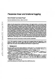
We consider an applications of the procedures presented in this paper. The US ex-post real interest rate series that has been studied in Bai and Perron (2003a) and Gonz´alez and Ter¨asvirta (2006), among others. The conclusions from these studies are that there are two to three breaks (or shifts) in the mean of the series. The US ex-post real interest rate is defined as the three-month treasury bill rate deflated by the consumer price index (CPI) inflation rate. Figure 2 presents the quarterly series containing 103 observations for the period 1961:1-1986:3. Looking at the series one may, indeed, suspect the presence of two or three breaks.

Figure 2: US ex-post real interest rate 1961:1 - 1986:3 Below we present the results from testing sequences at the 5% level of significance. If one is interested in finding out the number of changes only in the mean of the series, one should consider the test specification in Bai and Perron (2003a), that is identical to the Strategy (1) in Section 4.2.3. The only parameter to be tested for instability in this case is the intercept. Following BP, we set the minimum regime size to 15% of the total sample size, take care of serial correlation through pre-whitening and allow the residual variances be different across segments. As a result, we find three breaks, estimated at 1966:4, 1972:3 and 1980:3. To use any of the other strategies or the sequential procedure proposed in this paper, one has to choose the lag length k, initially assumed equal for every regime. It is selected from the linear autoregressive model using the Schwarz Bayesian information criterion and the Breusch-Godfrey LM test of no error autocorrelation. This results in the estimated lag length kˆ = 3. If we then follow Strategy (2) we detect three breaks at: 1967:2, 1974:3 and 1979:4. The number of breaks coincides with the results form Strategy (1), but the location of them does not. Following 17

Strategy (3) by relaxing the homogeneity restriction renders two breaks at 1974:3 and 1979:4. Given the nature of the series (changes in opposite directions) we would expect the testing sequence based on the third-order Taylor expansion have more power than the one based on the first-order expansion. For LM1 -based sequence the first p-value is equal to 0.485 and thus linearity is not rejected. LM3 -based test sequence is able to detect the nonlinearity. The p-value for the presence of a structural break is 0.0053 and the most prominent break found at 1979:4. At the second step, the linearity is again rejected, with p = 0.0134 and the second break is found at 1974:3. The third test in our sequence renders a p-value 0.048 and the presence of an additional break is rejected. If we would decide not to halve the significance level on each step the third p-value would signal the presence of another break. Summary of the results for all approaches considered can be found in Table 9.

6

Conclusions

In this paper we show how a smooth transition regression approximation to a piecewise linear structural break model is useful in determining the number of breaks in the latter model when it is not known in advance. The approach proposed and simulated in the paper is based on sequential hypothesis testing and is simple to apply in practice. The whole procedure is based on standard inference and the user can control the overall significance level of the tests in the sequence. In addition, no restrictions are imposed on the number of changing parameters. The simulations show that our procedure is well-sized and works well in comparison with the sequential procedure suggested by Bai and Perron. Neither of the alternatives dominates the other in small and moderate samples. The examples discussed above show that the results of both our and Bai and Perron’s approaches depend on the way the error autocorrelation is being taken care of. Adding lags to the model is a common practice, but sometimes small breaks can get absorbed by the extra dynamics. Then again, in practice a firm knowledge of the presence of a break is rather an exception than rule and a casual modeller would add lags to the model. One has to be careful when applying Bai and Perron’s technique as well. The results can depend heavily on the assumptions one is or is not willing to make about the error term and series at hand. Allowing for different distributions of covariates in different segments helps a great deal, but an unnecessary prewhitening 18

can considerably weaken the procedure’s ability to detect breaks. Overall, our ST-method can be considered a complement to the classical approach of Bai and Perron. Our procedure may be extended to accommodate heteroskedasticity by making the error variance change over time at the same points as the mean. This extension is, however, left for further research.

References Andrews, D. W. K. (1993). Tests for parameter instability and structural change with unknown change point. Econometrica 61, 821–856. Bai, J. (1997). Estimating multiple breaks one at a time. Econometric Theory 13, 315–352. Bai, J. (1999). Likelihood ratio tests for multiple structural changes. Journal of Econometrics 91, 299–323. Bai, J., R. L. Lumsdaine, and J. H. Stock (1998). Testing for and dating common breaks in multivariate time series. Review of Economic Studies 65, 395–432. Bai, J. and P. Perron (1998). Estimating and testing linear models with multiple structural changes. Econometrica 66, 47–78. Bai, J. and P. Perron (2003a). Computation and analysis of multiple structural change models. Journal of Applied Econometrics 18, 1–22. Bai, J. and P. Perron (2003b). Critical values for multiple structural change tests. Econometrics Journal 6, 72–78. Bai, J. and P. Perron (2006). Multiple structural change models: A simulation analysis. Econometric Theory and Practice: Frontiers of Analysis and Applied Research, D. Corbea, S. Durlauf and B. E. Hansen (eds.), Cambridge University Press. Ben A¨ıssa, M. S., M. Boutahar, and J. Jouini (2004). Bai and Perron’s and spectral density methods for structural change detection in the US inflation process. Applied Economics Letters 11, 109–115. Chow, G. C. (1960). Tests of equality between sets of coefficients in two linear regressions. Econometrica 28, 591–605. 19

Eitrheim, Ø. and T. Ter¨asvirta (1996). Testing the adequacy of smooth transition autoregressive models. Journal of Econometrics 74, 59–75. Goldfeld, S. M. and R. E. Quandt (1972). Nonlinear Methods in Econometrics. Amsterdam: North-Holland. Gonz´alez, A. and T. Ter¨asvirta (2006). Modelling autoregressive processes with a shifting mean. SSE/EFI Working Paper Series in Economics and Finance No. 637, Stockholm School of Economics. Lin, C.-F. and T. Ter¨asvirta (1994). Testing the constancy of regression parameters against continuous structural change. Journal of Econometrics 62, 211–228. Liu, J., S. Wu, and J. V. Zidek (1997). On segmented multivariate regressions. Statistica Sinica 7, 497–525. Luukkonen, R., P. Saikkonen, and T. Ter¨asvirta (1988). Testing linearity against smooth transition autoregressive models. Biometrika 75, 491–499. Prodan, R. (2006). Potential pitfalls in determining multiple structural changes with an application to purchasing power parity. Journal of Business and Economics Statistics. Forthcoming. Strikholm, B. and T. Ter¨asvirta (2005). Determining the number of regimes in a threshold autoregressive model using smooth transition autoregressions. SSE/EFI Working Paper Series in Economics and Finance No. 578, Stockholm School of Economics. Ter¨asvirta, T. (1994). Specification, estimation, and evaluation of smooth transition autoregressive models. Journal of the American Statistical Association 89, 208– 218. Ter¨asvirta, T. (1998). Modeling economic relationships with smooth transition regression. In A. Ullah and D. E. Giles (Eds.), Handbook of Applied Economic Statistics, pp. 507–552. Dekker, New York. Yao, Y.-C. (1988). Estimating the number of change-points via Schwarz’ Criterion. Statistics and Probability Letters 6, 181–189.

20

Tables Table 1: Selection frequencies of Bai and Perron sequential procedure (BP) and ST-procedures (LM1 and LM3 ). Data are generated with no breaks, i.e. m = 0. Model Choice m=0 (a) m=1 m=2

Uncorrected Corrected BP LM1 LM3 BPP W BP LM1 LM3 95.15 94.15 95.55 93.60 94.35 94.25 95.55 4.70 5.85 4.15 6.15 5.55 5.75 3.95 0.15 0.00 0.30 0.25 0.10 0.00 0.45

(b)

m=0 m=1 m=2

95.95 94.45 95.55 3.90 5.55 4.35 0.15 0.00 0.10

(c)

m=0 m=1 m=2

94.75 94.75 94.95 5.05 5.10 4.65 0.15 0.15 0.35

(d)

m=0 m=1 m=2

46.90 73.30 53.90 28.15 24.85 30.35 16.85 1.85 12.85

91.90 86.20 93.75 93.15 7.45 12.70 6.25 5.95 0.65 1.05 0.00 0.80

(e)

m=0 m=1 m=2

73.75 84.35 77.15 20.70 15.50 18.85 4.95 0.15 3.85

97.70 90.55 94.60 93.95 2.20 9.15 5.40 5.10 0.10 0.30 0.00 0.85

(f)

m=0 m=1 m=2

99.85 99.70 99.90 0.15 0.30 0.10 0.00 0.00 0.00

97.35 97.40 97.20 97.70 2.55 2.45 2.80 2.10 0.10 0.15 0.00 0.20

84.40 94.00 94.55 95.50 13.50 5.80 5.45 4.00 1.95 0.20 0.00 0.50

Notes: The table contains selection frequencies in per cent based on 2000 Monte Carlo replications. Columns labelled “Uncorrected” contain the results when not correcting for serial correlation, and columns labelled “Corrected” correspond to tests that correct for serial correlation either non-parametrically or parametrically. The column labelled “BPP W ” contains the results of the BP sequential test when prewhitening is applied before estimating the long-run covariance matrix. The columns labelled “LM1 ” and “LM3 ” correspond to the linearity tests that make use of the first-order and third-order Taylor expansions, respectively.

21

Table 2: Model selection frequencies of the uncorrected and corrected versions of the BP and ST-procedures. Data are generated from equation (10), i.e. errors are uncorrelated and m = 1. Uncorrected Model Choice BP LM1 LM3 Change in the intercept only: ν1 = ν2 = 1

Corrected BPP W BP

LM1

LM3

µ1 = 0 µ2 = 0.5 T = 120

m=0 m=1 m=2

55.75 46.50 58.80 42.60 52.90 39.90 1.60 0.55 1.20

36.75 44.25 47.00 59.65 54.65 53.95 52.35 38.80 8.00 1.80 0.65 1.20

µ1 = 0 (b) µ2 = 0.5 T = 240

m=0 m=1 m=2

20.20 14.90 25.25 77.85 83.40 73.40 1.95 1.65 1.35

14.25 13.60 15.35 25.75 78.00 84.60 83.25 72.90 7.70 1.75 1.40 1.30

µ1 = 0 µ2 = 1 T = 120

m=0 m=1 m=2

0.90 0.85 2.95 95.00 96.75 94.65 4.10 2.30 2.20

1.35 0.45 2.25 5.25 80.90 95.20 95.85 92.65 16.95 4.30 1.90 1.75

(a)

(c)

Change in the slope only: µ1 = µ2 = 0 ν1 = 1 (d) ν2 = 1.5 T = 120

m=0 m=1 m=2

21.85 15.40 26.75 75.45 83.15 71.25 2.65 1.45 1.95

11.55 14.75 15.85 27.10 73.50 82.30 82.80 70.80 14.35 2.95 1.30 1.80

ν1 = 1 ν2 = 1.5 T = 240

m=0 m=1 m=2

0.90 0.70 2.30 96.25 97.60 95.60 2.75 1.70 2.00

0.45 0.50 0.70 2.25 88.95 97.15 97.60 95.85 10.30 2.20 1.65 1.90

(e)

Change in all parameters: ν1 = 1, µ1 = 0 (f)

ν2 = 1.5 µ2 = 0.5 T = 120

m=0 m=1 m=2

0.30 0.30 1.10 95.75 97.15 96.40 3.90 2.40 2.30

0.10 0.15 0.45 1.55 82.15 95.20 97.30 96.20 17.00 4.60 2.25 1.95

(g)

ν2 = 2 µ2 = 1 T = 120

m=0 m=1 m=2

0.00 0.00 0.00 95.40 97.10 97.00 4.55 2.70 2.85

0.00 0.00 0.00 0.00 81.65 95.20 97.45 96.95 17.55 4.75 2.55 2.65

Notes: The table contains selection frequencies in per cent based on 2000 Monte Carlo replications. Columns labelled “Uncorrected” contain the results when not correcting for serial correlation, and columns labelled “Corrected” correspond to tests that correct for serial correlation either nonparametrically or parametrically. The column labelled “BPP W ” contains the results of the BP sequential test when prewhitening is applied before estimating the long-run covariance matrix. The columns labelled “LM1 ” and “LM3 ” correspond to the linearity tests that make use of the first-order and third-order Taylor expansions, respectively.

22

Table 3: Model selection frequencies of the uncorrected and corrected versions of the BP and ST-procedures. Data are generated from equation (11), i.e. errors are serially correlated and m = 1. Model µ1 = 0 (h) µ2 = 0.5 T = 120

Choice m=0 m=1 m=2

Uncorrected BP LM1 LM3 27.15 46.55 34.35 38.20 48.35 45.40 24.15 4.95 16.60

Corrected BPP W BP LM1 LM3 75.35 64.80 78.35 82.25 24.10 33.55 21.60 16.25 0.55 1.65 0.05 1.30

(i)

µ1 = 0 µ2 = 0.5 T = 240

m=0 m=1 m=2

14.85 30.00 23.05 41.25 60.50 51.20 26.60 9.15 20.25

62.30 52.05 62.60 71.60 36.60 46.05 37.20 26.30 1.05 1.85 0.20 1.70

(j)

µ1 = 0 µ2 = 1 T = 120

m=0 m=1 m=2

4.95 10.80 7.80 49.35 75.20 62.90 30.90 13.65 23.85

32.85 23.60 41.00 52.30 64.20 70.80 58.85 45.35 2.85 5.40 0.15 1.90

µ1 = 0 (k ) µ2 = 1 T = 240

m=0 m=1 m=2

0.40 1.40 0.75 43.85 80.20 66.60 32.75 17.45 25.85

8.15 5.00 11.15 19.10 89.05 89.80 86.50 77.75 2.75 5.15 2.35 2.65

Notes: The table contains selection frequencies in per cent based on 2000 Monte Carlo replications. Columns labelled “Uncorrected” contain the results when not correcting for serial correlation, and columns labelled “Corrected” correspond to tests that correct for serial correlation either nonparametrically or parametrically. The column labelled “BPP W ” contains the results of the BP sequential test when prewhitening is applied before estimating the long-run covariance matrix. The columns labelled “LM1 ” and “LM3 ” correspond to the linearity tests that make use of the first-order and third-order Taylor expansions, respectively.

23

Table 4: Model selection frequencies of the uncorrected and corrected versions of the BP and ST-procedures. Data are generated from equation (12), m = 2. Uncorrected Corrected Model Choice BP LM1 LM3 BPP W BP Change in the intercept only: ν1 = ν2 = ν3 = 1 79.90 16.90 3.10 0.10

m=0 m=1 m=2 m=3

57.60 8.90 31.30 2.15

µ1 = 0 µ2 = 1 µ3 = 2

m=0 m=1 m=2 m=3

0.00 0.00 0.00 41.50 47.50 64.95 55.10 52.05 34.30 3.20 0.45 0.75

0.00 0.00 0.00 0.40 25.05 31.40 67.25 79.70 72.85 68.15 32.50 19.20 2.10 0.45 0.25 0.70

µ1 = 0 (d) µ2 = 1 µ3 = −1

m=0 m=1 m=2 m=3

0.00 10.40 0.05 12.45 15.65 28.85 83.45 73.10 70.25 4.00 0.85 0.85

0.45 0.00 57.50 17.45 10.45 9.25 17.45 34.10 88.55 90.70 24.85 47.80 0.55 0.05 0.20 0.65

(e)

µ1 = 0 µ2 = −1 µ3 = 2

m=0 m=1 m=2 m=3

0.00 0.00 0.00 14.80 18.55 30.15 81.80 80.75 69.15 3.30 0.70 0.70

0.00 0.00 35.50 15.65 11.50 10.90 23.20 38.10 87.90 88.95 40.80 45.60 0.60 0.15 0.50 0.65

(f)

µ1 = 0 µ2 = 1 µ3 = 3

m=0 m=1 m=2 m=3

0.00 0.00 0.00 14.25 18.70 31.65 80.95 80.50 67.50 4.60 0.80 0.85

0.00 0.00 0.05 0.45 11.05 9.65 43.00 58.85 88.40 90.20 56.35 39.45 0.55 0.15 0.60 1.25

(g)

µ1 = 0 µ2 = 2 µ3 = −1

m=0 m=1 m=2 m=3

0.00 29.25 0.00 0.00 0.05 0.05 93.95 69.65 98.65 5.85 1.05 1.30

0.55 0.55 88.90 37.95 0.00 0.00 0.90 2.75 99.35 99.35 10.05 58.45 0.10 0.10 0.15 0.85

Notes: See the Notes of Table 3.

24

82.70 13.45 3.85 0.00

80.70 14.95 4.30 0.05

µ1 = 0 (b) µ2 = 1 µ3 = 0

97.15 29.60 1.40 27.40 1.40 42.60 0.05 0.40

70.10 17.65 11.55 0.70

95.30 4.55 0.15 0.00

88.90 9.60 1.50 0.00

(c)

95.10 4.70 0.20 0.00

LM3

m=0 m=1 m=2 m=3

(a)

µ1 = 0 µ2 = 0.5 µ3 = 0

LM1

52.00 57.25 6.45 6.55 40.10 36.10 1.45 0.10

97.55 39.25 1.55 24.40 0.90 35.95 0.00 0.40

Table 4: Model selection frequencies of the uncorrected and corrected versions of the BP and ST-procedures. Data are generated from equation (12), m = 2, (cont.). Uncorrected Model Choice BP LM1 LM3 Change in the slope only: µ1 = µ2 = µ3 = 0

Corrected BPP W BP

LM1

ν1 = 1 (h) ν2 = 1.5 ν3 = 1

m=0 m=1 m=2 m=3

78.05 14.35 7.25 0.35

95.30 60.65 4.05 25.85 0.60 13.15 0.05 0.35

58.60 74.45 13.90 14.00 26.15 11.45 1.35 0.10

95.35 61.35 3.85 23.30 0.80 15.20 0.00 0.15

ν1 = 1 (i) ν2 = 2 ν3 = 1

m = 0 20.05 m=1 1.25 m = 2 72.20 m=3 6.35

96.20 6.55 0.65 7.90 3.15 84.85 0.00 0.70

31.40 53.60 1.25 1.10 65.40 44.95 1.95 0.35

96.30 7.60 0.75 7.65 2.95 84.20 0.00 0.55

ν1 = 1 (j) ν2 = 1.5 ν3 = 2

m=0 0.25 0.10 m = 1 86.70 86.45 m = 2 12.55 13.45 m=3 0.50 0.00

ν1 = 1 (k) ν2 = 2 ν3 = 3

m=0 0.00 0.00 0.00 m=1 2.35 5.50 10.90 m = 2 89.50 93.60 88.30 m=3 7.75 0.90 0.80

0.00 0.00 0.00 0.00 2.05 3.40 7.35 13.40 94.10 95.45 91.90 85.70 3.85 1.15 0.75 0.90

m=0 0.00 0.00 0.00 m = 1 60.95 62.10 74.00 m = 2 37.50 37.45 25.55 m=3 1.55 0.45 0.45 Change in all parameters µ1 = 0, ν1 = 1 m = 0 87.85 94.40 79.40 5.40 17.25 (m) µ2 = 0.5, ν2 = 0.5 m = 1 10.55 µ3 = 0, ν3 = 1 m = 2 1.55 0.20 3.10 m=3 0.05 0.00 0.25

0.00 0.00 0.00 0.00 35.70 50.15 66.70 78.85 62.50 49.55 33.05 20.65 1.80 0.30 0.25 0.50

µ1 = 0, ν1 = 1 (n) µ2 = 1, ν2 = 1.5 µ3 = 2, ν3 = 2

m=0 0.00 0.00 0.00 m = 1 13.75 15.90 27.55 m = 2 83.70 83.15 71.65 m=3 2.55 0.95 0.80

0.00 0.00 0.00 0.00 13.50 9.65 17.80 30.75 86.15 90.35 81.50 68.55 0.35 0.00 0.70 0.70

µ1 = 0, ν1 = 1 (o) µ2 = 1, ν2 = 2 µ3 = 2, ν3 = 1

m=0 0.00 0.00 0.00 m = 1 16.20 20.40 30.45 m = 2 80.10 78.85 68.50 m=3 3.55 0.75 1.05

0.00 0.00 3.75 0.30 20.15 12.20 21.90 32.50 78.90 87.70 73.95 66.30 0.95 0.10 0.40 0.90

0.50 90.70 8.55 0.25

ν1 = 1 (l) ν2 = 0.5 ν3 = −0.5

Notes: See the Notes of Table 3.

25

0.30 0.50 0.10 56.30 75.85 87.20 42.15 23.55 12.65 1.25 0.10 0.05

76.20 15.85 7.60 0.35

82.05 14.70 3.20 0.05

94.60 5.20 0.20 0.00

LM3

0.55 91.35 7.85 0.25

79.55 15.95 4.30 0.20

Table 5: Model selection frequencies of the uncorrected and corrected versions of the BP and ST-procedures. Data are generated from equation (13), i.e. errors are serially correlated and m = 2. Choice m=0 (a) µ2 = 0.5 m = 1 T = 120 m = 2 m=3

Uncorrected BP LM1 LM3 37.65 74.30 43.10 25.20 22.90 31.55 22.45 2.70 21.20 10.75 0.10 4.15

m=0 (b) µ2 = 0.5 m = 1 T = 240 m = 2 m=3

27.45 22.25 27.00 16.45

75.05 35.05 19.50 31.35 5.20 28.25 0.25 5.35

87.75 9.35 2.90 0.00

(c) µ2 = 1 T = 120

m=0 m=1 m=2 m=3

18.75 14.15 32.80 24.45

(d) µ2 = 1 T = 240

Model

Corrected BPP W BP 88.75 82.50 9.90 14.30 1.35 3.20 0.00 0.00

LM1 94.95 5.05 0.00 0.00

LM3 88.40 8.90 2.40 0.30

82.10 12.55 5.35 0.00

95.45 4.55 0.00 0.00

84.70 11.05 4.15 0.10

77.15 22.05 14.20 25.15 7.95 43.90 0.70 8.90

81.80 74.75 11.95 14.85 6.15 10.30 0.10 0.10

97.45 2.55 0.00 0.00

79.05 13.15 7.45 0.35

m=0 m=1 m=2 m=3

4.20 77.95 7.40 5.20 6.95 12.35 39.55 14.05 64.95 33.10 1.05 15.30

67.85 64.90 12.40 11.35 19.55 23.40 0.20 0.35

97.80 57.80 2.05 19.25 0.15 22.80 0.00 0.15

(e) µ2 = 2 T = 120

m=0 m=1 m=2 m=3

0.35 85.35 1.30 0.65 1.45 2.00 39.05 11.50 75.35 38.50 1.70 21.35

75.85 78.05 2.90 2.15 20.90 19.55 0.35 0.25

99.80 63.15 0.20 9.35 0.00 27.25 0.00 0.25

(f) µ2 = 2 T = 240

m=0 m=1 m=2 m=3

0.00 85.55 0.00 0.00 0.00 0.05 35.60 12.15 75.25 37.65 2.30 24.70

34.30 59.80 0.05 0.00 64.90 39.95 0.75 0.25

99.80 21.05 0.10 4.75 0.10 73.45 0.00 0.75

(g) µ2 = 4 T = 120

m=0 m=1 m=2 m=3

0.00 0.00 37.50 38.90

96.95 0.00 0.00 0.00 2.25 72.75 0.80 27.25

92.70 0.00 7.30 0.00

99.25 100.00 74.00 0.00 0.00 1.20 0.75 0.00 24.05 0.00 0.00 0.75

(h) µ2 = 4 T = 240

m=0 m=1 m=2 m=3

0.00 0.00 36.35 37.55

96.80 0.00 0.00 0.00 2.35 72.40 0.85 27.60

48.30 0.00 51.70 0.00

98.10 100.00 45.35 0.00 0.00 0.10 1.90 0.00 53.15 0.00 0.00 1.40

Notes: See the Notes of Table 3.

26

Table 6: Model selection frequencies of the uncorrected and corrected versions of the BP and ST-procedures. Uncorrelated but heterogenous data and errors across segments, m = 2, ǫR = 0.15 for the corrected versions. Model

Uncorrected Choice BP LM1

LM3

AC-Correct BPP W BP

LM1

LM3

σi2 (u) BP

σ22 = 2 m=0 m=1 (a) ς2 = 2 T = 120 m = 2

0.00 20.85 11.45 13.35 83.90 65.30

0.00 23.80 75.60

0.70 1.00 23.75 30.70 56.80 65.65

42.90 32.40 24.45

5.35 0.00 55.10 6.20 39.25 91.95

σ22 = 2 m=0 (b) ς2 = 2 m=1 T = 240 m = 2

0.00 1.10 0.15 0.35 96.60 97.55

0.00 0.85 98.30

0.00 0.00 3.45 3.55 72.95 94.35

10.05 14.65 74.75

0.10 0.00 24.35 0.05 74.75 98.95

σ22 = 2 m=0 (c) ς2 = 4 m=1 T = 120 m = 2

0.00 24.30 25.85 39.40 70.35 36.10

0.00 41.50 57.75

12.60 63.60 19.45

7.90 87.20 4.85

30.20 57.45 12.20

1.65 0.00 71.50 9.45 26.30 88.75

σ22 = 2 m=0 (d) ς2 = 4 m=1 T = 240 m = 2

0.00 2.20 0.75 12.40 95.90 84.35

0.00 5.55 93.55

0.15 73.50 21.70

0.15 94.80 5.00

4.55 54.60 40.15

0.00 0.00 45.05 0.10 54.10 98.55

σ22 = 4 m=0 (e) ς2 = 2 m=1 T = 120 m = 2

0.00 34.70 33.10 24.80 62.70 40.35

0.30 44.40 54.65

1.95 3.10 35.45 50.30 47.70 45.10

57.15 31.10 11.75

14.80 0.00 59.50 19.80 25.35 78.80

σ22 = 4 m=0 (f) ς2 = 2 m=1 T = 240 m = 2

0.00 3.40 4.80 4.30 91.00 91.25

0.00 8.45 90.40

0.00 0.00 17.90 23.05 63.45 75.15

19.15 23.20 57.45

0.65 0.00 40.35 1.75 58.30 97.35

σ22 = 4 m=0 (g) ς2 = 4 m=1 T = 120 m = 2

0.00 36.05 51.55 45.35 44.75 18.50

0.15 62.30 36.90

31.00 47.35 18.25

19.05 76.70 4.25

46.95 47.45 5.60

7.60 0.00 76.95 17.80 15.25 79.80

σ22 = 4 m=0 (h) ς2 = 4 m=1 T = 240 m = 2

0.00 4.80 10.45 27.80 85.30 66.95

0.00 20.55 78.35

4.00 70.90 21.35

0.45 96.15 3.40

12.10 62.40 25.30

0.35 0.00 64.20 1.05 35.00 96.75

Notes: The table contains selection frequencies in per cent based on 2000 Monte Carlo replications. Columns labelled “Uncorrected” contain the results when not correcting for serial correlation, and columns labelled “AC-Correct” correspond to tests that correct for serial correlation either nonparametrically or parametrically. The column labelled “BPP W ” contains the results of the BP sequential test when prewhitening is applied before estimating the long-run covariance matrix. The column labelled “σi2 (u)” contains the results of the BP sequence when the correct specification of the test is applied. The columns labelled “LM1 ” and “LM3 ” correspond to the linearity tests that make use of the first-order and third-order Taylor expansions, respectively.

27

Table 7: Model selection frequencies of the uncorrected and corrected versions of the BP and ST-procedures. Uncorrelated but heterogenous data and errors across segments, m = 2. Model

Uncorrected Choice BP LM1

LM3

AC-Correct BPP W BP

LM1

LM3

σi2 (u) BP

σ22 = 2 m=0 0.00 0.00 0.00 m = 1 35.75 38.90 56.95 (a) ς2 = 2 T = 120 m = 2 60.35 60.50 42.55

0.05 0.00 0.00 41.15 59.25 51.80 56.70 40.65 48.05

0.00 0.00 67.65 21.80 32.00 78.00

σ22 = 2 m=0 0.00 0.00 0.00 (b) ς2 = 2 m=1 0.80 1.90 3.85 T = 240 m = 2 90.85 97.10 95.25

0.00 0.00 0.00 6.80 8.65 11.95 90.90 90.45 87.35

0.00 0.00 17.70 0.35 81.50 97.70

σ22 = 2 m=0 0.00 0.00 0.00 (c) ς2 = 4 m = 1 46.50 65.40 65.25 T = 120 m = 2 50.45 34.30 34.05

5.00 81.00 13.65

0.00 0.00 98.75 72.85 1.25 27.05

0.00 0.00 74.80 20.40 24.80 78.75

σ22 = 2 m=0 0.00 0.00 0.00 (d) ς2 = 4 m=1 2.15 20.75 10.45 T = 240 m = 2 93.35 78.70 88.70

0.00 83.25 16.60

0.00 0.00 99.00 42.05 1.00 57.45

0.00 0.00 31.60 0.15 67.85 99.20

σ22 = 4 m=0 0.00 0.00 0.10 (e) ς2 = 2 m = 1 75.00 75.00 86.50 T = 120 m = 2 22.55 24.10 12.90

0.85 0.20 0.00 61.05 86.80 79.55 37.00 12.95 20.40

0.25 0.00 88.75 58.90 10.65 41.10

σ22 = 4 m=0 0.00 0.00 0.00 (f) ς2 = 2 m = 1 17.35 17.70 34.10 T = 240 m = 2 75.80 81.35 64.45

0.00 0.00 0.00 35.95 51.40 29.95 62.30 48.55 69.80

0.00 0.00 49.65 8.75 49.45 90.50

σ22 = 4 m=0 0.00 0.05 0.00 (g) ς2 = 4 m = 1 76.80 84.55 84.70 T = 120 m = 2 20.25 14.95 14.25

15.60 71.95 12.20

0.00 0.05 99.35 87.40 0.65 12.55

0.00 0.00 87.85 36.10 11.70 63.15

σ22 = 4 m=0 0.00 0.00 0.00 (h) ς2 = 4 m = 1 23.75 49.30 40.50 T = 240 m = 2 71.00 50.45 57.90

1.75 81.05 16.85

0.00 0.00 99.55 60.55 0.45 39.35

0.00 0.00 54.80 2.00 44.20 95.70

Notes: See the Notes of Table 6.

28

Table 8: Model selection frequencies at 5% nominal level, data generated from (16). Choice m=0 m=1 m=2 m=3

BP(1) 0.00 27.55 72.00 00.45

BP(2) 0.00 3.40 23.95 24.75

BP(3) 0.00 5.85 86.05 7.45

LM1 29.75 10.60 59.10 1.40

LM3 0.65 21.35 76.80 1.20

Notes: The columns labelled “BP(i)”, i = 1, 2, 3, refer to the Strategy (i) on page 15. The columns labelled “LM1 ” and “LM3 ” correspond to the linearity tests that make use of the first-order and third-order Taylor expansions, respectively.

Table 9: Selected break dates for the US expost real interest rate series. BP(1)

BP(2)

BP(3)

1966:4 1972:3 1980:3

1967:2 1974:3 1979:4

1974:3 1979:4

LM1

LM3

1974:3 1979:4

Notes: The columns labelled “BP(i)”, i = 1, 2, 3, refer to the Strategy (i) on page 15. The columns labelled “LM1 ” and “LM3 ” correspond to the linearity tests that make use of the first-order and third-order Taylor expansions, respectively.

29