Deterministic Parallel DPLL (DP 2 LL) MSR-TR-2011-47 Youssef Hamadi1,2 , Said Jabbour3 , Cédric Piette3 , and Lakhdar Saïs3 1 2
Microsoft Research, Cambridge United Kingdom LIX École Polytechnique, F91128 Palaiseau, France
[email protected] 3 Université Lille-Nord de France, Artois, CRIL, CNRS UMR 8188, F-62307 Lens {jabbour,piette,sais}@cril.fr
Abstract. Parallel Satisfiability is now recognized as an important research area. The wide deployment of multicore platforms combined with the availability of open and challenging SAT instances are behind this recognition. However, the current parallel SAT solvers suffer from a non-deterministic behavior. This is the consequence of their architectures which rely on weak synchronizing in an attempt to maximize performance. This behavior is a clear downside for practitioners, who are used to both runtime and solution reproducibility. In this paper, we propose the first Deterministic Parallel DPLL engine. It is based on a stateof-the-art parallel portfolio architecture and relies on a controlled synchronizing of the different threads. Our experimental results clearly show that our approach preserves the performance of the parallel portfolio approach while ensuring full reproducibility of the results.
Keywords: SAT solving, Parallelism
1
Introduction
Parallel SAT solving has received a lot of attention in the last three years. This comes from several factors like the wide availability of cheap multicore platforms combined with the relative performance stall of sequential solvers. Unfortunately, the demonstrated superiority of parallel SAT solvers comes at the price of non reproducible results in both runtime and reported solutions. This behavior is the consequence of their architectures which rely on weak synchronizing in an attempt to maximize performance. Today SAT is the workhorse of important application domains like software and hardware verification, theorem proving, computational biology, and automated planning. These domains need reproducibility, and therefore cannot take advantage of the improved efficiency coming from parallel engines. For instance, a software verification tool based on a parallel SAT engine can report different bugs within different runtimes when executed against the same piece of code; an unacceptable situation for a software verification engineer. More broadly in science and engineering, reproducibility of the
results is fundamental, and in order to benefit to a growing number of application domains parallel solvers have to be made deterministic. More specifically, evaluating or comparing highly non-deterministic SAT solvers is clearly problematic. This problem led the organizers of the recent SAT race and competitions to explicitly mention their preferences for deterministic solvers and to introduce specific rules for the evaluation of parallel SAT solvers. For example, we can find the following statement at the SAT race 2008 "In order to obtain reproducible results, SAT solvers should refrain from using non-deterministic program constructs as far as possible. For many parallel solver implementations it is very hard to achieve reproducible runtimes. Therefore, this requirement does not apply to the parallel track. As runtimes are highly deviating for parallel SAT solvers, each solver was run three times on each instance. An instance was considered solved, if it could be solved in at least one of the three runs of a solver". For the parallel track, different evaluation rules are used in the SAT 2009 competition and SAT race 2010, illustrating the recurring problems of the evaluation of parallel SAT solvers. In this work, we propose a deterministic parallel SAT solver. Its results are fully reproducible both in terms of reported solution and runtime, and its efficiency is equivalent to a state-of-the-art non-deterministic parallel solver. It defines a controlled environment based on a total ordering of solvers’ interactions through synchronization barriers. To maximize efficiency, information exchange (conflict-clauses) and check for termination are performed on a regular basis. The frequency of these exchanges greatly influences the performance of our solver. The paper explores the trade off between frequent synchronizing which allows the fast integration of foreign conflict-clauses at the cost of more synchronizing steps, and infrequent synchronizing which avoids costly synchronizing at the cost of delayed foreign conflict-clauses integration. The paper is organized as follows. We detail the main features of modern sequential and parallel SAT solvers in Section 2 and provides motivation of this work in Section 3. Our main contribution is depicted in Section 4. In Section 5, our implementation is fully evaluated. Before the conclusive discussion in Section 7, a comprehensive overview of previous works is given in Section 6.
2 2.1
Technical Background Modern SAT solvers
The SAT problem consists in finding an assignment to each variable of a propositional formula expressed in conjunctive normal form (CNF). Most of the state-of-the-art SAT solvers are based on a reincarnation of the historical Davis, Putnam, Logemann, and Loveland procedure, commonly called DPLL [1]. A modern sequential DPLL solver performs a backtrack search; selecting at each node of the search tree, a decision variable which is set to a Boolean value. This assignment is followed by an inference step that deduces and propagates some forced unit literal assignments. This is recorded in the implication graph, a central data-structure, which records the partial assignment together with its implications. This branching process is repeated until finding a feasible assignment (model), or reaching a conflict. In the first case, the formula is answered to be satisfiable, and the model is reported, whereas in the second case, a conflict clause
(called asserting clause) is generated by resolution following a bottom-up traversal of the implication graph [2,3]. The learning process stops when a conflict clause containing only one literal from the current decision level is generated. Such a conflict clause (or learnt clause) expresses that such a literal is implied at a previous level. The solver backtracks to the implication level and assigns that literal to true. When an empty conflict clause is generated, the literal is implied at level 0, and the original formula can be reported unsatisfiable. In addition to this basic scheme, modern solvers use additional components such as an activity based heuristics, and a restart policy. Let us give some details on these last two important features. The activity of each variable encountered during each resolution process is increased. The variable with greatest activity is selected to be assigned next. This corresponds to the so-called VSIDS variable branching heuristic [3]. During branching after a certain amount of conflicts, a cutoff limit is reached and the search is restarted. The evolution of the cutoff value is controlled by a restart policy (e.g. [4]). Thanks to the activity of the variables cumulated during the previous runs, the objective of the restarts is to focus early (top of the tree) on important areas of the search space. This differs from the original purposes behind randomization and restarts introduced in [5]. For an extensive overview of current techniques to solve SAT, the reader is refered to [6]. 2.2
Parallel SAT solvers
There are two approaches to parallel SAT solving. The first one implements the historical divide-and-conquer idea, which incrementally divides the search space into subspaces, successively allocated to sequential DPLL workers. These workers cooperate through some load balancing strategy which performs the dynamic transfer of subspaces to idle workers, and through the exchange of interesting learnt clauses [7,8]. The parallel portfolio approach was introduced in 2008. It exploits the complementarity between different sequential DPLL strategies to let them compete and cooperate on the same formula. Since each worker deals with the whole formula, there is no need to introduce load balancing overheads, and cooperation is only achieved through the exchange of learnt clauses. With this approach, the crafting of the strategies is important, especially with a small number of workers. In general, the objective is to cover the space of good search strategies in the best possible way.
3
Motivations
As mentioned above, all the current parallel SAT solvers suffer from a non-deterministic behavior. This is the consequence of their architectures which rely on weak synchronizing in an attempt to maximize performance. Conflict-clauses sharing usually exploited in parallel SAT solvers to improve their performance accentuates even more their nondeterministic behavior i.e., non reproducibility in terms of runtime, reported solutions or unsatisfiability proofs. To illustrate the variations in terms of solutions and runtimes, we ran several times the same parallel solver ManySAT (version 1.1) [9] on all the satisfiable instances used
in the SAT Race 2010 and report several measures. Each instance was tested 10 times and the time limit for each run was set to 40 minutes. The obtained results are depicted in Table 3. For each instance, we give the number of variables (nbV ars), the number of successful runs (nbM odels) and the number of different models (diff) obtained by those runs. Two models are different if their hamming distance is not equal to 0. We ¯ H ¯ ¯ = also report the normalized average hamming distance nH nbV ars where H is the average of the pairwise hamming distance between the different models.
Instance 12pipe_bug8 ACG-20-10p1 AProVE09-20 dated-10-13-s gss-16-s100 gss-19-s100 gss-20-s100 itox_vc1138 md5_47_4 md5_48_1 md5_48_3 safe-30-h30-sat sha0_35_1 sha0_35_2 sha0_35_3 sha0_35_4 sha0_36_5 sortnet-8-ipc5-h19-sat total-10-19-s UCG-20-10p1 vmpc_27 vmpc_28 vmpc_31
nbVars 117526 381708 33054 181082 31248 31435 31503 150680 65604 66892 66892 135786 48689 48689 48689 48689 50073 361125 331631 259258 729 784 961
nbModels (diff) 10 (1) 10 (10) 10 (10) 10 (10) 10 (1) 10 (1) 10 (1) 10 (10) 10 (10) 10 (10) 10 (10) 10 (10) 10 (10) 10 (10) 10 (10) 10 (10) 10 (10) 4 (4) 10 (10) 10 (10) 10 (2) 10 (2) 8 (1)
¯ nH 0 1.42 33.84 0.67 0 0 0 26.62 34.8 34.76 34.16 22.32 33.18 33.25 32.76 33.2 34.19 15.86 0.5 2.12 2.53 3.67 0
avgTime (σ) 2.63 (53.32) 1452.24 (40.61) 19.5 (9.03) 6.25 (9.30) 38.77 (18.75) 441.75 (35.78) 681 (58.27) 0.65 (22.99) 173.9 (31.03) 704.74 (74.65) 489.02 (68.96) 0.37 (0.79) 45.4 (21.88) 61.65 (29.93) 72.21 (21.93) 105.8 (35.22) 488.16 (58.58) 2058.39 (47.5) 5.31 (6.75) 768.17 (31.63) 11.95 (32.62) 34.61 (25.92) 583.36 (88.65)
Table 1. Non-deterministic behavior of ManySAT
As expected, the solver exhibits a non-deterministic behavior in term of reported models. Indeed, on many instances, one can see that each run leads to a different model. ¯ For example, on the These differences are illustrated in many cases by a large nH. ¯ is around 30% i.e., sha0_ ∗ _∗ familly, the number of different models is 10 and the nH the models differ in the truth value of about 30% of the variables. Finally, the average time (avgT ime) and the standard deviation (σ) illustrate the variability of the parallel solver in term of solving time. The 12pipe_bug8 instance illustrates an extreme case. Indeed, to find the same model (diff =1) the standard deviation of the runtime is about
Algorithm 1: Deterministic Parallel DPLL
1 2 3 4 5 6 7
Data: A CNF formula F; Result: true if F is satisfiable; f alse otherwise begin answer[i] = search(corei ) ; for (i = 0; i < nbCores; i++) do if (answer[i]! = unknown) then return answer[i]; end
53.32 seconds while the average runtime value is 2.63 seconds. This first experiment clearly illustrates to which extent the non-deterministic behavior of parallel SAT solvers can influence the non reproducibility of the results.
4
Deterministic Parallel DPLL
In this section, we present the first deterministic portfolio based parallel SAT solver. As sharing clauses is proven to be important for the efficiency of parallel SAT solving, our goal is to design a deterministic approach while maintaining at the same time clause sharing. To this end, our determinization approach is first based on the introduction of a barrier directive () that represents a synchronization point at which a given thread will wait until all the other threads reach the same point. This barrier is introduced to synchronize both clauses sharing between the different computing units and termination detection (Section 4.1). Secondly, to enter the barrier region, a synchronization period for clause sharing is introduced and dynamically adjusted (Section 4.2). 4.1
Static Determinization
Let us now describe our determinization approach of non-deterministic portfolio based parallel SAT solvers. Let us recall that a portfolio based parallel SAT solver runs different incarnations of a DPLL-engine on the same instance. Lines 2 and 3 of the algorithm 1 illustrate this portfolio aspect by running in parallel these different search engines on the available cores. To avoid non determinism in term of a reported solution or an unsatisfiability proof, a global data structure called answer is used to record the satisfiability answer of these different cores. The different threads or cores are ordered according to their threads ID (from 0 to nbCores-1). Algorithm 1 returns the result obtained by the first core in this ordering who answered the satisfiability of the formula (lines 4-6). This is a necessary but not a sufficient condition for the reproducibility of the results. To achieve a complete determinization of the parallel solver, let us take a closer look to the DPLL search engine associated to each core (Algorithm 2). In addition to the usual description of the main component of DPLL based SAT solvers, we can see that two
Algorithm 2: search(corei )
1 2 3 4 5 6 7 8 9 10 11 12 13 14 15 16 17 18 19 20 21 22 23
Data: A CNF formula F; Result: answer[i] = true if F is satisfiable; f alse if F is unsatisfiable, unknown otherwise begin nbConflicts=0; while (true) do if (!propagate()) then nbConflicts++; if (topLevel) then answer[i]= f alse; goto barrier1 ; learntClause=analyze(); exportExtraClause(learntClause); backtrack(); if (nbConflicts % period == 0) then barrier1 : if (∃j|answer[j]! = unknown) then return answer[i]; updatePeriod(); importExtraClauses(); else if (!decide()) then answer[i]= true; goto barrier1 ; end
successive synchronization barriers (, lines 13 and 18) are added to the algorithm. To understand the role of these synchronizing points, we need to note both their placement inside the algorithm and the content of the region circumscribed by these two barriers. First, the barrier labeled barrier1 (line 13) is placed just before any thread can return a final statement about the satisfiability of the tested CNF. This barrier prevents cores from returning their solution (i.e. model or refutation proof) in an anarchic way, and forces them to wait for each other before stating the satisfiability of the formula (line 14 and 15). This is why the search engine of each core goes to the first barrier (labeled barrier1 ) when the unsatisfiability is proved (backtrack to the top level of the search tree, lines 6-8), or when a model is found (lines 20-22). At line 14, if the satisfiability of the formula is answered by one of the cores (∃j|answer[j]! = unknown), the algorithm returns its own answer[i]. If no thread can return a definitive answer, they all share information by importing conflict clauses generated by the other cores during the last period (line 17). After each one of them has finished to import clauses (second barrier, line 18), they continue to explore the search space looking for a solution. This second synchronization barrier is integrated to prevent each core from leaving the synchronization region before the others. In other words, when a given core enter this
second barrier, it waits for all other cores until all of them have finished importing the foreign clauses. As different clauses ordering will induce different unit propagation ordering and consequently different search trees, the clauses learnt by the other cores are imported (line 17) while following a fixed order of the cores w.r.t. their thread ID. To complete this detailed description, let us just specify the usual functions of the search engine. First, the propagate() function (line 4) applies classical unit propagation and returns false if a conflict occurs, and true otherwise. In the first case, a clause is learnt by the function analyze() (line 9), such a clause is added to the formula and exported to the other cores (line 10, exportExtraClause() function). These learned clauses are periodically imported in the synchronization region (line 17). In the second case, the decide() function choses the next decision variable, assigns it and returns true, otherwise it returns false as all the variable are assigned i.e., a model is found. Note that to maximize the dynamics of information exchange, each core can be synchronized with the other ones after each conflict, importing each learnt clause right after it has been generated. Unfortunately, this solution proves empirically inefficient, since a lot of time is wasted by the thread waiting. To avoid this problem, we propose to only synchronize the threads after some fixed number of conflicts period (line 10). This approach, called (DP )2 LL_static(period), does not update the period during search (no call to the function updateP eriod(), line 16). However, even if we have the "optimal" value of the parameter period, the problem of thread waiting at the synchronization barrier can not be completely eliminated. Indeed, as the different cores usually present different search behaviors (different search strategies, different size of the learnt databases, etc.), using the same value of the period for all cores, leads inevitably to wasted waiting time at the first barrier. In the next section, we propose a speed-based dynamic synchronization approach that exploits the current size of the formula to deduce a specific value of the period for each core (call to updateP eriod() function, line 16). 4.2
Speed-based Dynamic Synchronization
As mentioned above, the DPLL search engines used by the different cores develop different search trees, hence thread waiting can not be avoided even if the static value is optimally fine tuned. In this section, we propose a speed-based dynamic synchronization of the value of the period. Our goal is to reduce as much as possible the time wasted by the different cores at the synchronization barrier. The time needed by each core to perform the same number of conflicts is difficult to estimate in advance; however we propose an interesting approximation measure that exploits the current state of the search engine. As decisions and unit propagations are two fundamental operations that dominate the SAT solver run time, estimating their cost might lead us to a better approximation of the progression speed of each solver. More precisely, as the different cores are run on the same formula, to measure the speedup of each core, we exploit the size of its current learnt set of clauses as an estimation of the cost of these basic operations. Consequently, our speed-based dynamic synchronization of the period is a function of this important information. Let us formally describe our approach. In our dynamic synchronization strategy, for each core or computing unit ui , we consider a synchronization-time sequence as a
set of steps tki with t0i = 0 and tki = tk−1 + periodki where periodki represents the i time window defined in term of number of conflicts between tk−1 and tki . Obviously, i this synchronization-time sequence is different for all the computing units ui (0 ≤ i < nbCores). Let us define ∆ki as the set of clauses currently in the leant database of ui at step tki . In the sequel, when there is no ambiguity, we sometimes note tki simply k. Let us now formally describe the dynamic computation of these synchronizationtime sequences. Let m = max∀ui (|∆ki |), where 0 ≤ i < nbCores, be the size of the |∆k |
largest learnt clauses database and Sik = mi the ratio between the size of the learnt clauses database of ui and m. This ratio Sik represents the speedup of ui . When this ratio tends to one, the progression of the core ui is closer to the slowest core, while when it tends to 0, the core ui progresses more quickly than the slowest one. For k = 0 and for each ui , we set period0i to α, where α is a natural number. Then, at a given time step k > 0, and for each ui , the next value of the period is computed as follows: periodk+1 = α + (1 − Sik ) × α, where 0 ≤ i < nbCores. Intuitively, the core with i the highest speedup Sik (tending to 1) should have the lowest period. On the contrary, the core with the lowest speedup Sik (tending to 0) should have the highest value of the period.
5
Evaluation
period solving time waiting time waiting/solving time (in %) static(1) 10,276 4,208 40.9 static(100) 9,715 2,559 26.3 static(10000) 9,124 1,605 17.6 Table 2. Waiting time w.r.t. period synchronizing
All the experimentations have been conducted on Intel Xeon 3GHz under Linux CentOS 4.1. (kernel 2.6.9) with a RAM limit of 2GB. Our deterministic DPLL algorithm has been implemented on top of the portfolio-based parallel solver ManySAT (version 1.1). The timeout was set to 900 seconds for each instance, and if no answer was delivered within this amount of time, the instance was said unsolved. We used the 100 instances proposed during the recent SAT Race 2010, and we report for each experiment the number of solved instances (x-axis) together with the total needed time (y-axis) to solve them. Each parallelized solver is running using 4 threads. Note that in the following experiments, we consider the real time used by the solvers, instead of the classic CPU time. Indeed, in most architectures, the CPU time is not increased when the threads are asleep (e.g. waiting time at the barriers), so taking the CPU time into account would give an illegitimate substantial advantage to our deterministic solvers.
Sequential ManySat 1.1 (DP)2LL_static(1) (DP)2LL_static(100) (DP)2LL_static(10000)
cumulated time (seconds)
10000
8000
6000
4000
2000
0 50
55
60 65 #solved instances
70
75
Fig. 1. Performances using static synchronizing
5.1
Static Period
In a first experiment, we have evaluated the performance of our Deterministic Parallel DPLL ((DP )2 LL) with various static periods. Figure 1 presents the obtained results. First, a sequential version of the solver has been used. Unsurprisingly, this version obtains the worst global results by only solving 68 instances in more than 11,000 seconds. This result enables to show the improvement obtained by the use of parallelized engines. We also report the results obtained by the non-deterministic solver ManySAT 1.1. Note that as shown in Section 3, executing several times this version may lead to different results. This non-deterministic solver has been able to solve 75 instances within 8,850 seconds. Next, we ran a deterministic version of ManySAT where each core synchronizes with the other ones after each clause generation ((DP)2LL_static(1)). We can observe that the synchronization barrier is computationally heavy. Indeed, the deterministic version is clearly less efficient than the non-deterministic one, by only solving 72 instances out of 100 in more than 10,000 seconds. This negative result is mainly due to the time wasted by the cores waiting for each others on a (very) regular basis. To overcome this issue, we also tried to synchronize the different threads only after a given number of conflicts (100, 10000). Figure 1 shows that those versions outperform the "period=1" one, but they stay far from the results obtained by the non-deterministic version. The barriers that enable our algorithm to be deterministic are clearly a drawback to its efficiency. Therefore, we evaluated the amount of time spent by the threads waiting for each others. In Table 2, we report the rate of time spent waiting for synchronization with respect to the total solving time for the different versions of (DP)2LL. As the results show, this waiting time can be really significant when waiting after each conflict.
Indeed, in this case, more than 40% of the time is spent by the threads waiting for each other. As expected, this rate is reduced when the synchronization is achieved less often, but is never insignificant. Note that even if the "period=10000" version wastes less time than "period=100" waiting, it obtains worst global results by only solving 72 instances. The "period=100" version obtains the best results (discarding the non-deterministic version). Based on extensive experiments, this parameter seems to be a good tradeoff between the time spent at the barrier, and the dynamics of information exchange. Indeed, we believe that information is exchanged too late in the "period=10000" version, which explains its less satisfying behavior. Accordingly, we tried to reduce the waiting time of the threads by adopting a Speedbased dynamic strategy (presented Section 4.2). Empirical results about this dynamic technique are presented in the next section. 5.2
Dynamic Period
In a second experiment, we tried to empirically evaluate our dynamic strategy. We compare the results of this version with the ones obtained by ManySAT 1.1, and with the results of the best static version (100), and of the sequential one too. The results are reported in Figure 2. The dynamic version is run with parameter α = 300.
Sequential ManySat 1.1 (DP)2LL_static(100) (DP)2LL_dynamic
cumulated time (seconds)
10000
8000
6000
4000
2000
0 50
55
60 65 #solved instances
70
75
Fig. 2. Performance using dynamic synchronizing
This experiment empirically confirms the intuition that each core should have a different period value, w.r.t. the size of its own learnt clauses database, which heuristically indicates its unit propagation speed. Indeed, we can observe in Figure 2 that the "solving curve" of this dynamic version is really close to the one of ManySat 1.1. This
means that the 2 solvers are able to solve about the same amount of instances within about the same time. Moreover, this adaptive version is able to solve 2 more instances than the non-deterministic one, which makes it the most efficient version tested during our experiments.
6
Previous Works
In the last two years, portfolio based parallel solvers became prominent, and we are not aware of a recently developed divide-and-conquer approach (the latest being [8]). We describe here all the parallel solvers qualified during the 2010 SAT Race4 . We believe that these parallel portfolio approaches represent the current state-of-the-art in parallel SAT. In plingeling, [10] the original SAT instance is duplicated by a boss thread and allocated to worker threads. The strategies used by these workers are mainly differentiated by the amount of pre-processing, random seeds, and variables branching. Conflict clause sharing is restricted to units which are exchanged through the boss thread. This solver won the parallel track of the 2010 SAT Race. ManySAT [9] was the first parallel SAT portfolio. It duplicates the instance of the SAT problem to solve, and runs independent SAT solvers differentiated on their restart policies, branching heuristics, random seeds, conflict clause learning, etc. It exchanges clauses through various policies. Two versions of this solver were presented at the 2010 SAT Race, they finished respectively second and third. In SArTagnan, [11] different SAT algorithms are allocated to different threads, and differentiated with respect to, restarts policies, and VSIDS heuristics. Some threads apply a dynamic resolution process [12], or exploit reference points [13]. Some others try to simplify a shared clauses database by performing dynamic variable elimination or replacement. This solver finished fourth. In Antom, [14] the SAT algorithms are differentiated on decision heuristic, restart strategy, conflict clause detection, lazy hyper binary resolution [12], and dynamic unit propagation lookahead. Conflict clause sharing is implemented. This solver finished fifth.
7
Discussion
In this paper, we tackle the important issue of non determinism in parallel SAT solvers by proposing (DP )2 LL, a first implementation of a deterministic parallelized procedure for SAT. To this purpose, a simple but efficient idea is presented; it mainly consists in introducing two synchronization barriers to the algorithm. We propose different synchronizing strategies, and show that this deterministic version proves empirically very efficient; indeed, it can compete against a recent non-deterministic algorithm. This first implementation opens many interesting research perspectives. First, the barrier added to the main loop of the parallelized CDCL for making the algorithm deterministic can be seen as a drawback of the procedure. Indeed, every thread that has 4
http://baldur.iti.uka.de/sat-race-2010
terminated its partial computation has to wait for the all other threads to finish. Nevertheless, our synchronization policy proves effective while keeping the heart of the parallelized architecture: clause exchanges. Moreover, we think that it is possible to take even better advantage of this synchronization step. New ways for the threads of execution to interact can be imagined at this particular point; we think that this is a promising path for future research.
References 1. Davis, M., Logemann, G., Loveland, D.W.: A machine program for theorem-proving. Communications of the ACM 5(7) (1962) 394–397 2. Marques-Silva, J., Sakallah, K.: GRASP - A New Search Algorithm for Satisfiability. In: ICCAD. (1996) 220–227 3. Zhang, L., Madigan, C., Moskewicz, M., Malik, S.: Efficient conflict driven learning in boolean satisfiability solver. In: ICCAD. (2001) 279–285 4. Biere, A.: Adaptive restart strategies for conflict driven SAT solvers. In: SAT. (2008) 28–33 5. Gomes, C., Selman, B., Kautz, H.: Boosting combinatorial search through randomization. In: AAAI. (1998) 431–437 6. Biere, A., Heule, M.J.H., van Maaren, H., Walsh, T., eds.: Handbook of Satisfiability. Volume 185 of Frontiers in Artificial Intelligence and Applications. IOS Press (2009) 7. Chrabakh, W., Wolski, R.: GrADSAT: A parallel SAT solver for the grid. Technical report, UCSB Computer Science (2003) 8. Chu, G., Stuckey, P.J.: Pminisat: a parallelization of minisat 2.0. Technical report, SAT Race (2008) 9. Hamadi, Y., Jabbour, S., Sais, L.: ManySAT: a parallel SAT solver. Journal on Satisfiability, Boolean Modeling and Computation 6 (2009) 245–262 10. Biere, A.: Lingeling, plingeling, picosat and precosat at SAT race 2010. Technical Report 10/1, FMV Reports Series (2010) 11. Kottler, S.: SArTagnan: solver description. Technical report, SAT Race 2010 (July 2010) 12. Biere, A.: Lazy hyper binary resolution. Technical report, Dagstuhl Seminar 09461 (2009) 13. Kottler, S.: SAT solving with reference points. In: SAT. (2010) 143–157 14. Schubert, T., Lewis, M., Becker, B.: Antom: solver description. Technical report, SAT Race (2010)