the precision agriculture system plan for implementation on the field, relying on this productivity ... nomics at the University of Missouri-Columbia in Co- lumbia ...
Development of a conservation-oriented precision agriculture system: Crop production assessment and plan implementation N.R. Kitchen, K.A. Sudduth, D.B. Myers, R.E. Massey, E.J. Sadler, R.N. Lerch, J.W. Hummel, and H.L. Palm ABSTRACT: From site-specific crop and soil information collected from a Missouri claypan soil field for over a decade (1993 to 2003), we implemented a precision agriculture system in 2004 with a goal of using site-specific management practices to improve farming profitability and conserve soil and water resources. The objectives of this study were to: 1) show how precision crop and soil information was used to assess productivity, and 2) document the development of the precision agriculture system plan for implementation on the field, relying on this productivity assessment and conservation opportunities. The study field was uniformly managed from 19912003, during which time variability in soil and landscape parameters and yield were measured, and causes of yield variation were determined. Profitability maps were created from yield maps and production records. Because erosion has degraded the topsoil on shoulder and side slope positions of major portions of this field, corn-soybean management practices have rarely been profitable in these shallow topsoil areas. We prioritized these and other results, and developed the precision agriculture system plan. The plan, described in detail, is aimed at increasing profitability while improving water and soil quality. Keywords: Precision agriculture system, profitability mapping, site-specific management, topsoil depth, yield limiting factors
“History is the science of what never happens twice” (Paul Valery, critic and poet, 1871 - 1945). Few will argue against the assertion that a historical perspective— even when it is not exactly the same twice— provides a valid foundation for projecting the potential consequences of future decisions. When considering the history of an individual crop production field and how it performs in food, forage, or fiber production, usually little or no record has been maintained describing the interplay of management practices, soil and land resources, and climate. This historical void can be effectively filled with the technologies and methods of precision agriculture. Precision agriculture has been defined as the application of technologies and principles to manage spatial and temporal variability associated with all aspects of agricultural
Reprinted from the Journal of Soil and Water Conservation Volume 60, Number 6 Copyright © 2005 Soil and Water Conservation Society
production (Pierce and Nowak, 1999). Precision agriculture has the capacity to enhance production and protect the environment while conserving soil and water resources. From this premise, Berry et al. (2003) developed the idea of ‘precision conservation,’ which was defined as the use of Newell R. Kitchen, Kenneth A. Sudduth, Edward J. Sadler, Robert N. Lerch, and John W. Hummel all work for the U.S. Department of Agriculture Agricultural Research Service, Cropping Systems and Water Quality Research Unit at the University of MissouriColumbia in Columbia, Missouri. D. Brenton Myers works in the Department of Soil, Environmental and Atmospheric Sciences at the University of MissouriColumbia in Columbia, Missouri. Raymond E. Massey works in the Department of Agricultural Economics at the University of Missouri-Columbia in Columbia, Missouri. Harlan L. Palm works in the Department of Agronomy at the University of Missouri-Columbia in Columbia, Missouri.
N| D 2005
VOLUME 60 NUMBER 6
421
precision technologies and procedures, across spatial and temporal variability, to achieve conservation objectives. They further proposed that precision conservation ties efforts across scales (zones within field to between fields to watershed and basin management) and is a key tool in achieving conservation goals. In this paper, we use a well-analyzed case study field to support the proposal that precision agriculture information can provide a historical perspective enabling simultaneous improvements in production profitability and conservation goals (for this paper, we use “conservation” to include aspects of environmental protection). The logic of tailoring management in time and space so that production inputs are provided as needed is convincing, even for non-agriculturally minded people. Yet, the producer’s primary justification for employing precision agriculture is to improve crop performance (Kitchen et al., 2002) while the public sector’s primary interest in precision agriculture is improving the environment (Vanden Heuvel, 1996). These should not be viewed as mutually exclusive objectives (Berry et al., 2003). Precision agriculture has been touted as “agriculture of the future” by which production profitability will be increased, agrichemical use will be reduced, nutrient use efficiencies will be increased, and off-field movement of soil and agrichemicals will be reduced (Larson et al., 1997). Precision agriculture should be promoted to the extent it facilitates conservation and production better than whole-field, conventional management practices. However, only a few studies have been conducted to determine whether these management strategies meet this high expectation. Most field-level studies have been either computer modeldriven comparisons, or statements of reduced loadings with precision applications (see literature reviews in Larson et al., 1997; Pierce and Nowak, 1999; Bongiovanni and Lowenberg-Deboer, 2004). Further, these studies typically focus on only one or two management practices/inputs when comparing site-specific management to uniform management. Results from these studies have been mixed. Often the likelihood that a precision agriculture approach improved production and/or environmental parameters was dependent on the degree and type of variability initially found in the experimental area. Some studies have found that the decision rules developed for uniform
422
JOURNAL OF SOIL AND WATER CONSERVATION N| D 2005
management were insensitive to management recommendations when developing a sitespecific plan (Ferguson et al., 2002). For some aspects of management [e.g., nitrogen (N)], seasonal climate influences have had more impact on production than spatial field variability, and thus temporal information may dictate the optimal management (Dinnes et al., 2002; Power and Weise, 2001). Conservation must be compatible with profitability. Otherwise, it will not be adopted and can not be sustainable in a free market economy. To achieve sustainable food production systems, it has been proposed that precision agriculture technologies and practices need to be integrated into conservation planning, in order to deal with the complexity of spatial heterogeneity of farmlands (Berry et al., 2003). Research demonstrating this integration in field-scale studies is lacking, in large part because of the time and expense required to conduct these types of studies. In 1991, we began collecting crop, soil, and water quality information on a typical claypan-soil field in Missouri. By 1993 our research investigations included measuring spatially-variable soil and crop information. Using information collected from this field for over a decade (1993, to 2003), we implemented the precision agriculture system for this field in 2004. The goal of this precision agriculture system is to use sitespecific management practices to improve profitability and to better protect soil and water resources as compared to past management practices. The objectives of this study were to: 1) show how precision information was used to assess crop productivity and profitability for this study field, and 2) document the development of the precision agriculture system plan, which relied on this productivity assessment along with the conservation opportunities described in Lerch et al. (2005). Methods and Materials The 36-ha (89 ac) study field and its management history are described in detail in Lerch et al. (2005). A major objective during 1993 to 2003 was to measure and map the variability of a number of different soil and crop properties with management practices being held constant on the field (i.e., conventional uniform management). Order 1 soil surveys (1:5,000 scale) were conducted on this field in 1993 and 1997 as described in Fraisse et al. (2001a). Apparent soil electrical conductivity (ECa) measure-
ments were obtained using the Veris (Veris Technologies Inc., Salina, Kansas) model 3100 sensor cart system and a mobile Geonics (Geonics Limited, Mississauga, Ontario, Canada) model EM-38 system (Sudduth et al., 2003). With the Veris 3100 sensor, both shallow [0 to 30 cm (0 to 12 in)] and deep [0 to 100 cm (0 to 39 in)] data were collected. The EM-38 sensor was operated in the vertical dipole mode, providing an effective measurement depth of 0 to 150 cm (0 to 59 in). Data from both sensors were collected on 10 m (33 ft) transects at 1 Hz, and georeferenced using differential global positioning system receivers. Elevation data from a real-time kinematic (vertical accuracy 3 to 5 cm or 1.18 to 1.97 in) global positioning system survey were collected on 10 m (33 ft) transects (Kitchen et al., 2005). The data were kriged in order to create a digital elevation model on a 10 m grid. Slope, profile curvature and aspect were then calculated from this digital elevation model using terrain modeling algorithms (Surfer v7, Golden Software Inc., Golden, Colorado). In odd years starting in 1993, soil was sampled for nutrients on a 30-m grid. Additional random sample points were included to assess short range variability (total samples = 468). Three (1993 only) or eight (1995-2003) cores were taken to a depth of 20 cm (8 in) within a 1-m (3-ft) radius of the differential-GPS referenced sampling point and composited. Samples were analyzed for phosphorus, potassium, cation exchange capacity (sum of bases), organic matter, and pH (Brown and Rodriguez, 1983). Only a field-average yield was available for 1991 and 1992. Starting in 1993, combine harvesters equipped with commerciallyavailable yield sensing systems were used to obtain yield data. Yield data points deemed questionable or unreliable because of errors or other operational problems were removed as discussed in Kitchen et al. (2003). While the methods and sampling intensity varied for the different measurements, we have applied standard geostatistical procedures for interpolation by kriging, mapping to a 10 × 10 m (33 × 33 ft) grid cell size, and extraction of mapped data as described in Kitchen et al. (2005). Subsequent analyses were conducted on all 10-m (33-ft) grid data, with the exception of soil fertility, where only the 10-m grids coincident with soil sample points were used. Correlation, regression, non-linear neural
Table 1. Monthly growing-season precipitation for the study field compared to the 56-year average (1948 to 2003). Year
Crop
1991 1992 1993 1994 1995 1996 1997 1998 1999 2000 2001 2002 2003 56-yr average
corn soybean corn soybean sorghum soybean corn soybean corn soybean corn soybean corn
Apr
May
Jun
Jul
Aug
Sep
Total
——————————————————— cm ——————————————————————— 9.1 15.0 4.0 15.4 4.8 11.7 60.0 6.4 2.3 2.4 14.8 2.6 8.1 36.6 14.5 8.6 14.2 16.2 13.2 36.0 102.7 26.4 2.6 8.9 1.0 3.9 6.0 48.8 13.7 25.7 17.3 7.4 16.8 7.3 88.2 6.2 17.4 8.8 7.0 12.2 8.6 60.2 8.2 12.6 9.9 4.0 9.1 5.6 49.4 10.3 5.5 24.0 14.9 4.2 14.2 73.1 17.5 8.6 14.0 0.9 3.4 3.1 47.5 2.2 8.6 17.1 7.1 22.3 4.7 62.0 11.5 18.5 15.4 8.9 2.1 5.0 61.4 13.9 23.3 5.3 5.4 8.6 1.5 58.0 10.3 13.8 16.4 1.7 8.5 12.5 63.2 8.9 10.8 10.8 9.0 8.9 9.2 57.6
network, cluster analysis, and boundary line analysis were used to analyze the compiled data layers (Sudduth et al., 1996; Kitchen et al., 1999; Fraisse et al., 2001a; Sudduth et al., 2003, Drummond et al., 2003; Kitchen et al., 2005). Profitability assessment. Profitability maps were generated from yield maps. A profit map is a comprehensive measure of field performance since it is an outcome that considers all resources spent and revenue received. Unlike yield maps, profit maps allow different crops to be compared by expressing them in a common metric. Profit maps were generated by subtracting input costs/expenses from gross revenue. Creating the profit map required the development of budgets for each grid cell where yield was measured and inputs recorded. Revenues and expenses were allocated to the year and crop that they benefited rather than the year in which they were incurred. Because the objective of profit mapping was to present actual profit rather than to make a forecast, actual grain prices were assigned as the higher of the appropriate loan rate or the average harvest time price (September to November) in the year of harvest (USDA, 2003). By using actual prices received, the profit map took into account market influences. Actual prices paid for inputs were also used in the profit map generation. Detailed records of field activities such as cultivating, planting, and spraying were maintained along with records of quantities and costs of all inputs used. The costs of field activities were estimated using published local custom rates (Plain et al., 2001). Land was charged the average rental price associated with each crop
year, based on statistics for the local crop reporting district (Plain and White, 2003). Overhead costs that are fixed with respect to acreage and yield, such as barns and computer expenses, were excluded from this analysis. A wage for field activities performed was included in the accounting of field activities (i.e., included in custom rates). No government program payments, other than loan rate, were considered as income. Profit maps were calculated by multiplying yield by price and subtracting the costs of field activities and inputs on a cell-by-cell basis. Because management was uniform, the cost of field activities and inputs was constant across the entire field. The gross revenue and hence, net revenue, varied as yield varied by location. Results and Discussion Crop production and soil properties. Year-toyear variation in yield was significant and was largely attributed to the amount of rainfall received in July and August ( Jung et al., 2005) (compare Table 1 with yield maps in Figure 1). In general, when total rainfall for the July-August period fell below 15 cm (5.91 in), crop stress occurred due to water deficiency, reducing grain yield. Claypan soils have relatively low drought tolerance because the high-clay subsoil has low plant-available water content (USDA-NRCS, 1995). Spatial variability in yield was extreme for most years, with the highest yielding areas 200 to 600 percent greater than the lowest yielding areas (Figure 1 yield map). Historically, variations in soil productivity have often been represented by soil type maps. Highly detailed Order 1 soil surveys
may provide information at the spatial resolution required to interpret sub-field variation in productivity (Figure 1). Visual examination of the data presented in Figure 1 verifies that yield patterns for many years have some similarity to soil survey, elevation, and/or ECa maps. We found that productivity variation on this field could be better represented by zones developed with a combination of ECa and topography data than with an Order 1 map (Fraisse et al., 2001a). However, using zones derived from these relatively static soil data still only represented less than or equal to 30 percent of the within-field yield variation, suggesting that other (e.g., pests, diseases, nutrients) variables were also affecting yield. Kitchen et al. (1999) confirmed this observation by using a boundary line analysis to quantify the relationship of yield to ECa in the absence of other yield-limiting factors. The interpretation of boundary line results varied from year to year depending on the climate and crop. As might be expected, the relationship between ECa and topography with yield also coincided with historic erosion patterns that largely dictate the soil quality status of this field (Lerch et al., 2005). East-west striping patterns seen in fertility, pH, and yield maps (Figure 3) were residual effects of the way this field has been managed in the past. Prior to 1990, the field was managed as a set of smaller fields. A visual comparison of the historical aerial photos (Lerch et al., 2005), fertility, and yield maps shows some similarity. As an example, an area of higher pH north of the east-west tree line is quite different from the rest of the field and is associated with higher yield seen in some yield maps (see 1993, 1994 and 1997).
N| D 2005
VOLUME 60 NUMBER 6
423
Figure 1 Maps showing variability in soil properties and crop yield for the study field. High and low values on legends adjacent to yield maps represent +/three standard deviations from the mean. Soybean yield legends range from 0.5 to 4.2 Mg ha-1 and corn yield legends range from 0.0 to 10.6 Mg ha-1.
Elevation
Order 1 soil survey* m
Aaqll
Aabll
ms m-1 2
Pt 261
Le Er
Deep ECa
Shallow ECa†
CEC‡ cmol[+] kg-1
ms m-1 2
9.5
Aaqll
Mex Le
Ad Le
Aabll
Ad
Ad
Le Er Mex
Pt
Pt
Pt 265
19
Organic matter % O.M. 1.4
pH s -log[H+] 4.6
21.4
45
Phosphorous
Potassium kg ha-1 74
kg ha-1 8
95 Sorghum -1
Mg ha
2.6
7.5
3.2
7.1
94 Soybean Mg ha-1 0.5
108
96 Soybean Mg ha-1
306
98 Soybean
00 Soybean Mg ha-1
Mg ha-1
02 Soybean Mg ha-1 0.9
1.3
1.5
2.0 2.9
2.8
3.1 3.6
4.2
93 Corn Mg ha-1
97 Corn Mg ha-1
99 Corn Mg ha-1
01 Corn Mg ha-1
0.6
03 Corn Mg ha-1 0.0
3.4
3.7 4.0
4.7 6.0 8.8
10.6
10.4 *
Aabll – Argialbolls Aaqll – Argiaquolls Ad – Adco Le – Leonard
†
EC = electrical conductivity. CEC = cation exchange capacity.
‡
424
JOURNAL OF SOIL AND WATER CONSERVATION N| D 2005
Le Er – Leonard eroded Mex – Mexico Pt – Putnam
Figure 2 However, in the majority of the years, spatial patterns in fertility maps bear little resemblance to patterns of yield variability. Correlations between yield and soil fertility measurements were generally low (|r| less than 0.20) and inconsistent from year to year (Sudduth et al., 1996; Kitchen et al., 1999). Therefore, including measured soil nutrient data along with topography and ECa provided little improvement in yield estimations using linear regression techniques. Better results were obtained with nonlinear nonparametric techniques, including projection pursuit regression and neural network analysis. These techniques allowed the analysis to consider complex non-linearities and interactions among variables that could not be modeled in linear regression. Neural networks were the most successful in modeling within-season yield variations, with r2 ≈ 0.60 in several cases (Sudduth et al., 1996; Drummond et al., 2003). Climate variables were not successful in generalizing the neural network yield estimation across multiple years. The complex nature of the climatesoil-topography interactions on this field would require numerous additional site-years of input data to develop models predictive of yield variations across a range of climatic conditions (Drummond et al., 2003). Overall, our research investigating yieldlimiting factors on this field has demonstrated that 1) because of their effect on soil water holding capacity and within field water redistribution, soil texture and topsoil depth (as inferred by ECa) and topography had the most persistent relationships with yield, although the shape of the relationship was dependent on the climate during the particular growing season; 2) relationships of yield variations to soil fertility variations were, in general, not strong; and 3) it was possible to model spatial yield variations within a single season using nonlinear techniques, but attempts to integrate climate measurements for a multi-year analysis were not successful. Production shown as profitability. Corn, soybean, and 10-year (1993 to 2002) average profitability maps for this field are presented in Figure 2. The balanced distribution of positive (greens) and negative (browns) profitability reflects the average profitability being nearly $0 per hectare over the 10 years of this analysis. The soybean map indicates that, on average, soybean profitability was positive over most of the field while the corn map indicates that, on average, corn profitability
Profitability of the average of four corn years (left), five soybean years (center), and ten years (2003 to 2002) (right) for the study field.
Soybean
Corn
All crops
$ ha-1 (67 - 90) (45 - 67) (34 - 45) (22 - 34) (17 - 22) (11 - 17) (6 - 11) (1 - 6) (1) - 1 1-6 6 - 11 11 - 17 17 - 22 22 - 34 34 - 45 45 - 67 67 - 90
0
55 110
220
330
N
Meters 440
was negative over most of the field. The overall financial loss with corn raises the question of whether or not corn should be grown on the field. While the corn profit map makes the question visually obvious, geo-referenced profit maps are not required to answer the question. The decision of whether or not a specific crop should be grown can be answered by looking at the profitability of the whole field. Other information, such as weather or pest pressure, might temper conclusions based on simple averages. For example, during several seasons when corn was grown on the field the crop experienced either July or August rainfall that was well below the longterm average (Table 1). The power of profit maps lies in their ability to indicate where,
within a field, all crops or a particular crop performed well or poorly. Profitability patterns persist over years as impacted by permanent features of the landscape. A drainage waterway runs northsouth through the middle of the field. The average profit map indicates that the land immediately adjacent to the drainage way was profitable for almost its entire length. Field drainage paths control sediment, nutrient, and agrichemical movement. As such they are frequent targets for application of conservation practices such as grassed waterways. The potential economic and conservation impacts of constructing a grass waterway for this field are discussed later. A soil feature that has had major negative
Figure 3 Graphical representation of the priorities chosen for the precision agriculture system. Highest priorities are on the bottom.
Ground water quality
1. decrease nitrates
Soil quality (sustainability)
1. greatly reduce topsoil loss 2. improve soil structure to enhance infiltration 3. build organic matter
Surface water quality
1. reduce sediment loss 2. reduce herbicide loss 3. reduce nutrient loss 1. reduce cost 2. achieve stable yield 3. improve water use efficiency
Production (profitability)
N| D 2005
VOLUME 60 NUMBER 6
425
impact on profitability is low topsoil thickness (seen as high ECa areas in Figure 1 and estimated in Lerch et al., 2005), especially notable on the north half of the field where erosion has been most evident. Corn profitability in these areas has especially been affected. Erosion has severely degraded these soils, particularly on backslope landscape positions, such that corn production has lost money in three out of the four corn years studied. Future management should contemplate whether these areas are sufficiently large and aggregated to manage them differently than the rest of the field. Another field feature that stands out in the profit maps is the effect of tree lines (old fence rows that have indigenous trees and shrubs). A tree line divides the field about one-fourth of the way from the south edge (white strip in maps of Figure 1). Although the tree line is only 10 to 15 m (33 to 49 ft) wide, it affects a swath up to 60 m (197 ft). Tree and shrub roots compete for water and nutrients, and the trees shade the crops. Along the east side and part of the north side of the field, other tree lines define the boundary between this field and adjacent fields. These tree lines also impact crop yield 10 to 20 m (33 to 66 ft) into the field. Other minor features, excluded in yield determinations, include several small areas devoted to research equipment established at the field site (white blocks in maps of Figure 1). These areas include the water weir at the north end of the field, a weather station on the west edge, and groundwater well nests (described in detail in Lerch et al., 2005). Profitability analysis is the first step in making management changes. Spatial and temporal analysis of profitability features builds an economic foundation upon which to objectively determine the site-specific selection of crops and application of conservation measures. As an example, the intensive corn production system studied here identifies the tremendous cost of topsoil loss, making it clear that management changes are needed. Our long-term goal for this field is to show how crop production and conservation can be improved using field and within-field information. Much of the analysis for understanding the important factors affecting production was based on this spatial and temporal information. Spatial information was also crucial for understanding water and soil quality issues that in turn
426
JOURNAL OF SOIL AND WATER CONSERVATION N| D 2005
defined the conservation needs (Lerch et al., 2005). It is the precision information that provided a reliable historical picture of characteristics of this field, and that in turn allowed us to tailor a future crop production system. For this field, we refer to this plan as a precision agriculture system. The precision agriculture system plan includes those production and conservation practices projected to improve crop production profit and water and soil quality. Four steps define the process we followed for developing and implementing the precision agriculture system. Step 1, analyze the existing long-term information database and assess the yield-limiting factors and water and soil quality impairment of the historical cropping system on this claypan soil field. Lerch et al. (2005) and the first part of this paper provided the synopsis of this analysis. Step 2, prioritize the most important production and conservation issues identified in Step 1. Step 3, develop the precision agriculture system plan, aimed at addressing these top priorities. Step 4, implement and evaluate how precision agriculture system performs. These last three steps are discussed below. Setting priorities for precision agriculture system. Priorities of individuals, special interest groups, and institutions vary widely. However, when considering management decisions on a crop production field, the owner/manager’s perspective is essential. In a market-based economy, such as in the United States, financial matters have the greatest effect on a crop producer’s decisions (Kitchen et al., 2002). Thus our approach was to develop the precision agriculture system upon the foundation of improved crop profit, overlaid with the conservation actions needed (Figure 3). As previously stated, conservation measures should be viewed and promoted as compatible with production decisions. Our analysis identified broad conservation-based concerns that needed to be addressed under the categories of surface water quality, soil quality, and groundwater quality (Figure 3). These concerns build on the foundation of improved production profitability. With these conservation concerns, we gave equal priority to surface water quality and soil quality, and less priority to groundwater quality. When the surface water and soil quality results from this field were compared to governmental soil and water standards (e.g., drinking water stan-
dards, erosion factor T) and reports from other studies, these two priorities presented the greatest opportunity for improvement. Specific issues aligning with all four levels of priority were identified (Figure 3). The next step was to apply these priorities site-specifically using long-term profitability maps (Figure 2) as a guide. These maps helped define the type and location of changes needed. Corn profitability for much of the field was near the breakeven point, such that even minor cost savings might contribute to overall profitability and allow continuation of corn production. We projected two cost-saving measures. The first was converting from mulch tillage to notillage. Fuel, equipment, and labor costs for two tillage passes per year totaled about $34 ha-1 yr-1 ($14 ac-1 yr-1). The second measure was fertilizer cost savings by using variablerate N applications for corn and wheat. Based on other studies we conducted (unpublished data) we would expect to save about $25 ha-1 ($10 ac-1). We applied these two cost-saving measures to the ‘all crops’ profitability map of Figure 2 and created a potential profitability map (Figure 4, left map). This projected profitability map suggested to us where a boundary should be placed to divide the field into two major management areas, one where corn could be grown profitably, and one where it could not. Starting with this first delineation, three major management zones were identified. These zones are labeled as A, B, and C, overlaid on the potential profitability map (Figure 4, right map). Management zone A encompasses the north half of the field, where crop production had not been profitable for much of the area (brown in Figure 4 maps). This zone is associated with shoulder and side-slope landscape positions that historically have experienced severe topsoil loss and have been most prone to higher herbicide and nutrient losses (Lerch et al., 2005). Management zone B encompasses both the drainage channel and the foot slope position in this field. This zone is one of the more productive areas of the field, although its ephemeral nature results in stand problems, and subsequent yield loss, for some years. Management zone B, like management zone A, represents a sensitive soil area and is prone to sediment loss. Management zone C includes approximately the southern half of the field and represents the broad summit
Figure 4 Three crop management zones, shown overlaid on adjusted (see text) average long-term profitability map, identified to target production and conservation priorities of the precision agriculture system. Description of these management zones is found in Table 2.
Net profit ($ ha-1) ($230) - ($151) ($151) - ($72) ($72) - ($32) ($32) - ($12) ($12) - ($2) ($2) - $2 $2 - $12 $12 - $32 $32 - $72 $72 - $151 $151 - $230 Field drainage N
0 50 100
and some shoulder landscape position soils. Profitability has generally been positive. Because this zone has very little slope, erosion has been less evident and topsoil thickness is greater than in management zone A. The precision agriculture system plan. The precision agriculture system plan was then developed on the premise that this mapped crop and soil information was fundamental to understanding what crops should be grown and what other management and conservation practices should be adopted. A team of experts, including project scientists, producers, and crop advisors, reviewed the assessment results, considered crop and management options and projected their likely future impact, integrated other nonquantitative factors (e.g., adoptability of a particular practice), and reached a consensus decision on those management components to include in the precision agriculture system. We considered this to be the best available approach to the precision agriculture system development, a process which cannot currently be (and may never be) undertaken by numerical analysis. The precision agriculture system plan is summarized in Table 2. The plan adopts a soybean-wheat-hay crop rotation (three crops in two years) for management zones A and B, and a soybean-corn crop rotation for management zone C. Thus, corn will not be grown on that portion of the field where it has been least profitable (management zone A). Corn has generally been profitable in management zone B, but more aggressive
200
Meters 300 400
conservation management is needed there than growing corn will allow. The size and shape of zone B would also make it difficult to manage it differently from zone A. Significant measures are needed to minimize erosion for this field, especially for management zones A and B. No-till will be employed for the entire field, but modified for zone C to allow light incorporation of soil herbicides for weed control in corn. This protects surface water by reducing desorption of soil-active herbicides, identified as a risk on this field (Lerch et al., 2005). Zones A and B will utilize crops that are winter annuals or perennials, to maintain ground cover each year during winter and spring runoff events. We also expect the perennial plants grown with the hay crop to promote soil organic matter and aggregate stability will lead to subsequent improvement in infiltration and reduced runoff. Serious consideration was given to establishing a permanent grassed waterway along the drainage channel of this field. However, when we applied a 15 to 30 m (49 to 98.43 ft) grass waterway to the spatial analysis database, average profitability decreased by $10 to 13 ha-1 ($4 to 5 ac-1), excluding costs of establishment. In lieu of a grassed waterway, permanent stiff-stem grass strips will be established in several critical areas of the waterway within management zone B. Forage from these strips will be harvested with the hay crop. When crop and soil conditions allow, grading will be performed in areas of surface water ponding in the drainage channel (prior
to stiff-stem grass establishment). No soilapplied herbicides will be used for the soil sensitive areas of the field represented by management zones A and B. Nitrogen for corn and wheat will be applied variably, relying on ground-based reflectance technologies (Shanahan et al., 2003) that have been commercialized in recent years. Variable-rate applications of lime, and P and K fertilization (Figure 5) will be based on 30-m (98.43 ft) grid-sample soil-test results and University of Missouri fertilizer recommendations (Buchholz et al., 1983). For P and K applications, the fertilizer recommendation was altered to include a site-specific soil nutrient buffer (Figure 5). Fertilizer recommendation programs commonly use a single value to represent all soils within a region or state. Using yield maps and soil test results, we found change in soil test values, with either fertilization or crop nutrient removal, differed spatially within this field (Myers et al., 2003). Some soils needed more fertilizer and some soils needed less fertilizer than the University of Missouri recommendations to raise soil test values to their sufficiency level (i.e., the value at which the crop is not expected to respond to additions of more fertilizer). Following initiation of the precision agriculture system plan in 2004, variablerate lime and potassium (K) were applied in the spring. Wheat was established in management zones A and B in the fall of 2004. The other components of the precision agriculture system identified in Table 2 will be phased in over the 2005 and 2006 growing seasons. Precision agriculture system evaluation. In the future the precision agriculture system will be tested by comparing the 1991 to 2003 period when the field was farmed under conventional uniform management with the 2004 and future period under the precision agriculture system management. While a paired watershed approach has been suggested for this comparison, it was not chosen because no two fields have identical spatial variability, and thus the outcome of the study would depend on which field was assigned the precision agriculture system treatment. The disadvantage of comparisons made over time is that no two climate years are the same. To overcome this obstacle, we will use the results from the 1991 to 2003 time period to calibrate production and water quality computer models. The calibrated models
N| D 2005
VOLUME 60 NUMBER 6
427
Table 2. Description of the precision agriculture system for a Missouri claypan soil field. Attribute
A
C
General description
Shoulder and side slopes on the north half of the field. Profitability has been generally negative. Erosion has resulted in topsoil thickness generally < 15 cm in many areas of this zone.
Foot slope and drainage areas on the north half of the field. Profitability has been mixed. Sediment deposition prevalent. Topsoil thickness ranges from 30 to 120 cm in depth.
Broad summit and shoulder areas on the south half of the field. Profitability has been generally positive. Minimal erosion with topsoil thickness ranging between 30 and 50 cm.
Soybean
even years; no-till drilled; glyphosateresistant soybeans in mid-May, following hay harvest.
even years; no-till drilled; glyphosateresistant soybeans in mid-May, following hay harvest.
even years; no-till drilled; glyphosateresistant soybeans in mid-May, following hay harvest.
Corn
none
none
odd years; no-till planted; atrazine @ 2.24 kg ha-1 + grass herbicide, modified no-till to dry soil and incorporate atrazine just before corn planting; when possible harvest and market as high moisture grain to allow for fall rye growth.
Winter wheat
odd years; generally, no herbicides will be needed.
odd years; generally, no herbicides will be needed.
none
Hay cover crop
frost seed red clover in early spring of odd years; drill rye in late summer where weak or no clover stand exists; harvest hay in late fall (if suitable), and in early May just before soybean planting.
frost seed red clover in early spring of odd years; drill rye in late summer where weak or no clover stand exists; harvest hay in late fall (if suitable), and in early May just before soybean planting.
rye drilled as cover crop following corn.
Nitrogen
wheat: 34 kg ha-1 at planting + topdress using crop reflectance technologies for variable rate N applications. if rye is planted: 30 lbs ac-1 in early Sept. + 45 kg ha-1 in late Mar.
wheat: 34 kg ha-1 at planting + topdress using crop reflectance technologies for variable rate N applications. if rye is planted: 34 kg ha-1 in early Sept. 45 kg ha-1 in late Mar.
corn: starter + variable rate based on crop reflectance technologies. rye: 34 kg ha-1 in early Sept. + 40 lbs ac-1 in late Mar.
Phosphorus and potassium
variable rate based on field-wide grid soil sampling.
variable rate based on field-wide grid soil sampling.
variable rate based on field-wide grid soil sampling.
Lime
variable rate based on field-wide grid soil sampling.
variable rate based on field-wide grid soil sampling.
variable rate based on field-wide grid soil sampling.
Other site-specific conservation measures
initial grading to minimize ponding in flat areas along ridge tops.
initial grading to assist channel drainage; stiff stem filter strips within drainage channel.
initial grading to minimize ponding in flat areas.
will be used to predict outcomes had the field not been converted to a precision agriculture system. Initial calibrations of the Root Zone Water Quality model and corn and soybean crop growth models (Ghidey et al., 1999; Fraisse et al., 2001b; Wang et al., 2003) have already been accomplished on this field. Differences between predicted values and measurements from the precision agriculture system will be used to quantify the impacts of precision agriculture system. If computer model predictions for the conventional system prove unsatisfactory, then only mean annual loads can be used to compare relative annual contaminant loads (i.e., chemical loss as a percent of applied) and soil erosion
428
Management zones B
JOURNAL OF SOIL AND WATER CONSERVATION N| D 2005
between the conventional and the precision agriculture systems. Relative comparisons of contaminant load will still be useful, but less authoritative, since the climate conditions between data sets will not be identical. Water quality assessment will rely on sampling from the field watershed weir and groundwater well network in a similar way as was done during the 1991 to 2003 time period (Lerch et al., 2005). Combine harvester yield monitoring will be used to evaluate the effects of the precision agriculture system on crop production. Profitability will be calculated based on new spatially-variable input costs. A nearby research field will be planted to the same
crop varieties and managed conventionally to provide annual comparison data. The modeling effort will be used to account for the spatial differences in production potential between the two fields and to simulate ‘conventional’ yields on the precision agriculture system field. We will continue to monitor annual variability in factors that affect crop production such as soil fertility, pest infestations, and plant population. Summary and Conclusion Profitable utilization of precision agriculture technology depends on a thorough understanding of the physical and biological factors of the field and crop within an economic
Figure 5 Variable-rate application maps for the precision agriculture system include lime (left) and K2O fertilizer (right). For the K fertilizer recommendation, a site-specific soil nutrient buffer (center) was calculated from yield maps and grid-sampled soil test results.
K buffer index
Lime application (kg ha-1) 0
5600
10360
0.65
2.0
K2O application (kg ha-1) 3.0
28
291
520 N
Meters 0
100
200
400
600
framework, and then concurrently identifying and targeting needed conservation measures. This type of synthesis and implementation is complex and expensive. No universal data set can be identified since what is needed to make well-informed decisions will vary from one field to the next (Atherton et al., 1999). Further, precision agriculture research is characterized by its multi-faceted sciences and information sources. A research setting that offers cooperation and collaboration across disciplinary interests (e.g., economics, engineering, crop and soil sciences, and pest management) provides the best opportunity for systematic and thorough assessment to determine if precision agriculture will provide answers for both the practical, economically-oriented producer and the environmentally-concerned ‘down stream’ citizen. Here and in companion investigations (Lerch et al., 2005), our long-term monitoring showed that: 1) long-term erosion of topsoil has degraded the soil on shoulder and side slope positions of major portions of this field, affecting crop production and soil and water quality; 2) the corn-soybean management practices used have rarely been profitable where topsoil is shallow; 3) herbicide, nutrient, and sediment loads in runoff were major water quality concerns, but herbicide
800
leaching to groundwater was minor; 4) nitrate leaching to groundwater was most affected by preferential flow through soil fractures and climatic factors; and 5) soil quality was lowest where topsoil had been lost. We prioritized these and other results, and developed the precision agriculture system plan. We employed four steps in creating the precision agriculture system for this Midwest claypan soil field, including: 1) spatial and temporal assessment of the crop, water, and soil characteristics of this field; 2) determination of the priority changes that were needed to make crop production on this field more sustainable; 3) development of the precision agriculture system to achieve the identified priorities; and 4) implementation of the precision agriculture system to compare its performance to past management practices. In developing the precision agriculture system, we used the profit map to help define three management zones for this field. Profit maps are attractive because they present the information in a unit that is useful for financial decision making—dollars. As a visual representation of an underlying database of site-specific profitability information, the profit map rapidly communicated the spatial contiguity and areal extent of profitability features. The visual perception of these features stimulates hypotheses that can
be analyzed by assessing other mapped information from the field or a producer’s knowledge from his/her observations. Calculation of site-specific profitability allows profitability to be related to causal factors (e.g., topsoil, fertility levels, hydrology) that can be quantified spatially. Coincidentally, in this field the zone with lowest profitability was also in greatest need of conservation measures because historic soil erosion predominated in this zone. Thus, the high-priority conservation needs identified in Lerch et al. (2005) will be addressed simultaneously with profitability improvements. Evaluation of the impact of precision agriculture on improving either production or the environment has usually considered only one or two management practices at a time. In contrast, our research plan includes multiple management practices aimed at addressing both production and conservation issues. This case study of the value of integrating production and conservation using precision information is unique, and will have national and international application. Endnote Mention of trade names or commercial products in this article is solely for the purpose of providing specific information and does not imply recommendation or endorsement by the U.S. Department of Agriculture or the University of Missouri. Acknowledgements We thank the following for financial support for this research: U.S. Department of Agriculture Cooperative State, Research, Education, and Extension Service’s Special Water Quality Grants programs and National Research Initiative; North Central Soybean Research Program and the United Soybean Board; and The Foundation for Agronomic Research. We thank M.R. Volkmann, S.T. Drummond, R.L. Mahurin, K.W. Holiman, S.J. Birrell, L. Mueller, D.F. Hughes, and M.J. Krumpelman for their assistance in collecting field and crop measurements and implementing precision agriculture system. We also acknowledge D.F. Collins for his cooperation in allowing us to conduct investigations on his field.
N| D 2005
VOLUME 60 NUMBER 6
429
References Cited Atherton, B.C., M.T. Morgan, S.A. Shearer,T.S. Stombaugh, and A.D.Ward. 1999. Site-specific farming:A perspective on information needs, benefits and limitations. Journal of Soil and Water Conservation 54(4):455-461. Berry, J.K., J.A. Delgado, R. Khosla, and F.J. Pierce. 2003. Precision conservation for environmental sustainability. Journal of Soil and Water Conservation 58(6):332-339. Bongiovanni, R. and J. Lowenberg-Deboer. 2004. Precision agriculture and sustainability. Precision Agriculture 5:359-387. Brown, J.R. and R.R. Rodriguez. 1983. Soil testing in Missouri: A guide for conducting soil tests in Missouri. Extension Circular No. 923. University of Missouri Extension Division, Columbia, Missouri. Buchholz, D.D., R.R. Brown, J.D. Garret, R.G. Hanson, and H.N. Wheaton. 1983. Soil test interpretations and recommendations handbook. Revised 12/92 edition. University of Missouri, Columbia, Missouri. Dinnes, D.L., D.L. Karlen, D.B. Jaynes, T.C. Kaspar, J.L. Hatfield, T.S. Colvin, and C.A. Cambardella. 2002. Nitrogen management strategies to reduce nitrate leaching in tile-drained Midwestern soils. Agronomy Journal 94:153-171. Drummond, S.T., K.A. Sudduth, A. Joshi, S.J. Birrell, and N.R. Kitchen. 2003. Statistical and neural methods for site-specific yield prediction. Transactions of the ASAE 46:5-14. Ferguson, R.B., G.W. Hergert, J.S. Schepers, C.A. Gotway, J.E. Cahoon, and T.A. Peterson. 2002. Site-specific nitrogen management of irrigated maize:Yield and soil residual nitrate effects. Soil Science Society of America Journal 66:544-553. Fraisse, C.W., K.A. Sudduth, and N.R. Kitchen. 2001a. Delineation of site-specific management zones by unsupervised classification of topographic attributes and soil electrical conductivity. Transactions of the ASAE 44:155-166. Fraisse, C.W., K.A. Sudduth, and N.R. Kitchen. 2001b. Calibration of the Ceres-Maize model for simulating site-specific crop development and yield on claypan soils. Applied Engineering in Agriculture 17:547-556. Ghidey, F., E.E. Alberts, and N.R. Kitchen.1999. Evaluation of the root zone water quality model using field-measurement data from the Missouri MSEA. Agronomy Journal 91:183-192. Jung,W.K., N.R. Kitchen, K.A. Sudduth, R.J. Kremer, and P.P. Motavalli. 2005. Claypan soil quality indicators can be characterized using apparent soil electrical conductivity. Soil Science Society of America Journal 69:883-892. Kitchen, N.R., K.A. Sudduth, and S.T. Drummond. 1999. Soil electrical conductivity as a crop productivity measure for claypan soils. Journal of Production Agriculture 12:607-617. Kitchen, N.R., C.J. Snyder, D.W. Frazen, and W.J. Wiebold. 2002. Educational needs of precision agriculture. Precision Agriculture 3:341-351. Kitchen, N.R., S.T. Drummond, E.D. Lund, K.A. Sudduth, and G.W. Buchleiter. 2003. Soil electrical conductivity and topography related to yield for three contrasting soil-crop systems. Agronomy Journal 95:483-495. Kitchen, N.R., K.A. Sudduth, D.B. Myers, S.T. Drummond, and S.Y. Hong. 2005. Delineating productivity zones on claypan soil fields using apparent soil electrical conductivity. Computers and Electronics in Agriculture (In press).
430
JOURNAL OF SOIL AND WATER CONSERVATION N| D 2005
Larson, W.E., J.A. Lamb, B.R. Khakural, R.B. Ferguson, and G.W. Rehm. 1997. Chapter 15: Potential of site-specific management for nonpoint environmental protection. Pp. 337-367. In: The state of site-specific management for agriculture. Agronomy Society of America, Crop Science Society of America, Soil Science Society of America, Madison,Wisconsin. Lerch, R.N., N.R. Kitchen, R.J. Kremer, W.W. Donald, E.E. Alberts, E.J. Sadler, K.A. Sudduth, D.B. Myers, and F. Ghidey. 2005. Development of a conservation-oriented precision agriculture system: I. water and soil quality assessment. Journal of Soil and Water Conservation 60(6):411-421. Myers, D.B., N.R. Kitchen, and K.A. Sudduth. 2003. Assessing spatial and temporal nutrient dynamics with a proposed nutrient buffering index. Pp.190-199. In: Proceedings of the North Central Extension-Industry Soil Fertility Conference Volume 19, Des Moines, Iowa, November 19-20, 2003. Potash and Phosphate Institute, Brookings, South Dakota. Pierce, F.J. and P. Nowak. 1999. Aspects of precision agriculture. Advances in Agronomy 67:1-85. Plain, R. and J. White. 2003. 2003 Cash rental rates in Missouri. University of Missouri Extension Guide No. G427, University of Missouri, Columbia, Missouri. Plain, R., J. White, and J. Travlos. 2001. 2000 Custom rates for farm services in Missouri. University of Missouri Extension Guide No. G302, University of Missouri, Columbia, Missouri. Power, J.F. and R.Weise. 2001. Managing farming systems for nitrate control: A research review from Management Systems Evaluation Areas. Journal of Environmental Quality 30:1866-1880. Shanahan, J.F., K. Holland, J.S. Schepers, D.D. Francis, M.R. Schlemmer, and R. Caldwell. 2003. Use of crop reflectance sensors to assess corn leaf chlorophyll content. Pp. 129-144. In: Digital imaging and spectral techniques: Applications to precision agriculture and crop physiology. T.VanToai, D. Major, M. McDonald, J. Schepers, and L. Tarpley (eds.) Agronomy Society America Special Publication No. 66. Agronomy Society of America, Crop Science Society of America and Soil Science Society of America, Madison,Wisconsin. Sudduth, K.A., S.T. Drummond, S.J. Birrell, and N.R. Kitchen. 1996. Analysis of spatial factors influencing crop yield. Pp. 129-140. In: Proceedings of the 3rd International Conference on Precision Agriculture. Agronomy Society of America, Crop Science Society of America and Soil Science Society of America, Madison,Wisconsin. Sudduth, K.A., N.R. Kitchen, G.A. Bollero, D.G. Bullock, and W.J.Wiebold. 2003. Comparison of electromagnetic induction and direct sensing of soil electrical conductivity. Agronomy Journal 95:472-482. U.S. Department of Agriculture Natural Resources Conservation Service (USDA-NRCS). 1995. Soil Survey of Audrain County, Missouri (1995—387974/00537/SCS), U.S. Government Printing Office, Washington, D.C. U.S. Department of Agriculture (USDA). 2003. Agricultural prices: 2002 summary. National Agricultural Statistics Service. Report Program 1-3(03)a, Washington, D.C., July 2003. Vanden Heuvel, R.M. 1996. The promise of precision agriculture. Journal of Soil and Water Conservation 51(1):38-40. Wang, F., C.W. Fraisse, N.R. Kitchen, and K.A. Sudduth. 2003. Site-specific evaluation of the CROPGROsoybean model on Missouri claypan soils. Agricultural Systems 76:985-1005.