sensitivity study, and the results confirm the correctness of the generated models. Key words: automatic differentiation, adjoint model, tangent linear model,.
Development of an Adjoint for a Complex Atmospheric Model, the ARPS, using TAF∗ Ying Xiao1,3 , Ming Xue1,2‡ , William Martin1 , and Jidong Gao1 1
2 3
Center for Analysis and Prediction of Storms University of Oklahoma, 100 E. Boyd, Norman, OK 73019 USA {ying xiao, mxue, wjmartin, jdgao}@ou.edu School of Meteorology University of Oklahoma, 100 E. Boyd Norman, OK 73019 USA School of Computer Science University of Oklahoma, 200 Felgar Street, Norman, OK 73019 USA
Summary. Large-scale scientific computer models, such as operational weather predictions models, pose challenges on the applicability of AD tools. We report the application of TAF to the development of the adjoint model and tangent linear model of a complex atmospheric model, ARPS. Strategies to overcome the problems encountered during the development process are discussed. A rigorous verification procedure of the adjoint model is presented. Simple experiments are carried out for sensitivity study, and the results confirm the correctness of the generated models.
Key words: automatic differentiation, adjoint model, tangent linear model, sensitivity analysis, ARPS, TAF
1 Introduction Adjoint models have been used in meteorology for applications such as fourdimensional variational data assimilation (4DVAR) and sensitivity studies for over two decades. However, operational implementations of 4DVAR did not start until recent years. Compared with the models used in other fields, operational weather prediction models are much more complex, and the problem sizes tend to be much larger. Thus the application of the associated adjoint models is often hindered by overwhelming programming tasks and high computational cost. The European Center for Medium-Range Weather Forecast (ECMWF) is the first center to implement an operational 4DVAR system [12], and the development of the adjoint code took many man-years of investment. The adjoint codes for a few mesoscale research models have also been ‡ ∗
Corresponding author This work was supported by NSF ATM-0129892
2
Y. Xiao, M. Xue, W. Martin and J. Gao
developed in recent years, mostly by hand, and used for data assimilation and sensitivity studies [3, 5, 13, 14, 20]. Most existing adjoint models in meteorology contain only limited and often simplified physics processes. However, for the Advanced Regional Prediction System (ARPS) [16, 17, 18], a comprehensive regional atmospheric prediction model, an adjoint model with limited physics was developed by hand in the mid to late 1990s [5, 14]. Since then, the ARPS model has undergone significant changes. In this paper, we report our recent work on developing an adjoint code of the ARPS with full physics with the help of automatic differentiation tools, initially TAMC and more recently TAF. In the rest of the paper, we denote the ARPS Nonlinear Model as ARPS NLM, the Tangent Linear Model as ARPS TLM, and the Adjoint Model as ARPS ADM. We assume that the reader knows the basic concepts of Fortran 90 grammar and Automatic Differentiation (AD). For more coverage of AD, please refer to the book by Griewank [8]. A good knowledge of meteorology is not necessary for the reader.
2 The Advanced Regional Prediction System ARPS is a comprehensive nonhydrostatic regional to storm-scale atmospheric modeling and prediction system initially developed at the Center for Analysis and Prediction of Storms (CAPS) at the University of Oklahoma, under the support of the National Science Foundation Science and Technology Center (STC) program. The goal of ARPS is to serve as a system for mesoscale and storm-scale numerical weather prediction as well as a wide range of idealized studies in numerical weather prediction. It includes a real time data analysis and assimilation system, a forward prediction model, and a post-analysis package. The dynamic core of ARPS is based on the compressible NavierStokes equations that describes the atmospheric flow and uses a generalized terrain-following coordinate system. A variety of physical processes are taken into account in the model system. The ARPS model equations are solved using second-order and fourth-order finite difference methods. The staggerred Arakawa C-grid is used [1]. The splitexplicit time integration method [9] is used, in which different time step sizes are used for integrating the fast acoustic modes and other slow modes. In the vertical direction, the acoustic mode is treated implicitly, as is the vertical turbulence mixing. The ARPS NLM includes a set of physical parameterizations, i.e., subgrid-scale and planetary boundary layer turbulence parameterizations, cloud microphysics, convective parameterization, surface layer flux parameterization, soil model, longwave and shortwave radiation. Most of these physics parameterizations contain nonlinearities and on-off switches that are known to be sources of problems for adjoint codes [11, 15, 19]. Nonlinearities also exist with the model dynamics, such as in the advection process. For additional details on the ARPS model, the reader is referred to [16, 17, 18].
Development of an Adjoint for ARPS
3
The forward prediction model, i.e., the ARPS NLM, on which the TLM, and ADM are based, contains about 40,000 lines of Fortran-90 source code excluding comments and blank lines and I/O subroutines. Except for the convective parameterization and radiation packages, and some rarely used subcomponents, the ARPS ADM includes all of the major components of the ARPS NLM. The adjoint code of ARPS is believed to be one of the most complicated in meteorology.
3 Transformation of Algorithms in Fortran (TAF) TAF is a source-to-source automatic differentiation (AD) tool for Fortran 90/95 codes developed by FastOpt (http://fastopt.com). It is the commercial successor to the Tangent Linear and Adjoint Model Compiler (TAMC) by Giering and Kaminski [6], which was used to develop the MM5-based 4DVAR system [13]. Compared with TAMC, TAF is much more robust, much faster and better maintained. At the earliest stage of our development, we used TAMC, but it was not able to generate the tangent linear or adjoint model from the top level driver of ARPS. The model had to be broken up into sublayers, and the data dependencies across the layers had to be analyzed manually. This limitation greatly degraded the benefit of using AD tools. Similar problems also existed when we first applied TAF in mid-2002. By working closely with the TAF developers, we are now able to generate the TLM and ADM of the entire ARPS model with TAF, though all directly generated codes are not necessarily correct. The AD tools are not completely reliable resulting from incorrect handling of some Fortran constructs due to limitations of or bugs in the tools. The exchanges with FastOpt often result in bug fixes to TAF or workarounds. The nonlinear model code often had to be modified in many places to avoid mis-handling by TAF. In order to ease the maintenance of the adjoint codes, necessary changes are made to the NLM code instead of the generated TLM or ADM code whenever possible. Direct modification to the ARPS TLM and ADM codes is discouraged and is used as the last resort to address mainly performance issues. Most of the changes to the source code will be incorporated into the official version of ARPS NLM so that TAF can be applied to future versions of the NLM with much reduced effort.
4 Code Generation and Testing The major work for us is to modify the NLM source code such that the automatic differentiation tool (TAF) can perform the code transformation efficiently and correctly. We need to investigate the pitfalls in the NLM codes that may result in TAF failure.
4
Y. Xiao, M. Xue, W. Martin and J. Gao
4.1 Code Generation Issues The ARPS NLM was first written in Fortran-77 and was converted to Fortran90 by an automatic conversion tool. Still, some older features such as SAVE and GO TO statements remained. Even though TAF can handle some of these structures, codes generated with these structures often have problems. For the SAVE statements, we replace them with common block variables since the SAVE statement causes incorrect recomputation of intermediate NLM quantities and complicates the testing of the generated codes. The overall performance of TAF is very impressive, and the use of it greatly sped up the development of the ARPS TLM and ADM. The robustness of TAF also improved with versions during the period we used it. However, there remain some problems with the generated codes. As with its predecessor TAMC, most of the TAF problems are related to the recomputation of the intermediate NLM values and flow dependency analysis of arrays. For example, TAF cannot distinguish the data dependency of individual elements and those of entire arrays. For example, consider the case shown in Fig. 1: In Fig. 1, the
SUBROUTINE test (f,x) REAL :: f(100),x(100) 1 x(1) = x(1) 2 x(1) = 1.0
!This assignment fools TAF
3 DO i = 1, 100 4 f(i) = x(i)**2 5 ENDDO END SUBROUTINE test Fig. 1. Example code for which incorrect data flow analysis occurs with TAF
line numbers are included for convenience of reference. If line 1 in the code is removed, TAF will assume no dependency between the values f and x because of the assignment in line 2. TAF will treat it as if the entire array x is set to a constant, i.e., to 1.0. Adding the statement in line 1 avoids this pitfall. Some large NLM subroutines had to be divided into smaller subroutines. Usually, when the subroutine contains nonlinear calculations, the size of the corresponding adjoint subroutine is increased, sometimes significantly. Large subroutines often cause compilation to fail at high optimization levels. The main time integration loop of the NLM is also divided into two levels to incorporate the two-level checkpointing scheme [7] supported by TAF. The
Development of an Adjoint for ARPS
5
scheme is designed to reduce the number of time levels that have to be stored in the main memory while at the same time avoiding excessive disk input and output. Basically, the NLM state is saved every certain number of time steps, in checkpoint files, and the model states in between the checkpoints are reconstructed by additional NLM integrations starting from the checkpointing times. Compared to saving every time step of the NLM base state in memory, the cost of implementing the checkpointing scheme is about one extra NLM integration time. Floating point exception problems have been encountered with the TLM and ADM even though the NLM model works properly. This is because the valid domains of some functions are different from their derivatives. For example, the derivative of function x1/2 (sqrt) is 1/2x−1/2 , and there is a floating pointer exception if the derivative is executed with x = 0. Since the sqrt function is widely used in the ARPS NLM, we replace it by the following pseudo-code saf esqrt: safesqrt (x) if (x < a − small − value) then return sqrt(a − small − value) else return sqrt(x) To summarize, we follow the procedure below to generate the TLM and ADM. 1. 2. 3. 4. 5.
Apply TAF to generate TLM and ADM model Test generated code Identify the sources causing TAF error in the ARPS NLM code Modify the problematic codes in ARPS NLM Go to step 1
4.2 Code Testing Since the model integration can be seen logically as matrix multiplication, we denote the NLM model as matrix A, the TLM as matrix A� and thus the ADM as A�T . The followings tests can be performed on ARPS TLM and ARPS ADM codes. a) Linearity test of the TLM A� (λx)/(λA� x) = 1, λ ∈ R
(1)
b) Comparison with finite difference of NLM (A(x + δx) − A(x))/(δxA� (δx)) → 1, when δx → 0.
(2)
c) Consistency between TLM and ADM (y, A� x) = (A� x)T y = xT A�T y = (x, A�T y),
(3)
6
Y. Xiao, M. Xue, W. Martin and J. Gao
where (·, ·) defines an inter product. Thus, (y, A� x)/(x, A�T y) → 1.
(4)
Since AD tools apply the chain rule to transform the NLM source code [2, 6], for each active subroutine in the NLM, its tangent linear subroutine and adjoint subroutine will be generated in the TLM and ADM, respectively. Therefore, the above test methods are also applicable to lower level subroutines in the NLM. Following the TAF convention, the adjoint (tangent linear) subroutines are named by adding the prefix ad (g ) to the corresponding subroutines of the NLM model. Furthermore, we may also test a block of codes if the TLM or ADM counterparts are available. If the top level subroutine of the generated code fails the test, testing is performed on subroutines at successively lower levels until the source of the error is identified. The testing may also be applied to blocks of codes within a subroutine if this subroutine is identified as the source of problem. After the initial TAF bug fixes and nonlinear model code changes, most of the remaining problems encountered are related to the re-computations of the NLM variables which are necessary for the calculations of the derivative code (These variables are called “required variables”), we add to the above three standard tests a re-computation test that verifies the correctness of recomputation in ADM. A variable is required if it is used in one of the following situations [4]: a. Evaluation of the local Jacobian: For example, for function f (x) = x3 , the local Jacobian is f � (x) = 3x2 , and the value of x is required to evaluate f � (x). b. Evaluation of control flow information: The most common examples are the variables which determine loop steps, e.g., the variable n in do i = 1, n, and the variables in conditional statements, e.g., the variable x in if (x > 1.0) ... c. Evaluation of index expressions: An example is i in array a(i). Notice that not all NLM variables will be computed in the ADM which may only compute variables indispensable for the ADM computation. The recomputation test is very important because it directly examines the consistency between the NLM and ADM. In order to perform the test, we need to add codes right before the invocation of the target subroutines to record and compare the values of arguments passed to these subroutines. The testing driver first invokes TLM and records all NLM quantities passed to the subroutine being tested. After the execution of TLM, the driver program runs the ADM and compares the NLM values passed to the corresponding adjoint subroutine with those recorded in the first phase of the test. In the example illustrated by Fig. 2, subroutine checkTF f is inserted into the NLM to record the value of x which is required in the computation of the adjoint subroutine adf in ADM. Subroutine checkTF f simply
Development of an Adjoint for ARPS
7
stores x in a global stack data structure in memory. In the corresponding ADM, checkTA adf is called to compare the current value of x computed in the ADM with the value stored in the stack. It is expected that these two values be identical.
subroutine NLM ....... !x is the required !value
subroutine ADM .......
call checkTF_f(x, y)
call checkTA_adf(x, adx, ady)
call f(x, y)
call adf(x, adx, ady)
end subroutine NLM
end subroutine ADM
Fig. 2. Illustration of code modifications for the recomputation test
In order to carry out the test, we need a test driver to do the following: 1) Provide the test data. For a scientific computation model, the randomly generated input values may end up with a floating point exception because of physically unrealistic values. In our test framework, the driver invokes the NLM to generate the test data. 2) In most cases, the NLM, TLM, and ADM need to be invoked in a single test. The initial base state (including all arguments and global variables, i.e., variables declared in common block and variables with SAVE attribute) for all the models should be identical. For example, in the recomputation test, the driver first invokes the NLM and then invokes the ADM. The state of the model may be changed after the execution of the NLM because the value of some arguments and global variables may be overwritten by the NLM. Therefore, the driver must recover all base state variables prior to the invocation of the ADM. 4.3 Tangent and Adjoint Test Code Generator Because a weather forecast model involves a large number of variables (the number of arguments of the main subroutine of ARPS NLM is more than 150), it is very tedious and error prone to write test codes and drivers by hand. We developed an automatic test code generator, called TATCG (Tangent and Adjoin Test Code Generator), to facilitate the testing. TATCG can generate test
8
Y. Xiao, M. Xue, W. Martin and J. Gao
code and a driver for all four tests described above. TATCG is able to analyze the NLM, TLM and ADM codes to detect all global variables whose values may be altered in the execution of the corresponding models so that it can generate code to restore their values. It can also perform code transformation if the test is to be applied to a block of codes instead of a subroutine. New subroutines that wrap the target code blocks will be generated in addition to the test codes.
5 Testing Results The correctness and efficiency of the ARPS ADM are tested with the data from a supercell thunderstorm simulation similar to the one documented in [17], except that it used externally supplied boundary conditions and included full physics (except for convective parameterization and full radiation). We also carried out some simple adjoint sensitivity experiments for which we have a good idea of the correct solution. The tests were performed on an IBM Regatta P690 computer using single Power4 1.1 GHz CPU. The experiments in Sect. 5.1 are performed at double precision for more accurate results, although single precision generally works as well and the experiments in Sect. 5.2 were performed in single precision which is the default setting for APRS NLM. 5.1 Correctness Test In this set of tests, we implemented the three standard testing schemes given in Sect. 4.2. We perturbed all independent variables of ARPS NLM by 1% of the base state values. If the test output is closed to 1.0, the ARPS ADM is considered correct. The physics components tested include the Kessler warm rain microphysics, surface layer flux parameterization, subgrid-scale turbulence, planetary boundary parameterization, and the soil-vegetation model. The forward model was first run to generate the nonlinear base state, and the tests were run from 6600 seconds through 7620 seconds of model time. The convective storm evolves on a time scale of about one hour. The number of integration time steps was 20 for the period. Given below are the computational times used by the TLM and ADM in terms of the NLM model time, and the results of the three standard tests, which are very close to 1. TLM Model Computation time: 2 times NLM model ADM Model Computation time: 11 times NLM model Output for test a): 1.00000000000000000 Output for test b): 1.00000196449945489 Output for test c): 0.99999999999999412
Development of an Adjoint for ARPS
9
5.2 Validation Test Using a Supercell Simulation
(km)
The validation test described next is used to check for the consistency of both the TLM and ADM with a single, small perturbation of the NLM. The TLM can always be compared with the difference of two slightly perturbed forward runs of the NLM. Because the ADM is linear, physical processes are temporally symmetric, so that, in some circumstances, results from the ADM can be directly compared with those from the TLM, and, therefore, also with the NLM with small perturbations. 21:30Z Fri 20 May 1977 T=1800.0 s (0:30:00) FIRST LEVEL ABOVE GROUND (SURFACE)
60.0 0.0
0.0
0.0
50.0 4
0.
0.0
40.0 0.8
30.0
20.0
5.0
10.0
0.0 5.00.0
10.0 20.0 30.0 40.0 50.0 60.0 (km)
Fig. 3. Wind field 500 meters above the surface after 1800 seconds of integration of a supercell storm simulation. Contours are drawn every .2 m/s for updraft/downdraft amplitude. Wind vectors represent the horizontal wind component, with the length of the 5 m/s wind vector shown in the lower left corner.
To provide data for this test, we use a low-resolution supercell simulation. This simulation uses 35 × 35 × 19 grid cells in the X-, Y-, and Z-directions, respectively, at a horizontal resolution of 2 km and a vertical resolution of 1 km. The time step size was 12 seconds. Full model physics were used, including ice microphysics. The model was initialized with a thermal bubble, and, after 1800 seconds of integration, a complex storm structure developed. Figure 3
10
Y. Xiao, M. Xue, W. Martin and J. Gao
shows the low-level wind field at this time. The NLM is run 100 time steps beyond the 1800 second point and the model state is saved for each of these 100 steps for use in the TLM and ADM. Additionally, the NLM is integrated twice from the 1800 second point with microphysics turned-off: Once with no perturbation and once with a perturbation in water vapor of 0.1 g/kg at a single grid cell. Microphysics were turned-off for these two runs because the microphysical modules for the TLM and ADM have not been fully debugged for long integration time, and we wish to compare as closely as possible a perturbation of the NLM with the TLM and ADM. The size and location of the perturbation is shown by a box drawn in Fig. 4 - 6. The perturbation was of a single 2 km by 2 km by 1 km grid cell centered at the first scalar variable level above ground.
0.0 0 0.
0.0
0.0
0. 0 0 0.
0.0
0.0
0
0.
30.0
0.0 0 .0
Y, km
0.0
0
40.0
0.0
0.
50.0
0.0
0.0
60.0
0.0
20.0
0.0
0.0
0.0
2.
0
10.0 0.0
0.0 0.0 10.0 20.0 30.0 40.0 50.0 60.0 X, km Fig. 4. Forward sensitivity of water vapor at 500 m above the ground to a water vapor perturbation 1200 seconds earlier, calculated from two NLM runs. Contours are drawn every 1%. Box drawn near (x=30 km, y=13 km) shows the location and size of the initial 1 km deep 0.1 g/kg perturbation. The maximum value is 3.79%.
Figure 4 shows the resulting forward sensitivity, or response, of the water vapor field at the end of 100 time steps of the NLM integration to a perturbation at the beginning of the period. The forward sensitivity is calculated by taking the difference between the perturbed and unperturbed forecasts and dividing by the magnitude of the initial perturbation. The result is nearly identical to that of the TLM integrated over the same 100 time steps (Fig. 5). A similar pattern is obtained by a backward integration of the ADM for
Development of an Adjoint for ARPS
11
100 time steps from the end of the total NLM run (1800 seconds plus 100 time steps). For this test, we specify the value of water vapor in the same box used for the forward sensitivity test, as the variable for which the backward sensitivity is sought. The backward sensitivity is then the value of differential changes in the forecast water vapor in the box divided by differential perturbations at the initial time. Figure 6 shows the resulting backward sensitivity pattern, a pattern which is nearly identical to those of NLM and TLM runs, except for a rotation of 180 degrees. This implies that the forward sensitivity of water vapor at a point is symmetric in this location with the backward sensitivity of water vapor from the same point. This is as expected since in the region in which the box for perturbation was chosen, horizontal wind gradients are small, and advection and diffusion are the primary physical processes at work, and these processes are quasi-linear for small perturbations. This test tends to confirm that the ADM and TLM are working correctly for the processes of advection and diffusion.
0.0
60.0 0
50.0
0.
0.0 0.0
Y, km
40.0
0.0 0.0
20.0
0.0
0.0
0.0
0.0
30.0
0
2.
10.0 0.0
0.0
0.0
0.0 10.0 20.0 30.0 40.0 50.0 60.0 X, km Fig. 5. Same as Fig. 4, except that the sensitivity values are from the TLM model. The maximum value is 3.80%.
Sensitivities calculated from the ADM are exact for the model. For a data assimilation system, it is necessary to use the second order derivative as described by LeDimet et al. [10] if sensitivities with respect to the data are desired. This would be facilitated by the fact that TAF can produce code for the second derivatives of a model.
12
Y. Xiao, M. Xue, W. Martin and J. Gao
60.0
30.0 0.0
0.0
0.0
0.0
0.0
0.0
10.0
0.0
0.0
20.0
2.0
Y, km
40.0
0 .0
50.0
0.0 0.0 10.0 20.0 30.0 40.050.0 60.0 X, km Fig. 6. Backward sensitivity of water vapor in the box drawn to the water vapor field 100 time steps earlier, calculated by the ADM. Contours are drawn every 1 %. The maximum value is 3.83 %.
6 Conclusion In this paper, we reported the development of the tangent linear and adjoint codes for a complex, full physics mesoscale atmospheric model, the ARPS, with the help of an automatic differentiation tool, TAF. The issues and problems encountered during the development process are discussed, together with simple examples that illustrate the problems and solutions. A test procedure is presented, and a description of an automatic test code generation tool that assists the testing is given. We also presented experimental results from a supercell thunderstorm simulation that to a certain degree shows the validity of our tangent linear and adjoint model. We will continue to debug the adjoint codes for the warm rain and ice microphysics packages which are causing instability for long time integrations even though they passed standard tests for a limited number of time steps. The current ARPS ADM model is far from being efficient. This issue can be addressed by optimizing the ADM codes and through parallelization. The former can be accomplished by making compromises between recomputation and storage of the intermediate NLM quantities, by removing redundant storage and recomputation, and by directly modifying the generated codes. We plan to apply the adjoint code to sensitivity studies of more realistic cases, and develop a 4DVAR system based on the adjoint model.
Development of an Adjoint for ARPS
13
References 1. A. Arakawa. Computational design for long-term numerical integrations of the equations of atmospheric motion. part I: Two dimensional incompressible flow. J. Comp. Phy., 1:119–143, 1966. 2. C. Bischof, P. Hovland, and B. Norris. Implementation of Automatic Differentiation Tools. In Proceedings of the 2002 ACM SIGPLAN workshop on partial evaluation and semantics-based program manipulation (PEPM’02), pages 98– 107, New York, NY, USA, 2002. ACM Press. 3. R. M. Errico and T. Vukicevic. Sensitivity analysis using an adjoint of the PSU-NCAR mesoscale model. Monthly Weather Review, 120:1644–1660, 1992. 4. C. Faure and U. Naumann. Minimizing the tape size. In G. Corliss, C. Faure, A. Griewank, L. Hasco¨et, and U. Naumann, editors, Automatic Differentiation of Algorithms: From Simulation to Optimization, Computer and Information Science, chapter 34, pages 293–298. Springer, New York, NY, 2001. 5. J. Gao, M. Xue, Z. Wang, and K. K. Droegemeier. The Initial Condition and Explicit Prediction of Convection using ARPS Adjoint and Other Retrievals Methods with WSR-88D Data. In Proc. of 12th Conf. Num. Wea. Pred., Phoenix AZ, 176-178, 1998. Amer. Meteor. Soc. 6. Ralf Giering and Thomas Kaminski. Recipes for Adjoint Code Construction. ACM Trans. Math. Software, 24(4):437–474, 1998. 7. Andreas Griewank. Achieving logarithmic growth of temporal and spatial complexity in reverse automatic differentiation. Optimization Methods and Software, 1:35–54, 1992. 8. Andreas Griewank. Evaluating Derivatives: Principles and Techniques of Algorithmic Differentiation. Number 19 in Frontiers in Appl. Math. SIAM, Philadelphia, PA, 2000. 9. J. B. Klemp and R.B Wilhelmson. The simulation of three-dimensional convective storm dynamics. J. Atmos. Sci., pages 1070–1096, 1978. 10. F.-X. LeDimet, I.M. Navon, and D.N. Daescu. Second order information in data assimilation. Monthly Weather Review, 130(3):629–648, 2002. 11. M. Mu and J. Wang. A method for adjoint variational data assimilation with physical “on-off” processes. J. Atmos. Sci., pages 2010–2018, 2003. 12. F. Rabier, E. Klinker, J.-F. Mahfouf, and A. Simmons. The ECMWF operational implementation of four-dimensional variational assimilation, I: Experimental results with simplified physics. Quart. J.Roy Meteor. Soc., 126(A):1143– 1170, 2000. 13. F. H. Ruggiero, G. D. Modica, T. Nehrkorn, M. Cemiglia, J. G. Michalakes, and X. Zou. MM5-Based 4DVAR: Current Status and Future Plans. In Proceedings of Twelfth PSU/NCAR Mesoscale Model Users’ Workshop, Boulder, California, USA, 2002. National Center for Atmospheric Research. 14. Z. Wang, K. K. Droegemeier, M. Xue, S. K. Park, J. G. Michalakes, and X. Zou. Sensitivity analysis of a 3-D compressible storm-scale model to input parameters. In Proc., Int. Symp. on Assim. Obs. Meteor. Oceanography, pages 437–442, Tokyo, Japan, 1995. World Meteor. Org. 15. Q. Xu. Generalized adjoint for physical processes with parameterized discontinuities - part I : Basic issues and heuristic examples. J. Atmos. Sci., pages 1123–1142, 1996.
14
Y. Xiao, M. Xue, W. Martin and J. Gao
16. M. Xue, K. K. Droegemeier, and V. Wong. The advanced regional prediction system (ARPS) - a multiscale nonhydrostatic atmospheric simulation and prediction tool. part I: Model dynamics and verification. meteor. Meteor. Atmos. Phys., 75:161–193, 2000. 17. M. Xue, K. K. Droegemeier, V. Wong, A. Shapiro, K. Brewster, F. Carr, Y. Liu, and D. Wang. The advanced regional prediction system (ARPS) - a multiscale nonhydrostatic atmospheric simulation and prediction tool. part II: Model physics and applications. Meteor. Atmos. Phys., 76:143–166, 2001. 18. M. Xue, D. Wang, J. Gao, K. Brewster, and K. K. Droegemeier. The advanced regional prediction system (ARPS), storm-scale numerical weather prediction and data assimilation. Meteor. Atmos. Physics, 82:139–170, 2003. 19. X. Zou. Tangent linear and adjoint of “on-off” processes and their feasibility for use in four-dimensional variational data assimilation. Tellus, 49A:3–31, 1996. 20. X. Zou, F. Vandenberghe, M. Pondeca, and Y.-H. Kuo. Introduction to adjoint techniques and the MM5 adjoint modeling system. Technical Report NCAR/TN-435-STR, NCAR, 1997.