Development of Embedded Element Technique for Permeability
Recommend Documents
Oct 12, 2010 - Centre for Ornithology, School of Biosciences, College of. Life and Environmental Sciences, .... Museum, Tring. Eggs were opened, emptied, ...
Oct 4, 2011 - to a human tRNA-derived sequence, binds to an embedded Alu ...... Stuart JJ, Egry LA, Wong GH, Kaspar RL (2000) The 3â² UTR of human ...
and buckling of a car structure during first 50 to 100 ms of a crash test. ⢠Solutions .... safer cars and trucks in less time without a .... ac oss eee e bou da es ...
approach and thus, the finite element approach, to automotive crash simulations to a ... Vectorization of the software (PAMCRASH and CRASHMAS. ( for ESI and IABG, ...... This element is free of hourglass modes and has a bending response ...
right front quarter of a unit body passenger vehicle structure right front ...... A very efficient fully-integrated ANS element exists in the LS-DYNA code, .... consistent with experimental data. ⢠The first peak force almost coincided with the res
IEEE TRANSACTIONS ON INSTRUMENTATION AND MEASUREMENT, VOL. 49, NO. ... AbstractâIn this paper, a microwave imaging technique for esti-.
Nov 5, 2014 - could govern the driving force of the dissolution reaction. The other .... and high-resolution photo plates (HRP-SN-2, Konica. Minolta, Inc., Tokyo ...
tional operators beyond a black-box residual evaluation or system matrix as embedded. In this paper we concentrate on producing operators for embedded ...
Proceedings of the. 3rd ASME/JSME Joint Fluids Engineering Conference. July 18-23 .... for the subgrid embedded element-free Galerkin (SGEFG) method that ...
Jan 4, 2008 - and wine-grower's cellar, a total of 51 samples of the ... was controlled by cooling between 16 and 18. â ..... must weight is given in the unit. â.
Oct 12, 2010 - For the management of malignant dysphagia, self-expanding metal ... For benign esophageal disorders, such as anastomotic leaks, iatrogenic ...
The proposed finite element techniques allow calculation of pipe ... The experimental research was conducted for the pipe system of the hydraulic test bench for generating pressure pulsation. The .... parameters: Ïfluid=870 kg/m3, Ñ=1300 m/s.
Apr 19, 1999 - is realized by optical radiation measurements by com- paring the spectral radiance ... thermometer calibration over a range of temperatures. For fixed-point ... heating of the freeze metal in a high-vacuum environ- ment and permits ...
inally created for modeling and simulation of discrete event systems. This approach ... explore changes, and test dynamic conditions in a risk-free environment. This ... system modeled with DEVS is described as a composite of submodels, each ..... Fi
2 Wind Direction for Study Case Rainfall EventÍ. Fig. 3 Average CSI according to each Lead TimeÍ. Wind Direction. 124° E 126° E 128° E 130° E 132° E. 33° N.
Stage II investigated the effects of different instrumentation, definitions of reference length, methods ..... not be evaluated with this manual technique, but will be.
Nov 2, 2016 - ers have argued that the PDE/ADE does not apply to them, because their protein molecules are denatured and degraded by their cleaning ...
aDepartment of Electronic and Electrical Engineering, Loughborough University, Ashby ... Photoplethysmography(PPG) is a non-invasive optical technique for ...
ComTrade Embedded Systems Development centre helps hi-tech vendors
expand into new technologies and shorten the time to market. With deep
knowledge ...
modeling of localized damage. To arrive at such an element the partition of unity property of finite element shape functions is used to introduce the displacement.
The most direct way to accomplish this is to embed a Web server (EWS) into a
network ... We then extend the Web-based element management architecture to.
Now at Ericsson Mobile Communication; Elizabeth. ... We have developed a language laboratory called APPLAB APPlication language LABoratory 3 and .... to implement the robot programming language RAPID 2 and used as a front-end for ...
Development of Embedded Element Technique for Permeability
Sep 14, 2017 - porous media have shown that the crack distribution varies with locations ...... [1] S. Jacobsen, J. Marchand, and B. Gerard, âConcrete cracks I: durability and ... [17] J.-R. De Dreuzy, P. Davy, and O. Bour, âHydraulic properties.
Hindawi Mathematical Problems in Engineering Volume 2017, Article ID 6713452, 12 pages https://doi.org/10.1155/2017/6713452
1. Introduction During the period of services, porous media like concrete and rocks are often subjected to various loads caused by mechanical, thermal, or physicochemical factors; the damage process generates new microcracks [1–3]. If the microcracks continue clustering and connecting, the permeability of porous media will certainly increase, accelerating the deterioration process and threatening the safety of structures. The cracked porous media are usually regarded as a two-phase composite which includes a porous matrix and a large number of cracks for permeability problems [4, 5]. The X-ray CT scan images of porous media have shown that the crack distribution varies with locations, influencing mechanical and permeability properties [6–8]. The geometrical information of individual cracks, such as orientation and connectivity, should be considered on cracked porous media. The two main categories of models used in permeability analysis are the equivalent continuum model (ECM) and
the discrete fracture model (DFM) [9, 10]. The ECM is widely used in field-scale studies, and it contains a limited number of subdomains in which permeability is assumed to be uniform [11]. Under this assumption, the effective permeability is an average value over the subdomains that reflects the comprehensive effects of cracks and matrix [12, 13]. Although the ECM is simple to implement and requires low computational resources, it is difficult to present a reasonable representative volume elementary volume for permeability [14, 15]. Whereas, in small-scale studies, the influence of the individual cracks cannot be neglected, the DFM are quite suitable on this condition. In this approach cracks are represented by line elements or surface elements for 2D problems, and for 3D problems cracks are simulated with surface elements or body elements [5, 16–18]. Although this method considers real crack geometry, it is computationally intensive for models containing large number of cracks. The most commonly used numerical approaches in three-dimensional DFM are conventional solid or continuum elements [19, 20].
2
Mathematical Problems in Engineering
Composite
Host part
Embedded part
Figure 1: The relationship between host and embedded part.
This approach not only describes the actual crack distribution but also considers water transportation between the matrix and the cracks. Unfortunately, this process brings technical difficulties in generating a satisfying mesh conformity at the interface; therefore software is not able to mesh a geometry with more than 100 fractures when both the matrix and fractures must be mesh [21]. Noncontinuous meshing techniques present a practical solution for the meshing problems in finite element models applied in DFM [22]. Fish [23] introduced a mesh superposition technique to modeling of laminated composites and stress-stain fields. Takano et al. [24] proposed an enhanced mesh superposition method for multiscale finite element analysis of porous materials. They discretized the domain into three parts: global, local, and pores parts. Based on automatic image-based modeling and FE mesh superposition method, Kawagai et al. [25] study the multiscale modeling strategy for complex and heterogeneous microstructures of real materials. The embedded element of the commercial software ABAQUS can be applied in DFM as a mesh superposition technique [22]. Under the EE technique, the host and embedded parts can be meshed separately and independently, resolving difficulties in meshing complex geometry of the matrix. Some noncontinuous methods like s-version FE model are developed and implemented by some authors, which makes it difficult for other researchers to use and develop them further. In this case, this paper adopts the EE technique to simulate pressure fields of cracked porous media. The results of meso-FE simulations of different cases using the CE and EE models are investigated and discussed to verify the EE technique. Meanwhile, some factors such as permeability ratio between matrix and cracks and mesh size which could influence results are also taken into consideration. Finally, effective permeability of 3D porous media with random distributed cracks are evaluated.
2. Embedded Element Technique In the EE model, the reinforced part is placed inside the matrix part. The host is the main part, which is considered an independent model from the point of view of translational degrees of freedom (DOFs). The simple form of embedded element technique is shown in Figure 1. The host part and the embedded part can be meshed separately.
The weight functions in the famous finite element analysis software ABAQUS are used to create the geometric relationship between the nodes of embedded and host elements [26], which is illustrated as follows: 𝑁
U𝑖(Emb) = ∑ 𝑊𝑗 U𝑗(𝐻) ,
(1)
𝑗=1
where U𝑖(Emb) and U𝑗(𝐻) denote the DOF of the embedded and host nodes and 𝑊𝑗 denotes the weight function. The value of the weight function is determined by the distance between the embedded node and the corresponding host node. A short distance will lead to a large weight function. If an embedded node is located within a host element, then the translational DOFs at the node are eliminated and the node becomes an “embedded node.” The translational DOFs of the embedded node are constrained to the interpolated values of the corresponding DOF of the host element. The host and embedded strain are set to have the equivalent in the superposition regions, which is called the principal of strain equivalence. Therefore, the composite stiffness S𝐶 can be calculated as follows [27]: [S𝐶] = [S𝐻] + [S𝐸 ] ,
(2)
where S𝐻 and S𝐸 represent the stiffness for the host and embedded part separately. Finally, the stress in the embedded region 𝜎𝐸 can be calculated as [𝜎𝐸 ] = [D𝐸 ] {𝜀𝐸 } ,
(3)
where 𝜀𝐸 is strain matrix and D𝐸 is the elastic matrix. The relationships between stresses of different parts are shown in Figure 2 in a concise way. Even with the possibility of applying the EE technique in permeability analysis for cracked porous media, the following limitations must be eliminated first. Firstly, the EE techniques are allowed to have rotational DOF, but these rotations are not constrained by embedding. Secondly, some DOFs such as rotational, temperature, pore pressure, acoustic pressure, and electrical potential at an embedded node are not constrained [28]. Therefore, the direct application of the EE does not work. In this case, an indirect approach called “elastic analogy” is adopted as an auxiliary method combined with the EE technique.
Mathematical Problems in Engineering
3
Table 1: Correspondence between elastic and conductive problems. Problem
Elasticity Displacement u Stress 𝜎 Strain 𝜀 (∇u + u∇) 𝜀= 2 External force f Elastic tensor E 𝜎=E:𝜀 ∇⋅𝜎+f =0
Corresponding parameters
Physical equation Equilibrium equation
Heat conduction Temperature 𝑇 Heat flux s Temperature gradient p
Seepage Water head 𝐻 Flow velocity v Hydraulic gradient J
p = −∇𝑇
J = −∇𝐻
Heat source 𝑞 Thermal conductivity tensor M s = −M ⋅ p ∇⋅s+𝑞=0
Water source 𝑔 Hydraulic conductivity tensor K v = −K ⋅ J ∇⋅k+𝑔=0
And K is a second-order tensor with six independent elements. The equilibrium equation can be expressed as follows:
Enhanced stress [C ] ≈ [DC ][E ]
∇𝐻𝑇 ⋅ K ⋅ ∇𝐻 + 𝑔 = 0,
Matrix stress [E ] = [DE ][E ]
where 𝑔 denotes the water source. If the principal axes of the materials coincide with the coordinate axes, then (6) can be rewritten as follows:
Strain 𝜀 and stress 𝜎 in the elasticity problems obey Hooke’s law as follows:
𝜀 = C : 𝜎,
Figure 2: The relationship between stresses of different parts.
(8)
where flexibility tensor C is a fourth-order tensor with 21 independent elements. In an orthotropic material, C becomes
3. Elastic Analogy Heat conduction, mass diffusion, and seepage can be described by very similar mathematical equations [29]. The mathematical similarity also exists between elasticity and seepage problems, which is illustrated in Table 1. For 3D problems, the displacement vector has three components, and the water head is merely a scalar. So a seepage field can be obtained through an analogy of the corresponding elastic field in the case of constrained DOF. Hence EE technique for elastic problems can be extended to the corresponding seepage problems by “elastic analogy” because of such correspondence. In steady-state seepage analysis, the flow rate q and water head 𝐻 obey the generalized Darcy law in Cartesian coordinate system as follows: q = −K ⋅ ∇𝐻,
(4)
where K is the hydraulic conductivity tensor, which is expressed as follows: 𝑘𝑥 𝑘𝑥𝑦 𝑘𝑥𝑧 ] [ ] K=[ [𝑘𝑦𝑥 𝑘𝑦 𝑘𝑦𝑧 ] . [𝑘𝑧𝑥 𝑘𝑧𝑦 𝑘𝑧 ]
where 𝐸𝑖𝑗 and 𝐺𝑖𝑗 (𝑖, 𝑗 = 1, 2, 3) denote the elastic and shear moduli and ] denotes Poisson’s ratio. In the case of ] = 0, C becomes a diagonal matrix. Furthermore, if the principal axes of the materials coincide with the coordinate axes but the displacements in the 𝑋 and 𝑌 directions are constrained to be zero, then the elastic equilibrium equation in the 𝑍 direction can be simplified as follows: 𝜕𝑤 𝜕𝑤 𝜕𝑤 𝜕 𝜕 𝜕 (𝐺13 )+ (𝐺23 )+ (𝐸33 ) + 𝑓𝑧 𝜕𝑥 𝜕𝑥 𝜕𝑦 𝜕𝑦 𝜕𝑧 𝜕𝑧 = 0,
(10)
4
Mathematical Problems in Engineering
P = 0 kPa
No flow
y
No flow
45∘ o
L =L;=E = 8 m
P = 286 kPa
x 16 m
Y
Y
10 m Z
Z
X
(a)
(b)
X
(c)
Figure 3: Two-dimensional cracked domain with a single crack: boundary condition (a); mesh of CE method (b); mesh of EE method (c).
where 𝑤 and 𝑓𝑧 are the displacement and body force in the 𝑍-direction, respectively. This equation is similar to (7). By equating 𝐺13 , 𝐺23 , and 𝐸33 to 𝑘𝑥 , 𝑘𝑦 , and 𝑘𝑧 , the water head and flow velocity can be obtained from the values of displacement 𝑤 and stress components 𝜎13 , 𝜎23 , and 𝜎33 , which are determined by (10). This equation is used as the basis for a seepage field to be obtained by the “degradation” of a corresponding elasticity field.
4. Numerical Application This section presents the numerical results obtained using EE methods described in the previous sections. First, two examples which contain a single crack are addressed as the reference problems to verify the validity of the EE method by comparing with the results obtained from CE method. In the first one, a single crack in a 2D infinite matrix is modelled. Similarly, a 3D example with a single rectangular crack in a porous domain is presented in the second case. Moreover, an example with eight intersecting cracks is also presented to illustrate the capacities of the EE method. Finally, the effective permeability of 3D cracked porous media with hundreds of random distributed cracks is evaluated and compared with various analytical effective medium predictions. 4.1. 2D Example of a Single Crack. In this part, an inclined crack located in a rectangular matrix is shown in Figure 3 [10]. The matrix has an isotropic permeability, and a constant conductivity is supposed for the crack along its direction. Two constant values of pressure are applied on the bottom and up edges, and a zero normal flux is prescribed on the left and right edges. The CE and EE methods are used to generate meshes for this case (Figure 3). It is obvious to find that the EE modeling has independent meshes between crack and matrix, and the grid around the single crack seems intensive as expectation. The pressure fields determined by
the CE method and EE method are compared as shown in Figure 4. The contours obtained from these two methods have similar general characteristics which vary rapidly near the crack tips. However, unlike the displacements, water head varies continuously through the crack. The pressure profiles along two vertical sections (𝑥 = 0 and 𝑥 = 3) through the domain were also created to compare the pressure change (shown in Figure 5). The results show that there is an excellent agreement between the two models, which proves the validity of EE method. 4.2. 3D Example of a Single Crack in a Cubic Domain. The 3D example contains a single square crack with 20 m long inside the cubic matrix, and the dimension of the matrix is 100 m × 100 m × 100 m (shown in Figure 6). The center of the square crack is located at the position (60, 60, and 60), and its normal direction is → n = (0.63, −0.45, 0.63). The matrix and crack are both isotropic and their relative permeability coefficients are 1 and 10,000, respectively. On faces 𝑎𝑏𝑐𝑑 (𝑍 = 100) and 𝑒𝑓𝑔ℎ (𝑍 = 0), the water heads are set to be 1.0 and 0.0, and other faces are set to be impermeable. 4.2.1. Validation of the EE Technique. In this model, eight special positions in the matrix around the square crack were selected as reference points for comparing the difference between the CE and EE models (shown in Figure 7). The coordinates of these reference points are 𝐴 (60, 57, 32), 𝐵 (60, 62, 33), 𝐶 (60, 67, 38), 𝐷 (60, 67, 46), 𝐸 (60, 53, 33), 𝐹 (60, 53, 38), 𝐺 (60, 57, 45), and 𝐻 (60, 63, 48). Figure 8 presents the water head fields at the section 𝑥 = 60, and the contour distributions in both models are similar, except for a slight difference near tips of the crack. The values of water heads at eight reference points are listed in Table 2; meanwhile the flow velocities are summarized in Table 3. The results shown in Table 2 reveal that difference of water head between the two methods is quite small, and the maximal relative error is less than 3%.
Mathematical Problems in Engineering
5
8
8 20.00
20.00
6
40.00
6
40.00 60.00
4
60.00
100.0
2
120.0
110.0
0
2
110.0
100.0
140.0
130.0 150.0
130.0
160.0 170.0
140.0
180.0
−2 190.0
200.0
190.0
−4
150.0
120.0
0
160.0 170.0 180.0
−2
80.00
4
80.00
200.0
−4
220.0
220.0
−6
240.0
−6
260.0 280.0
−8 −4
−2
0
2
240.0 260.0
−8
4
280.0
−4
−2
(a)
0
2
4
(b)
300
300
250
250
200
200
Pressure (KPa)
Pressure (KPa)
Figure 4: Pressure and displacement fields obtained from CE (a) and EE method for a single crack domain (b).
150 100
150 100 50
50
0
0 −8
−6
−4 −2 0 2 4 Coordinate in Y direction (m)
6
CE model EE model
8
−8
−6
−4 −2 0 2 4 Coordinate in Y direction (m)
6
8
CE model EE model (a)
(b)
Figure 5: Pressure profile taken through the center of the cracked domain at 𝑥 = 0 (a) and at 𝑥 = 3 (b).
In Table 3, the flow velocities in the 𝑍-direction of the two methods are nearly the same; in addition the velocity components in 𝑋 and 𝑌 directions are so small that they can be omitted. However, what needs to be emphasized is that the relative errors of flow velocity at different reference points are all rather small except the point 𝐷, which is very close to the crack tip. The accuracy of water head filed is excellent on the whole domain, and the accuracy of flow velocity field is good enough except the limited area near the crack tip. The good agreement between the EE and CE modeling indicates the EE model is accurate.
4.2.2. Effect of the Relative Permeability Ratio. In order to examine the effect of permeability ratio between crack and matrix (𝐾crack /𝐾matrix ) upon the flow properties, the 3D single crack model is studied. The variation of water pressure (water head) is plotted in Figure 9. With the increase of 𝐾crack /𝐾matrix , water heads at different locations converge to constant values. When the ratio is larger than 104 , the water heads at the reference points reach stability. This result is attributed to the fact that when the opening of the crack is sufficiently large, the crack becomes a superconductor and the head losses that occur almost reach
6
Mathematical Problems in Engineering y f
e
H=0
b
a
g
h
x (o)
y H=1 c
o
z
d z (b) Boundary conditions
(a) Spatial location of crack
Figure 6: Three-dimensional cracked domain with a single crack.
D
C
Crack
B
H
A G F
E
Y
Z
Coordinates of the reference points: A (60, 57, 32) D (60, 67, 46) G (60, 57, 45) B (60, 62, 33) E (60, 53, 33) H (60, 63, 48) C (60, 67, 38) F (60, 53, 38)
Figure 7: Locations of the reference points (section 𝑋 = 60). Table 2: Water heads at different reference points. Reference point EE model CE model Relative error
𝐴 0.3886 0.3877 0.23%
𝐵 0.3660 0.3601 1.64%
𝐶 0.3734 0.3758 0.65%
𝐷 0.3898 0.3987 2.22%
𝐸 0.4043 0.3969 1.86%
𝐹 0.4109 0.4046 1.57%
𝐺 0.4243 0.4250 0.17%
𝐻 0.4081 0.4114 0.80%
Table 3: Flow velocities at different reference points. Reference point EE 𝑋 direction CE EE 𝑌 direction CE EE 𝑍 direction CE Relative error
Figure 8: Water pressure fields calculated for the single crack model.
provides the values of water heads at the eight different reference points. The very small differences among different results conclude that the influence of mesh size upon water head can be ignored, which are similar to results presented by Tabatabaei et al. [22].
0.55
Water pressure
0.50 0.45 0.40 0.35 0.30 0.25 10
100
1000
10000
100000
1000000
Permeability coefficient contrast KC /KM A E B F
C G D H
Figure 9: Effect of permeability coefficient on water pressure.
zero as water flows through. In general, for crack-matrix composites such as cracked porous media, cracks usually can be regarded as superpermeable compared with the matrix [5]. 4.2.3. Mesh Sensitivity. Different mesh sizes of EE were investigated in the single crack model of the same 3D case to evaluate mesh sensitivity in EE modeling. The element size of the matrix remains constant (𝐿 𝑀 = 5), and the mesh size of crack has three different values (𝐿 𝐶 = 10, 5, 1). Therefore, mesh sensitivity analysis is investigated under three different mesh size ratios (𝑅matrix/crack = 0.5, 1, 5). Figure 10 shows the water head fields with different mesh size ratios, and Table 4
4.3. Multiple Intersecting Cracks. The case of intersecting cracks might be more interesting to us. Here consider a 6 m long square domain with nine intersecting cracks [30]. The model boundary condition and its corresponding CE and EE meshes are shown in Figure 11. The permeability of matrix and cracks is 1 × 10⁻¹⁵ m2 and 1 × 10⁻⁹ m2 , respectively. Both the lower and the upper boundary are impermeable. The left boundary has a constant pressure of 100 kPa, while the right boundary has a constant pressure of 0 Pa. Figure 12 shows that the displacement filed from the EE method is similar to the pressure filed from the CE method. In the center part of the domain, both fields have a relatively flat change, and the contour lines vary rapidly around different crack tips. The pressure values at different intersecting points are also investigated and Table 5 presents the results obtained from these two methods. It is found that the EE model provides a little higher values than the results obtained from the CE model, and the maximal relative error is less than 2%. The results conclude the EE technique is also feasible for intersecting cracks. 4.4. Effective Permeability of 3D Cracked Porous Media. To study the effective permeability of 3D cracked porous media, cracks are supposed to be isodiametric discs and follow unclustered random distribution. With such assumptions, the permeability of the cracked porous media is evaluated for different crack densities. Since the crack radius is kept constant, the crack density or volume fraction only depends on the number of cracks. The permeability contrast of crack to matrix is set to be 10000 to represent the great permeability
Mathematical Problems in Engineering
0.35
0.95
0.85
(b)
5
0.25
0.3
0.65
0.05
0.85
0.75
0.55
0.45
0.15
0.95
0.05
0.65
(a)
0.75
0.15
0.65
0.05
0.35
0.65
0.25
0.45
0.75
0.25
0.35 0.05
0.85
0.95
0.55
0.75
0.15
0.45
0.95
0.35
0.25
0.05
0.55
0.65
5
0.4
0.85
0.15
0.45
5
0.65
0.85
0.75
0.35
0.15
0.05
0.15 0.25
0.95
0.4
0.55
0.95
0.55
0.05
0.85
0.65
0.85
0.65
0.45
0.15
5
0.4
0.75
8
0.95
0.75
0.55
0.85
0.45 0.35
0.25
0.15
0.65
0.05
0.85
0.45 (c)
Figure 10: Water pressure fields of 𝑅matrix/crack = 0.5 (a), 𝑅matrix/crack = 1 (b), and 𝑅matrix/crack = 5 (c) at section 𝑋 = 60.
Table 4: Water head results under different mesh sizes. Mesh 1 2 3
𝑅matrix/crack 0.5 1 5
𝐴 0.3912 0.3982 0.3899
𝐵 0.3550 0.3544 0.3680
𝐶 0.3733 0.3693 0.3742
Reference points near the crack 𝐷 𝐸 𝐹 0.4101 0.3895 0.3997 0.3965 0.4018 0.4085 0.3902 0.4038 0.4108
𝐺 0.4285 0.4294 0.4203
𝐻 0.3935 0.3928 0.4063
7 52.5781 53.4228 1.61%
8 52.9278 53.6258 1.32%
Table 5: Pressure at different intersecting points. Intersecting point CE model EE model Relative error
1 52.6339 53.6094 1.85%
2 52.5069 53.3770 1.66%
3 52.27433 53.1042 1.59%
4 52.0081 52.9307 1.77%
5 52.2668 52.9644 1.33%
6 52.0307 52.5680 1.03%
Mathematical Problems in Engineering
9
No flow 1 4
3
2
P = 0 E0;
P = 100 E0; 5
6
8 7
Y
No flow 6m
Z
(a)
X
(b)
Y Z
X
(c)
Figure 11: Two-dimensional cracked domain with multiple intersecting cracks: boundary condition (a); mesh of CE method (b); mesh of EE method (c).
gap between crack and matrix in the real situation. Constitutive equations of flow are given by Darcy’s law, and this law is based on the establishment of a uniform water gradient along the domain as a result of applied external water flux. The side length of the cubic matrix and the radius of all cracks are taken as 𝑙 = 100 and 𝑟 = 10. In the modeling, two different water heads are given on two opposite sides of the matrix, and other sides are impermeable. The mesh schematic with the EE technique is displayed in Figure 13, where the matrix and the cracks are meshed separately and independently. Meanwhile, the crack density adopts definition of volume fraction of cracks with respect to the reference volume [5, 21]: 𝜌=
∑ 𝑎𝑖3 , 𝑉
(11)
where the crack volume is denoted by the cubic of its radius, and the reference volume is the cubic of the side length. The predicted results obtained from effective medium models, such as the dilute schemes, the differential scheme, and selfconsistent method, are compared with numerical results to investigate the potential application of the EE technique in DFM (shown in Figure 14). The results shows that different approximations fit numerical results very well for crack density 𝜌 ⩽ 0.04. As crack density increases, the dilute and difference methods seem to deviate the numerical solutions. On the other hand, the self-consistent approach still provides a relatively accurate fit to the numerical data. The effective medium methods are based on the assumption of a single inclusion in an infinite domain, so the effect of intersecting could not be
10
Mathematical Problems in Engineering 6
6 60
5
10
60
10 20
5 20
4
4
70 30
3
52
70
3
52 80
80
2
40
58
2 58
58
1
1
40 90
50
50
90
0
0 0
1
2
3
4
5
6
0
1
2
3
(a)
4
5
6
(b)
Figure 12: Pressure and displacement fields obtained from CE and EE method for multiple intersecting cracks domain.
Y Z
Y
Y X
Z
X
Z
X
Figure 13: Schematic diagram of three-dimensional random cracks: mesh of composite (left); mesh of the matrix (middle); mesh of the cracks (right).
taken into consideration. It is generally accepted that selfconsistent approach overestimates the effective property for nonintersecting cracks. However, self-consistent approach might be more reasonable when cracks comes intersecting.
5. Conclusion and Discussion In this paper, we have developed a novel numerical method to calculate permeability of cracked porous media. The EE technique, combined with elastic analogy, can be utilized in the permeability modeling for crack-matrix composites like concrete or rocks. Compared to pressure (water head) and flow velocity fields obtained from the conventional CE method, the reliability of the EE technique is evaluated with different cases, and the results prove its validity and accuracy. Furthermore, some factors that influence the EE modeling are also taken into account. Further examinations indicate that stable calculation results can be induced if the relative
permeability ratio reaches 104 . What is more, the influence of mesh size upon water pressure is not significant. For the case of 3D cracks densely and randomly distributed, the EE technique consequently reduces the computational cost since matrix and cracks can be meshed separately and independently. The numerical results show that the EE method can be applied to simulate the effective permeability of cracked porous media, and the self-consistent approach has a good analytical estimation when cracks come intersecting.
Conflicts of Interest The authors declare that they have no conflicts of interest.
Acknowledgments The research work was funded by the National Key Research and Development Program during the 13th Five-Year Plan
Mathematical Problems in Engineering
11
3.6
Relative permeability (Ke /Km )
3.2 2.8 2.4 2.0 1.6 1.2 0.00
0.04
0.08 0.12 Crack density ()
0.16
Dilute approach
Self-consistent approach
Different approach
Numerical results
0.20
Figure 14: Effective permeability of cracked porous media with 3D random cracks.
of China (2017YFC0804602), National Basic Research Program of China (2013CB035902), National Natural Science Foundation of China (51339003), and State Key Laboratory of Hydroscience and Engineering (2016-KY-05).
References [1] S. Jacobsen, J. Marchand, and B. Gerard, “Concrete cracks I: durability and self healing—a review,” in Proceedings of the Second International Conference On Concrete Under Severe Conditions, Environment and Loading, vol. 2, pp. 217–231, Tromso, Norway, 1998. [2] D. Krajcinovic, “Damage mechanics: accomplishments, trends and needs,” International Journal of Solids and Structures, vol. 37, no. 1-2, pp. 267–277, 1999. [3] C. Qian, B. Huang, Y. Wang, and M. Wu, “Water seepage flow in concrete,” Construction and Building Materials, vol. 35, pp. 491–496, 2012. [4] G. Chatzigeorgiou, V. Picandet, A. Khelidj, and G. PijaudierCabot, “Coupling between progressive damage and permeability of concrete: analysis with a discrete model,” International Journal for Numerical and Analytical Methods in Geomechanics, vol. 29, no. 10, pp. 1005–1018, 2005. [5] C. Zhou, K. Li, and X. Pang, “Effect of crack density and connectivity on the permeability of microcracked solids,” Mechanics of Materials, vol. 43, no. 12, pp. 969–978, 2011. [6] C. Kawaragi, T. Yoneda, T. Sato, and K. Kaneko, “Microstructure of saturated bentonites characterized by X-ray CT observations,” Engineering Geology, vol. 106, no. 1-2, pp. 51–57, 2009. [7] Y. Nara, P. G. Meredith, T. Yoneda, and K. Kaneko, “Influence of macro-fractures and micro-fractures on permeability and elastic wave velocities in basalt at elevated pressure,” Tectonophysics, vol. 503, no. 1-2, pp. 52–59, 2011. [8] X. Qin and Q. Xu, “Statistical analysis of initial defects between concrete layers of dam using X-ray computed tomography,” Construction and Building Materials, vol. 125, pp. 1101–1113, 2016.
[9] S. H. Lee, M. F. Lough, and C. L. Jensen, “Hierarchical modeling of flow in naturally fractured formations with multiple length scales,” Water Resources Research, vol. 37, no. 3, pp. 443–455, 2001. [10] A. R. Lamb, Coupled deformation, fluid flow and fracture propagation in porous media [Ph.D. thesis], Imperial College, London, UK, 2011. [11] H. Jourde, P. Fenart, M. Vinches, S. Pistre, and B. Vayssade, “Relationship between the geometrical and structural properties of layered fractured rocks and their effective permeability tensor. A simulation study,” Journal of Hydrology, vol. 337, no. 1-2, pp. 117–132, 2007. [12] J. C. Long and P. A. Witherspoon, “The relationship of the degree of interconnection to permeability in fracture networks,” Journal of Geophysical Research: Atmospheres, vol. 90, no. B4, pp. 3087–3097, 1985. [13] P. A. Hsieh, S. P. Neuman, G. K. Stiles, and E. S. Simpson, “Field Determination of the Three-Dimensional Hydraulic Conductivity Tensor of Anisotropic Media: 2. Methodology and Application to Fractured Rocks,” Water Resources Research, vol. 21, no. 11, pp. 1667–1676, 1985. [14] P. H. S. W. Kulatilake and B. B. Panda, “Effect of block size and joint geometry on jointed rock hydraulics and REV,” Journal of Engineering Mechanics, vol. 126, no. 8, pp. 850–858, 2000. [15] P. H. S. W. Kulatilake, B. Malama, and J. Wang, “Physical and particle flow modeling of jointed rock block behavior under uniaxial loading,” International Journal of Rock Mechanics and Mining Sciences, vol. 38, no. 5, pp. 641–657, 2001. [16] O. Bour and P. Davy, “Connectivity of random fault networks following a power law fault length distribution,” Water Resources Research, vol. 33, no. 7, pp. 1567–1583, 1997. [17] J.-R. De Dreuzy, P. Davy, and O. Bour, “Hydraulic properties of two-dimensional random fracture networks following a power law length distribution 1. Effective connectivity,” Water Resources Research, vol. 37, no. 8, pp. 2065–2078, 2001. [18] A. Ebigbo, P. S. Lang, A. Paluszny, and R. W. Zimmerman, “Inclusion-based effective medium models for the permeability of a 3D fractured rock mass,” Transport in Porous Media, vol. 113, no. 1, pp. 137–158, 2016. [19] I. I. Bogdanov, V. V. Mourzenko, J. F. Thovert, and P. M. Adler, “Effective permeability of fractured porous media in steady state flow,” Water Resources Research, vol. 39, no. 1, pp. 1–16, 2003. [20] V. V. Mourzenko, I. I. Bogdanov, J.-F. Thovert, and P. M. Adler, “Three-dimensional numerical simulation of singlephase transient compressible flows and well-tests in fractured formations,” Mathematics and Computers in Simulation, vol. 81, no. 10, pp. 2270–2281, 2011. [21] P. l. Sævik, I. Berre, M. Jakobsen, and M. Lien, “A 3D computational study of effective medium methods applied to fractured media,” Transport in Porous Media, vol. 100, no. 1, pp. 115–142, 2013. [22] S. A. Tabatabaei, S. V. Lomov, and I. Verpoest, “Assessment of embedded element technique in meso-FE modelling of fibre reinforced composites,” Composite Structures, vol. 107, pp. 436– 446, 2014. [23] J. Fish, “The s-version of the finite element method,” Computers & Structures, vol. 43, no. 3, pp. 539–547, 1992. [24] N. Takano, M. Zako, and Y. Okuno, “Multi-scale finite element analysis of porous materials and components by asymptotic homogenization theory and enhanced mesh superposition method,” Modelling and Simulation in Materials Science and Engineering, vol. 11, no. 2, pp. 137–156, 2003.
12 [25] M. Kawagai, A. Sando, and N. Takano, “Image-based multiscale modelling strategy for complex and heterogeneous porous microstructures by mesh superposition method,” Modelling and Simulation in Materials Science and Engineering, vol. 14, no. 1, pp. 53–69, 2006. [26] F. Tahmasebinia, G. Ranzi, and A. Zona, “Beam tests of composite steel-concrete members: A three-dimensional finite element model,” International Journal of Steel Structures, vol. 12, no. 1, pp. 37–45, 2012. [27] M. W. Joosten, M. Dingle, A. Denmead et al., “Simulation of progressive damage in composites using the enhanced embedded element technique,” in Proceedings of the Composites Australia and CRC-ACS 2015 Conference and Trade Exhibition, pp. 1–17, DEStech, 2015. [28] Abaqus 6.10 Documentation, 2010. [29] F. Deng and Q. Zheng, “Interaction models for effective thermal and electric conductivities of carbon nanotube composites,” Acta Mechanica Solida Sinica, vol. 22, no. 1, pp. 1–17, 2009. [30] M.-N. Vu, A. Pouya, and D. M. Seyedi, “Theoretical and numerical study of the steady-state flow through finite fractured porous media,” International Journal for Numerical and Analytical Methods in Geomechanics, vol. 38, no. 3, pp. 221–235, 2014.
Mathematical Problems in Engineering
Advances in
Operations Research Hindawi Publishing Corporation http://www.hindawi.com