Development of Target Reaching Gesture Map in the Cortex and Its Relation to the Motor Map: A Simulation Study Jaewook Yoo? , Jinho Choi, and Yoonsuck Choe Texas A&M University, College Station, Texas, USA
Abstract. The motor maps in the cortex are topologically organized, just like the sensory cortical maps, where nearby locations in the map represent behaviors of similar kinds. However, there is not much research on how such motor maps are formed. In this paper, as a first step in this direction, we developed a target reaching gesture map using a selforganizing map model of cortical development (the GCAL model, a simplified yet enhanced version of the LISSOM model). The inputs were target reaching behavior of a two-joint arm on a 2D plane (2 DOF), encoded as a time-lapse image where time was encoded as the pixel intensity. For training, 20,000 random arm movements were generated where each arm movement started at a random initial location and moved toward one of 24 predefined target locations. The resulting gesture map showed global topological order where nearby neurons represented gestures toward nearby target locations, comparable to the motor map reported in the experimental literature. Although our simulations were based on a sensory cortical map development framework, the results suggest that it could be easily adapted to transition into motor map development. Our work is an important first step toward a fully motor-based motor map development (e.g. using proprioceptive input), and we expect the findings reported in this paper to help us better understand the general nature of cortical map development, not just for the sensory but also for the motor modality. Keywords: Motor map development, Self-organizing maps, Cortical development, Target reaching gesture
1
Introduction
In the recent studies, Graziano et al. found that the motor cortex in the macaque brain forms a topographical map of complex behaviors [1], where the final posture of the movements from an organized map. As we can see in the Fig.1(a), the monkey’s the hand target location of reaching behavior evoked from extended electrical microstimulation on a certain location of the mortor cortex was always ?
Jaewook Yoo, Jinho Choi, and Yoonsuck Choe are with the Department of Computer Science and Engineering, The Texas A&M University, College Station, Texas, USA (email: {jwookyoo, jhchoi84}@neo.tamu.edu,
[email protected].)
2
Development of Target Reaching Gesture Map in the Cortex
the same, regardless of the initial hand position. Furthermore, the target location forms an organized map on the motor cortex, where ventral and anterior areas corresponded to the target locations in the upper space of the body, whereas dorsal and posterior areas in the motor cortex corresponded to target locations in the lower space of the body as in Fig.1(b). Based on theses findings, our question is how such motor maps are formed in the cortex through the development period.
(a) Eight example posture illus- (b) Topography of hand and arm trating the topographic map found postures in the precentral gyrus in the precentral cortex of monkey. based on 201 stimulation sites in monkey. Fig. 1. The topographic map found in precentral cortex of Monkey. (a) The enlarged view at the bottom shows the sites of the electrical microstimulation. The movements shown in the rectangles A - H were evoked by stimulating the sites A - H in the enlarged circle at the bottom. The stimulation of the right side of the brain caused mainly the left side of the body (left arm to move). (b) A shows the distribution of hand positions along the vertical axis, which are upper, middle, and lower space. After each stimulation, the evoked final target positions were used to categorize the site. B shows the distribution of hand positions along the horizontal axis, which are contralateral (right when using left hand), central, and ipsilateral (left when using left hand) space. Adapted from [1].
In existing works, simulation studies were conducted to mimic the development of visual and tactile maps in the cortex. The visual cortical neuron’s receptive fields (RFs) and their map were computationally developed using a self-organizing map model of the cortex (the LISSOM model) by Miikkulainen et al. [2]. Park et al. showed that both visual RFs and tactile RFs can be derived by training the same self-organizing map model of the cortex with different types of inputs (natural-scene images and texture images, respectively) [3].
Development of Target Reaching Gesture Map in the Cortex
3
In this paper, we investigate the possibility that a motor map in the cortex can be developed based on the same cortical learning process as the visual and tactile maps in the cortex. A self-organizing map model of the cortex (the GCAL model[4][5]: a simplified yet enhanced version of the LISSOM model[2]) was trained with two-joint arm movements (2 DOF) on a 2D plane, which were subsequently encoded as a time-lapse image (cf. Motion History Images [6]) where time was encoded as the pixel intensity. We investigated if the experiment can give rise to a motor map organization similar to Fig. 1. This paper is organized as follows. The related work is reviewed in Section 2. Next, the GCAL model will be explained in Section 3. Section 4 will explains the platforms and the procedure for the experiments. The results are presented in Section 5. The discussion and conclusion are in Section 6 and 7, respectively.
2
Related Work
There is not much work on how motor map is formed in the cortex. Recently, several related studies were conducted, where a simulation study for the motor map clustering of monkey using a standard self-organized map (SOM) learning with encoded movements, and a multi-modal reinforcement learning algorithm to form a map according to behavioral similarity. Aflalo and Graziano [7] showed a computational topographic map organization with three constraints. The three constraints are the body parts that were being moved for movements, the position reached in Cartesian space, and the ethological (behavioral) category to which the movement belonged. Encoded movements (body parts, hand coordinates, and behavioral category) were used as inputs for training. The initial somatotopic body map from the literature was used to initialize the model. A standard Self-Organized Map (SOM) learning [8] was used for the motor map clustering. However, their map configuration through the SOM learning is purely computational since their experiment with the learning algorithm did not consider the neural connectivity or plasticity in the cortex. Also, the initial somatotopic body map which already represent a rough motor map of the adult brain significantly affected the final configuration of the map. Ring et al. introduced a new approach to address the problem of continual learning [9][10], which was inspired by the recent research on the motor cortex [1]. Their system modules, called mot, are self-organized in a two-dimensional map according to behavioral similarity. However, their method was based on a multi-modal reinforcement learning algorithm, and did not consider the neural underpinnings. Their aim in the study was to improve learning performance through their new approach, not to understand how the motor map in the cortex is developed in the cortex. While several related studies have been conducted, there is a lack of studies for fine-grained, biologically plausible motor map development in the cortex.
4
3
Development of Target Reaching Gesture Map in the Cortex
The GCAL Model
We trained the GCAL (Gain Control, Adaptation, Laterally connected) model of cortical development to investigate motor map development in the cortex with 2 DOF arm movements in 2D plane. The GCAL model is a simplified, but more robust and more realistic version of the LISSOM model, which has been developed recently by Bednar et al. [4][5]. The GCAL model was designed to remove some of the artificial limitations and biologically unrealistic features of the LISSOM model. GCAL is a self-organizing map model of the visual cortex [4][5]. Even though GCAL was originally developed to model the visual cortex, it is actually a more general model of how the cortex organizes to represent correlations in the sensory input. Therefore, sensory modalities other than vision should work with GCAL. For example, earlier work with LISSOM, a precursor of GCAL, was used to model somatosensory cortex development [3] [11]. In our GCAL experiments, we decreased the retina size to 2.0 to fit the input image size (80×80 pixels) and enlarged the projection area (radius: 1.5) to project all parts of the arm movements. The sizes of LGN ON and LGN OFF maps in the thalamus (lateral geniculate nucleus) and their projection size were the same as that of the retina. The radius of the projection area for LGN ON (and LGN OFF) was calculated as r = v+l 2 , where r, v, and l indicate the radius of the projection area for LGN ON (or LGN OFF), the V1 area, and the LGN ON (or LGN OFF) sheet size, respectively. This way, the arm movements can be projected to the V1 level without cropping. Also, the other parameters were adjusted according to the sheets and the projection sizes. Note that in the following we will use the GCAL terminology of retina, LGN, and V1 to refer to the sensory surface, thalamus, and cortex, respectively. The following description of the GCAL model closely follows [4][5]. The basic GCAL model is composed of four two-dimensional sheets (three levels) of neural units, including the retinal photoreceptor (input) and the ON and OFF channel of RGC/LGN (retinal ganglion cells and the lateral geniculate nucleus), the pathway from the photoreceptors to V1 area. Fig. 2 shows the architecture of GCAL we used. The GCAL training consists of four steps overall as below. 1. At each iteration (input), the retina (sheet) is activated by the time-lapse image of the 2-DOF arm movement. 2. LGN ON and LGN OFF sheets are activated according to the connection weights between the retina and the LGN ON and LGN OFF sheets. Also, the lateral connections from other neurons in the LGN ON and LGN OFF sheets affect the activations. The activation level η for a unit at position j in an RGC/LGN sheet L at time t + δt is defined as: X ηj,L (t + δt) = f γL ψi,P (t) ωi,j (1) i∈Fj
Development of Target Reaching Gesture Map in the Cortex
5
Fig. 2. The GCAL architecture. In the model, the retina size was increased to 2.0 (side) to fit the input image size (80×80 pixels) and the projection area enlarged to 1.5 (radius) to project all parts of the arm movements. Note that in the text we will use the GCAL terminology of retina, LGN, and V1 to refer to the sensory surface, thalamus, and cortex in our gesture map model, respectively.
where the activation function f is a half-wave rectifying function. The terms γL, ψi,P , and ωij are defined as follows: – γL is an arbitrary multiplier for the overall strength of connections from the retina sheet to the LGN sheet. – ψi,P is the activation of unit i in the two-dimensional array of neurons on the retina sheet from which LGN unit j receives input (its connection field Fj ). – ωij is the connection weight from photoreceptor weight from the retina i to LGN unit j. 3. V1 sheet is activated by three different types of connections: 1) the afferent connection from the LGN ON and LGN OFF sheets (p = A), 2) the recurrent lateral excitatory connection (p = E), and 3) the recurrent lateral inhibitory connection from other neurons in V1 sheet (p = I). The V1 activation is settled through the lateral interactions. The contribution, Xjp , to the activation of unit j from each lateral projection type (p = E, I) is then updated for the settling steps as: X Xjp (t + δt) = ηi,V (t)ωij,p (2) i∈Fjp
where ηi,V indicates the activation of unit i taken from the set of neurons in V1 that connect to unit j. Fj is its connection field. The weight ωij,p is for the connections from unit i in V1 to unit j in V1 for the projection p. The afferent activity (p = A) remains constant during this setting of the lateral activity. 4. V1 neuron’s activation level is calculated over time by a running average (smoothed exponential average), and the threshold automatically adjusted through a homeostatic mechanism.
6
Development of Target Reaching Gesture Map in the Cortex
5. LGN to V1 and V1 lateral connections are adjusted using a normalized Hebbian learning rule. ωij,p (t − 1) + αηj ηi k (ωkj,p (t − 1) + αηj ηk )
ωij,p (t) = P
(3)
where for unit j, α is the Hebbian learning rate for the afferent connection field Fj .
4
Experiment
We trained the GCAL model in Fig.2 with target reaching behavior of the twojoint arm on a 2D plane. We generated 20,000 movements in which each started from a random location (posture) and moved towards one of the 24 predefined target locations (postures). These input movements simulate the monkey’s arm movement in Fig 1(a). Our main question was if the model can learn a target reaching gesture map such that the map has the characteristics of the motor map in Fig. 1(a) and Fig. 1(b). Details about the experiment platform, generating movements, and experiment procedures are as follows. 4.1
Experiment Platform
We ran the experiments on a Desktop PC (CPU: Intel Core 2 Duo 3.16GHz, Memory: 16GB) and Laptop (CPU: Intel Core i7 2 GHz, Memory: 8GB). Both machines ran on Ubuntu 10.04 (32bit). The installed Topographica version was 0.9.7. The python version was 2.6.5, and the gcc/g++ version 4.4.3. For training the GCAL model, we mainly used the Topographica neural map simulator package, developed by Bednar et al. [2]. Topographica is a simulator for topographic maps in any two-dimensional cortical or subcortical region, such as visual, auditory, somatosensory, proprioceptive, and motor maps plus the relevant parts of the external environment [2]. The simulator is mainly written in Python, which makes it easily extendable and customizable according to the users’ needs. The simulator is freely available including the full source code at http://topographica.org. 4.2
Generating movements
Two-joint arm movements were generated on a 2D plane and used as inputs for the GCAL model training. Each of the 20,000 different arm movements started at a random location (posture) and moved towards one of the 24 predefined target locations (postures). These generated movements represent the arm movements of the monkey described in Fig. 1(a) and Fig. 1(b). The arm consisted of two joints J1 (θ1) and J2 (θ2) in which the length ratio of the arm L1 : L2 is 1.6 : 1 (Fig. 3(a)). For each movement, first randomly pick initial angles for θ1 and θ2 (between -180 ∼ 180 degrees) and the 24 target
Development of Target Reaching Gesture Map in the Cortex
7
(a) Kinematics of the (b) Time-lapse enarm coded arm movement Fig. 3. The kinematics and movement of the two-joint arm. (a) The arm consists of two joint J1 (θ1) : J2 (θ2), and the arm L1 : L2 (with the length ratio 1.6 : 1). The θ1 and θ2 are randomly picked initially and change toward the target. (b) The arm movement is encoded as time-lapse image where time is encoded as the pixel intensity. The darkest one is the target (most recent) posture.
locations as shown in Fig. 4. Then, J1 (θ1) and J2 (θ2) are changed toward the target locations from the initial angles either by 5 or 10 degrees each step, until they reach to the target posture. After each step of the angle update, the posture of the arm was plotted on the same sheet but with different opacity. The intensity was increased over time by 20% (Fig. 3(b)). Fig. 4 shows the examples of the generated arm movements. The size of the resulting images was 160 × 124 pixels. The 24 predefined target locations consisted of 16 distal locations (Fig. 4(a)) and 8 proximal locations (Fig. 4(b)). Note that in generating these motion patterns, we did not consider the natural movement statistics of the monkey’s arm, largely due to the lack of such data.
Fig. 4. Examples of movements with 24 target locations. Starting from a random posture, move toward to one of 24 target locations (postures). The movement over time is expressed using different pixel intensity (darker = more recent). (a) Example movements with 16 distal target locations. (b) Example movements with 8 proximal target locations. These movements simulate the arm movements in the experimental literature (Fig.1(a)). Note: For the same target location, many different time-lapse images were generated by varying the initial posture.
8
4.3
Development of Target Reaching Gesture Map in the Cortex
Experiment Procedure
After generating 20,000 random reaching movements encoded as a time-lapse image, we trained the GCAL model with these inputs. In each iteration, one of the 20,000 inputs was randomly picked for training. The size of the two LGN sheets and the single V1 sheet were 24 × 24 and 48 × 48, respectively. The parameters of the model for training were based on the default parameters in the Topographica package except some parameters such as retina sizes as described in Section 3. Once the training is done, we analyzed the resulting map, with a focus on the LGN to V1 afferent connection patterns.
5 5.1
Results Local topography based on target location similarity
The resulting gesture map is shown in Fig. 5. As we can see, the map is topologically ordered according to the target locations, where nearby locations (neurons) of the map represent nearby target locations (end-effector locations of final postures). For example, we can see that the similar target locations are clustered in the areas of top-left, top-right, bottom-left, bottom-right, center-left, centerright, and so on. In Fig. 6, each arrow of the grids shows the orientation and the distance of the target locations from the center. The vectors (arrows) with similar lengths and orientations represent similar target distance and angle.
Fig. 5. The resulting gesture maps of LGN OFF to V1 projection. 17 × 17 RFs are plotted from 48 × 48 cortex size to see the details of them. The enlarged views show the zoomed in views of 3 × 3 RFs at each corner. Note: LGN OFF and LGN ON patterns are exact inverses of each other and thus contain the same information. The learned projections to V1 from these two sheets were similar as a result, so here we only showed the LGN OFF to V1 projections which is easier to visually inspect.
5.2
Global topographic order
The resulting gesture map show global topographic order. The color maps of the horizontal and the vertical components of the vector field in Fig. 6(a) are shown
Development of Target Reaching Gesture Map in the Cortex
9
(a) Target vector map
(b) Horizontal (top) and vertical (bottom) components Fig. 6. (a) Target vectors estimated from the resulting gesture map receptive fields (Fig. 5). The direction and the length of each arrow show the target location’s direction and the distance from the center. (b) The color maps of the horizontal and the vertical components of the vectors in (a): bright=high (right, up), dark=low (left, down). The color maps were convolved with a Gaussian filter of size 15×15 pixels and sigma 2.5 to show more clearly the global order.
in Fig. 6(b). As we can see, the vectors (the target locations) show horizontal order (Fig. 6(b), top) and vertical order (Fig. 6(b), bottom), which is comparable to the findings reported in the experimental literature (Fig. 1). Some neighboring vectors show opposite directions in Fig. 6(a), but this is coherent with the biological observations. As we can see in Fig. 1(b), some adjacent stimulation sites in the precentral gyrus in the monkey show targets in the opposite directions such as upper vs. lower, or left vs. right arm postures. Look for + and N located right next to each other in Fig. 1(b).
6
Discussion
The main contribution of this paper is the use of a general cortical development model (GCAL) to show how fine-grained target reaching gesture maps can be learned, based on realistic arm reaching behavior. An immediate limitation is that the input itself was not a dynamic pattern of movement (i.e., it was just a static time-lapse image). However, as shown by Miikkulainen et al. [2], addition of multiple thalamus sheets with varying delay can address this kind of issue. Miikkulainen et al. [2] used such a configuration to learn visual (motion) direction sensitivity in V1. We intend to extend our model to include such a dynamic component in the input. Also, we are working on gesture map development using proprioceptive input from a simulated joint with muscle spindle afferent, departing from the visually oriented simulation framework used in this paper.
10
7
Development of Target Reaching Gesture Map in the Cortex
Conclusion
In this paper, we developed a target reaching gesture map using a biologically motivated self-organizing map model of the cortex (GCAL model, a simplified yet enhanced version of the LISSOM model) with two-joint arm movements as inputs. The resulting gesture map showed a golbal topographic order based on the target locations. The map is comparable to the motor map reported in the experimental study [1] (Fig. 1(a) and Fig. 1(b)). Although our simulations were based on a sensory cortical map development framework, the results suggest that it could be easily adapted to transition in to motor map development. Our work is an important first step toward a fully motor-based motor map development, and we expect the findings reported in this paper to help us better understand the general nature of cortical map development, not just for the sensory but also for the motor modality. Acknowledgments: All simulations were done using Topographica (GCAL), available at http://topographica.org.
References 1. Graziano, M.S., Taylor, C.S., Moore, T.: Complex movements evoked by microstimulation of precentral cortex. Neuron 34 (2002) 841–851 2. Miikkulainen, R., Bednar, J.A., Choe, Y., Sirosh, J.: Computational Maps in the Visual Cortex. Springer (2005) 3. Park, C., Bai, Y.H., Choe, Y.: Tactile or visual?: Stimulus characteristics determine receptive field type in a self-organizing map model of cortical development. In: Proceedings of the 2009 IEEE Symposium on Computational Intelligence for Multimedia Signal and Vision Processing. (2009) 6–13 4. Bednar, J.A.: Building a mechanistic model of the development and function of the primary visual cortex. Journal of Physiology-Paris 106(5-6) (2012) 194–211 5. Law, J.S., Antolik, J., Bednar, J.A.: Mechanisms for stable and robust development of orientation maps and receptive elds. Technical report, School of Informatics, The University of Edinburgh, EDI-INF-RR-1404. (2011) 6. Bobick, A.F., Davis, J.W.: The recognition of human movement using temporal templates. IEEE Transactions on Pattern Analysis and Machine Intelligence 23(3) (2001) 257–267 7. Aflalo, T.N., Graziano, M.S.A.: Possible origins of the complex topographic organization of motor cortex: Reduction of a multidimensional space onto a twodimensional array. The Journal of Neuroscience 26 (2006) 6288–6297 8. Kohonen, T.: Self-organizing maps. 3rd edn. Springer (2001) 9. Ring, M., Schaul, T., Schmidhuber, J.: The two-dimensional organization of behavior. In: 2011 IEEE International Conference on Development and Learning (ICDL). (2011) 1–8 10. Ring, M., Schaul, T.: The organization of behavior into temporal and spatial neighborhoods. In: 2012 IEEE International Conference on Development and Learning and Epigenetic Robotics (ICDL). (2012) 1–6 11. Wilson, S.P., Law, J.S., Mitchinson, B., Prescott, T.J., Bednar, J.A.: Modeling the emergence of whisker direction maps in rat barrel cortex. PLoS One 5(1) (2010)