Dictionary pruning in sparse unmixing of hyperspectral Data

DICTIONARY PRUNING IN SPARSE UNMIXING OF HYPERSPECTRAL DATA Marian-Daniel Iordache1 , Jos´e M. Bioucas-Dias2 and Antonio Plaza3 , 1

Flemish Institute for Technological Research (VITO), Boeretang 200, BE-2400 Mol, Belgium. Instituto de Telecomunicac¸o˜ es, Instituto Superior T´ecnico, TULisbon, 1049-001, Lisbon, Portugal. 3 Hyperspectral Computing Laboratory, Department of Technology of Computers and Communications, University of Extremadura, E-10071 Caceres, Spain. 2

ABSTRACT Spectral unmixing is an important technique for remotely sensed hyperspectral data exploitation. When hyperspectral unmixing relies on the use of spectral libraries (dictionaries of pure spectra), the sparse regression problem to be solved is severely ill-conditioned and time-consuming. This is due, on the one hand, to the presence of very similar signatures in the library and, on the other, to the existence in the library of spectral signatures that do not contribute to the observed mixtures. In practice, spectral libraries are highly coherent, which adds yet another complication. In this regard, the identification of a subset of signatures from the library which truly contribute to the observed mixtures has the potential to improve the conditioning of the problem and to considerably decrease the running time of the sparse unmixing algorithm. This paper proposes a methodology for obtaining such a dictionary pruning. The efficiency of the method is assessed using both simulated and real hyperspectral data. 1. INTRODUCTION Linear spectral unmixing has been recently addressed under a sparse regression framework [1], [2]. The core assumption in this framework is that the observed (generally mixed) spectral signatures are well modeled by a linear combination of a small subset of spectral signatures selected from a large (usually overcomplete) library or dictionary. Inferring this subset is a hard inverse problem which calls for efficient linear sparse regression techniques based on sparsity-inducing regularizers, such as the basis pursuit, the basis pursuit denoising, and the matching pursuit [3]. Sparse unmixing has attracted much attention, as it sidesteps well known obstacles met in classical endmember extraction methods such as the stopping criteria for the extraction process (represented by the number This work has been supported by the European Community’s Marie Curie Research Training Networks Programme under contract MRTN-CT2006-035927, Hyperspectral Imaging Network (HYPER-I-NET). Funding from the Portuguese Science and Technology Foundation, project PEstOE/EEI/LA0008/2011, and from the Spanish Ministry of Science and Innovation (CEOS-SPAIN project, reference AYA2011-29334-C02-02) is also gratefully acknowledged.

of endmembers needed to explain the observed scene) and the fact that the scene might not contain any pure pixels at all. It happens, however, that in many applications the spectral libraries contain highly correlated signatures, which limits the success of sparse regression applied to mixtures with a very small number of materials. This limitation has been mitigated by adding further regularization terms to the original problem, besides sparsity-inducing ones. Works [4], and [5, Ch. 5] are two recent examples of this line of attack exploiting, respectively, the spatial contextual information (via total variation regularization) and the fact that only a small set of dictionary signatures are active in the complete data set, via collaborative sparse regression [6]. In this paper, we propose a new technique to select a subset of the dictionary signatures that contains the regression supports for all image pixels. We exploit the fact that most of hyperspectral data sets live in a lower dimensional subspace. The identification of this subspace is the key element in the selection of the library subset. Because the size of the subset is, usually, much smaller than the size of the original library available, the conditioning of resulting sparse regression is improved, with strong impact on the quality of the unmixing results. The remainder of the paper is structured as follows. Section 2 describes the proposed methodology. Section 3 analyzes the performance of the proposed approach with simulated data. Section 4 discusses the performance with real hyperspectral data. Section 5 concludes the paper with some remarks and hints at plausible future research lines. 2. PROPOSED METHODOLOGY 2.1. Sparse unmixing under linear mixture model (LMM) Sparse unmixing formulates the LMM, assuming the availability of a library A containing m spectral signatures, as follows: y = Ax + n, (1) where y is the observed vector and x is the fractional abundance vector compatible with library A ∈ RL×m , L being the number of spectral bands, and n is a vector collecting the

errors affecting the measurements. Due to the fact that only a few of the signatures contained in A will likely contribute to the observed mixed spectrum, x contains many zero values, which means that it is sparse. An important indicator regarding the difficulty to infer correct solutions for a linear system of equations is the so-called mutual coherence, defined as the largest cosine between any two columns of A. It has been shown that the quality of the solution of a linear system of equations decreases when the mutual coherence increases. As shown in [1], the mutual coherence of hyperspectral libraries tend to be close to one. In (1), two constraints are generally imposed arising from the physical meaning of the fractional abundances: i) they should be non-negative (ANC): x ≥ 0 and ii) they should sum to one (ASC): 1T x = 1 (where 1T is a line vector of 1’s compatible with x). In this paper, we will use only the ANC. Under the LMM, the sparse unmixing problem can be attacked by solving the ℓ2 − ℓ1 optimization problem: 1 min ∥Ax − y∥22 + λ∥x∥1 subject to x ≥ 0, x 2

(2)

where the first term accounts for data fidelity and the second term imposes the sparsity, while λ is a regularization parameter which weights the two terms of the objective function. In this paper, we will use the sparse unmixing via variable splitting augmented Lagrangian (SUnSAL) [7] to solve the optimization problem (2), which was shown in [1] to perform better than the algorithms which do not impose sparsity explicitly. Note that, by setting λ = 0, we obtain the so-called non-negative constrained least-squares (NCLS) solution. We will test the impact of the proposed methodology also when this solution is computed. 2.2. Proposed Methodology for Dictionary Pruning The methodology that we propose for pruning a (potentially very large) spectral library exploits the relatively low dimensionality of the subspace in which the observed data lives. The identification of this subspace is an active research topic and many efforts are dedicated to it. The steps of our proposed methodology are the following ones: (1) estimate the data subspace; (2) project the library members onto the estimated subspace; (3) compute the projection error from each library member to the estimated subspace; (4) build a new spectral library by retaining those spectra with small projection error. In this work, step (1) is performed by using the wellknown hyperspectral subspace identification by minimum error (HySime) [8] in order to estimate the data subspace, jointly with the number of endmembers. Step (2) is the standard orthogonal projection. In step (3), the projection error is the normalized Euclidean distance between one member of the library and the estimated subspace in which the data lives. This step results in a vector of dimension m. In step (4), we retain, from the spectral library, only the members which

have the projection error below a preset threshold t. This collection of spectra will be the new spectral library which will be used in the subsequent unmixing process. In an ideal scenario, the subspace identification algorithm should provide the exact subspace in which the data lies, and the exact number of endmembers that generate it. Also, the projection errors should be zero for the actual endmembers and larger than zero for the other materials, this showing clearly which of the library members contribute to the observed data. However, the use of a non-zero threshold t is justified by the fact that real scenarios are affected by noise and there might be mismatches between the true endmembers and the library members due to data acquisition conditions. 3. RESULTS WITH SIMULATED DATA In order to test the proposed methodology in a simulated environment, we generated a dataset of 100 × 100 pixels using nine randomly selected signatures from a spectral library containing a random selection of 240 spectra (minerals) from the USGS library, denoted splib061 and released in September 2007. The library comprises spectral signatures with reflectance values given in 224 spectral bands and distributed uniformly in the interval 0.4–2.5 µm. The datacube was then contaminated with spectrally correlated noise resulting from low-pass filtering i.i.d. Gaussian noise, using a normalized cut-off frequency of 5π/L, for two levels of the signal-to2 2 noise ratio (SNR ≡ E ∥Ax∥ /E ∥n∥2 ), i.e., 30dB and 40dB, which are common in hyperspectral applications. NCLS and SUnSAL algorithms were used to unmix the data, before and after dictionary pruning. We considered different sizes of the pruned library: the number of estimated endmembers (in this case, 9), 20 (1/12 of the original size) and 40 (1/6 of the original size). We exemplify the methodology not only using the exact number of estimated endmembers, but using a less strict pruning strategy, as there are many practical applications in which the data subspace is hard to infer. In this case, retaining more signatures brings the advantage of using smaller libraries, but it might be also important in order not to miss one or more endmembers. The performance discriminator adopted in this work to measure the quality of the reconstruction of spectral mixtures is the signal to reconstruction error [1]: SRE ≡ b∥22 ], measured in SRE(dB) ≡ 10 log10 (SRE). E[∥x∥22 ]/E[∥x − x We use this measure instead of the classical root mean square error (RMSE) [9] as it gives more information regarding the power of the error in relation with the power of the signal. The higher the SRE(dB), the better the unmixing performance. We are reporting also the running time of the algorithms, in all cases (on a PC equipped with an Intel Core Duo processor @2.56GHz and 4GB of RAM memory) for the full image, when SNR=30dB. In addition, when we retain only 1 Available

online: http://speclab.cr.usgs.gov/spectral.lib06

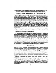
0.35 Projection errors True endmembers

Table 1. SRE(dB) in simulated data experiments. Library size 240 (Full size)

0.3

0.25 Projection error

NCLS

40 (1/6 × full size)

7.95

16.09

10.45

19.04

9 (exact number)

20.90

30.58

240 (Full size)

7.51 λ = 0.01

14.39 λ = 0.001

40 (1/6 × full size)

11.15 λ = 0.01

18.60 λ = 0.001

20 (1/12 × full size)

13.09 λ = 0.005

21.31 λ = 0.001

9 (exact number)

21.01 λ = 0.005

30.68 λ = 0.001

0.15

SUnSAL 0.05

0

50

100 150 Endmembers

200

250

Fig. 1. Projection errors in simulated data (SNR=30dB).

a number of spectra equal to the one estimated by HySime, we give a measure of the distance between the estimated subspace underlying the data and the new subspace defined by the retained members. We will call this measure “subspace error” and assume that it represents the Euclidean norm of the vector collecting the projection errors of the selected spectra. We should mention that, in our experiments, HySime identified the correct number of endmembers (nine) for both noise levels. Moreover, after applying the pruning methodology for the exact number of endmembers, we obtained exactly the set of signatures used to generate the data. This is already a very interesting indicator of the performance, as the spectral library used in the experiments contains, for each endmember, various spectrally similar signatures which might have been identified as endmembers instead of the true ones. For illustrative purposes, we plot in Fig. 1 the projection errors obtained for the library members when SNR=30dB. The true endmember signatures are highlighted with red circles. Note the very small projection errors correponding to these materials. Table 1 shows the SRE(dB) achieved by the two algorithms in all simulated instances, while Table 2 shows the processing times needed by each of them to solve the problem when SNR=30dB (full image considered). From both tables, it can be seen that the dictionary pruning methodology that we proposed not only improves considerably the accuracy of the unmixing results (see Table 1), but also leads to a significant decrease in the processing times (see Table 2). Finally the subspace errors for the two considered noise levels were: 0.411 for noise with SNR=30dB and 0.412 for SNR=40dB. The method identified correctly the data subspace in both cases, as only the true endmembers were retained from the library, but mismatches arise from the inexact estimation of the subspace in noisy data. Although the results obtained by the proposed method in simulated environments are encouraging, further experiments with real data sets are necessary. These will be conducted in the next section.

Table 2. Processing times [seconds] in simulated data affected by noise with SNR=30dB. Number of endmembers NCLS SUnSAL

240 52.45 23.57

40 4.57 2.64

20 2.09 1.98

9 0.65 0.62

4. EXPERIMENTS WITH REAL DATA The scene used in our real data experiments is the wellknown AVIRIS Cuprite data set, available online in reflectance units2 . The portion used in experiments corresponds to a 250 × 191-pixel subset of the sector labeled as f970619t01p02 r02 sc03.a.rfl in the online data. The scene comprises 224 spectral bands between 0.4 and 2.5 µm, with nominal spectral resolution of 10 nm. Prior to the analysis, bands 1–2, 105–115, 150–170, and 223–224 were removed due to water absorption and low SNR in those bands, leaving a total of 188 spectral bands. The Cuprite site is well understood mineralogically, and has several exposed minerals of interest, all included in the USGS library considered in experiments, denoted splib063 and released in September 2007. In our experiments, we use 302 spectra obtained from 2 http://aviris.jpl.nasa.gov/html/aviris.freedata.html 3 http://speclab.cr.usgs.gov/spectral.lib06

0.2 Projection errors 0.18 0.16 0.14 Projection error

0

SNR(dB)=40 12.19

20 (1/12 × full size)

0.2

0.1

SNR(dB)=30 5.18

0.12 0.1 0.08 0.06 0.04 0.02 0

0

50

100

150 Endmembers

200

250

Fig. 2. Projection errors in real data.

300

Alunite

Alunite: 924 pixels

0.45 0.4 50 0.35 0.3 100 0.25 0.2

150

0.15 0.1

200

0.05 250

0

50

100

150

0

Buddingtonite

Buddingtonite: 36 pixels 0.4 0.35

50

0.3 100

0.25 0.2

150 0.15 0.1

200

0.05 250

0

50

100

150

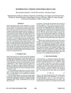
Given this mismatch due to calibration issues we did not retain the exact number of endmembers (18), but a larger one (40), to ensure the presence in the retained dictionary of all the endmember signatures. Fig. 3 shows a qualitative comparison between the reference classification maps extracted from the USGS map and the abundance fractions infered by SUnSAL after building a library composed of 40 members, using the methodology described in section 2.1. The parameter λ was set empirically to 0.001. Note the distribution of the materials of interest, which follows closely the reference maps. Also, the average running time per pixel was significantly reduced, from 2.6 milliseconds using the original library to 0.22 milliseconds using the pruned one (average over 20000 pixels and using the same computing environment, as in the simulated experiments).

Chalcedony

Chalcedony: 3262 pixels 0.35 50

0.3

5. CONCLUSIONS AND FUTURE WORK

0.25 100 0.2 150

0.15 0.1

200 0.05 250

0

50

100

150

0

Kaolinite

Kaolinite: 7424 pixels

0.6

0.5

50

0.4 100 0.3 150 0.2

In this paper, we have proposed a new methodology for dictionary pruning in sparse hyperspectral unmixing. Our experiments with simulated data show that the methodology leads to more accurate performances of the algorithms and reduces significantly the running time. Our experiments with real data show that unmixing methods obtain good results with a dramatically reduced running time. Despite the encouraging results, additional experiments should be conducted to mitigate the calibration issues that might occur during the process.

200 0.1

250

0

50

100

150

0

Fig. 3. USGS reference maps and fractional abundance maps derived by the proposed method for the dominant endmembers in the real scene .

6. REFERENCES [1] D. Iordache, J. Bioucas-Dias, and A. Plaza, “Sparse unmixing of hyperspectral data,” IEEE Transactions on Geoscience and Remote Sensing, vol. 49, no. 6, pp. 2014–2039, 2011. [2] D. Iordache, “A sparse regression approach to hyperspectral unmixing,” Ph.D. dissertation, Instituto Superior Tcnico, TULisbon, Lisbon, Portugal, 2011. [3] S. Chen, D. Donoho, and M. Saunders, “Atomic decomposition by basis pursuit,” SIAM review, vol. 43, no. 1, pp. 129–159, 2001.

this library as input to the unmixing methods described in section 2.1. A USGS Tetracorder map is available for hyperspectral data collected in 1995, while the publicly available AVIRIS Cuprite data was collected in 1997. Therefore, a direct comparison between the 1995 USGS map and the 1997 AVIRIS data is not possible. However, the USGS map serves as a good indicator for qualitative assessment of the fractional abundance maps produced by the unmixing algorithms discussed in section 2.1. Fig. 2 shows the projection errors of the members included in the spectral library. In experiments, the subspace dimension inferred by HySime was 18. After inspecting the ground–truth signatures included in the USGS map, there are only a few dominant endmembers in the scene which are considered in our analysis. Previously, we ran a calibration preprocessing step similar to the one in [1]. Note that, even after pre-calibrating the data using the actual library, there is still a gap between the library members and the data subspace.

[4] D. Iordache, J. Bioucas, and A. Plaza, “Total variation regularization in sparse hyperspectral unmixing,” Proc. 3rd IEEE GRSS Workshop on Hyperspectral Image and Signal Processing: Evolution in Remote Sensing (WHISPERS), Lisbon, Portugal, 2011. [5] D. Iordache, J. Bioucas-Dias, and A. Plaza, “Hyperspectral unmixing with Sparse Group Lasso,” IEEE International Geoscience and Remote Sensing Symposium IGARSS2011, Vancouver, Canada, 2011. [6] P. Sprechmann, I. Ramirez, G. Sapiro, and Y. Eldar, “C-hilasso: a collaborative hierarchical sparse modeling framework,” IEEE Transactions om Signal Processing, vol. 59, no. 9, pp. 4183–4198, September 2011. [7] J. Bioucas-Dias and M. Figueiredo, “Alternating direction algorithms for constrained sparse regression: application to hyperspectral unmixing,” 2nd Workshop on Hyperspectral Image and Signal Processing: Evolution in Remote Sensing (WHISPERS), 2010. [8] J. Nascimento and J. Bioucas-Dias, “Hyperspectral subspace identification,” IEEE Transactions on Geoscience and Remote Sensing, vol. 46, no. 10, pp. 2435–2445, 2008. [9] M. Zortea and A. Plaza, “Spatial preprocessing for endmember extraction,” IEEE Transactions on Geoscience and Remote Sensing, vol. 47, pp. 2679–2693, 2009.