Among the various applications of digital signal processing (DSP) is the generation of sound effects. These are needed in many instances such as in computer ...
1
Department of Computer Engineering College of Engineering Baghdad University
Digital Signal Processing and Sound Effects
Final-year project by:
Duaa Adil and Yazan Nehad
Submitted, May 2015
Supervised by:
Prof. Nuha A. S. Alwan
2
Abstract Among the various applications of digital signal processing (DSP) is the generation of sound effects. These are needed in many instances such as in computer games consoles, in tone generation for mobile cellular devices, and for theatrical performances, to name but a few. Generating high-quality sounds is of considerable import to the computer engineer when the latter is faced with the problem of dealing with fixed (usually small) memory budgets of computerized devices. The aim of this project is to explain and demonstrate the generation of sound effects via sound processing and sound synthesis. These two operations are fundamental applications of DSP and in particular digital filtering. Sound processing deals with the modification of sound (e.g. a prerecorded sound clip) using various types of digital filters and processors, whereas sound synthesis deals with the generation of certain application-specific sounds from scratch using math and software/ hardware implementation. All the above aspects of sound effects will be implemented and tested using the platform of the most commonly used technical computing software: MATLAB. It is hoped that the project will be of enough archival value to serve as a complementary and nonetheless often called-for back-up material for computer engineering students and specialists.
3
List of Abbreviations Abbreviation
Meaning
AM DFT DSP FFT FIR FT HPF
amplitude modulation discrete Fourier transform digital signal processing fast Fourier transform finite impulse response Fourier transform high-pass filter
IIR LPF PCM STFT
infinite impulse response low-pass filter pulse code modulation short-time Fourier transform
4
List of Figures Figure Captions
Page
Figure 2.1: Concert hall impulse response h(n). Figure 2.2: Production of tremolo in a sound signal by amplitude modulation (AM). Figure 3.1: The concept of sound synthesis. Figure 3.2: General network of candidate basic elements for sound synthesis techniques. Figure 3.3: Subtractive synthesis
13 14 17 17 18
5
Table of Contents Abstract ……………………….…………………………………………………..... 2 List of Abbreviations…...…………………….……………………………………... 3 List of Figures……………………………………………………………………….. 4 Table of Contents……………….………………………………………………….. . 5 Chapter One: Introduction …………….……………………………………………. 6 Chapter Two: Sound Processing ……………..…………………………………... . 10 Chapter Three: Sound Synthesis …………………………………………...…… ... 15 Chapter Four: Simulation Results………...……………………………………........19 Chapter Five: Conclusion and Future Prospects………………………………….....24 Appendix …………………………………………………………………………... 25 References ……………………………………………………………………….... 27
6
Chapter One Introduction 1.1 Overview Sound effects can be generated by digital signal processing (DSP) techniques, mainly digital filters. This involves either sound processing or sound synthesis. Sound processing makes use of one or a small number of prerecorded sound clips that undergo one or more stages of modification through processing or filtering to generate new modified sounds with desirable effects for certain applications. As for sound synthesis, the main sound synthesis method that will be dealt with in this study is the synthesis of impact sounds that help simulate realism in video games. For example, the user (player) may knock things over or throw objects around and therefore needs realistic audio to correspond to the animation. Sound synthesis is an attractive solution to the memory problem. Instead of storing multiple sound clips, they can be generated using math and software with minimum hardware requirements. Some sound effects such as the generation of echoes and reverberations require only linear digital filtering or processing. Linearity ensures that the frequency content of the processor input is transferred to the output though with different amplitude and phase. Other sound effects such as tremolo, however, require non-linear processors such as those producing modulation. In the latter case, new frequencies that are not present at the input are introduced at the processor output.
7
1.2 Digital filters:
These are classified into two major categories according to their impulse response: finite impulse response (FIR) and infinite impulse response (IIR). As their names indicate, FIR filters have a finite number of nonzero samples in their impulse responses, whereas IIR filters have impulse responses with an infinite number of samples. The advantages of IIR filters is that they can usually be implemented with lower order (thereby using fewer delay elements, fewer multipliers and less computation in software implementations) for the same performance as FIR filters. Moreover, they are easier to design to match a desired response. On the other hand, linear phase cannot be achieved with IIR filters and quantization effects are more serious due to feedback and for the same reason, they have stability problems [1].
1.3 Sound:
Sounds are time-varying signals in the real world and, indeed, all of the meaning is related to such time variability. Therefore, it is interesting to develop sound analysis techniques that allow to grasp at least some of the distinguished features of time-varying sounds, in order to ease the tasks of modification and re-synthesis [2].
8
1.3.1 Sound intensity:
The human ear is usually described as composed of three parts: the outer ear, the middle ear and the inner ear. Consider a sinusoidal source of sound in free space. It generates spherical pressure waves that carry energy. The acoustic intensity is the power by unit surface that is carried by a wave front. At 1000 Hz, the human ear can detect sound intensities ranging from 10-12 W/m2 to 1 W/m2 (the pain threshold) [2].
1.3.2 Sound Pitch
Periodic tones elicit a sensation of pitch, thus meaning that they can be ordered on a scale from low to high. Pitch is the sensorial correlate of frequency [2]. A high-pitch sound contains high frequencies and vice versa. As an illustrative example, a feminine human voice is considered high-pitch and a masculine voice is low-pitch.
1.3.3 Sound Analysis Any time-domain signal can be completely characterized by its frequency content or, in other words, its frequency-domain properties. Since sounds are time-varying signals, they cannot be described by simple Fourier analysis, but rather by the short-time Fourier transform (STFT). This is nothing more than the Fourier transform (FT) performed on slices of the time-domain signal. This is done to account for the time-varying nature of sound. Sound analysis is an essential necessity for the reverse process, namely sound synthesis. To synthesize certain sounds, one needs to
9
analyze a sound clip into the constituent frequency components in order to be able to synthesize similar and modified versions of this sound clip.
1.3.4 Tools for Sound Processing
Since the bases of sound signal processing are mathematics and computational science, it is recommended to use a technical computing software package for sound processing such as MATLAB [3]. Later, when sound applications are to be marketed, it is likely that the software algorithms analyzed and tested in MATLAB will be implemented on lowcost hardware specifically tailored for signal processing applications. In the MATLAB environment, the acquisition and writing of sound files from and to the disk is done by means of the functions 'wavread' and 'wavwrite' respectively. These two functions are detailed in the appendix as regards their syntax and description. Since sounds are handled as mono-dimensional vectors, sound processing can be entirely made up of vectorial operations. In contrast, the iterative sample-by-sample processing is quite inefficient with MATLAB which is designed to handle matrices. The rest of the project report is organized as follows: Chapter 2 and Chapter 3 deal with sound processing and sound synthesis respectively. Simulation results of various sound effects generation are illustrated in Chapter 4, accompanied by the corresponding MATLAB code. Finally, the conclusion and future prospects are given in Chapter 5.
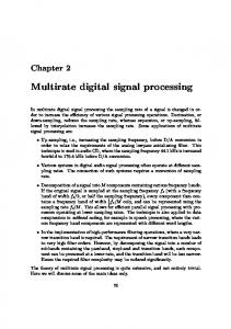
11
Chapter Two Sound processing
2.1 Overview Sound processing is the act of manipulating sounds and making them more interesting for a wide range of applications. Audio effects can be classified according to the way they process sound. Table 1 below shows different DSP techniques with the pertinent sound effects alongside.
Table 1: DSP techniques and the possible resulting sound effects DSP technique Basic filtering: LPF, HPF, BPF
Sound effect Noise removal and sound feature extraction
Equalizers
Bass and treble effects
Time-varying filtering
Wah-wah effect
Delays
Echoes and reverberations
Modulators
Tremolo
Non-linear processing
Distortions, exciters, limiters
Basic filtering accentuates certain frequency bands and attenuates others. This is mainly frequency-selective filtering aiming at noise removal or extraction of certain features such as pitch. This DSP operation is
11
somewhat restrictive compared to other DSP techniques that generate more interesting sound effects. Equalizers, on the other hand, amplify or diminish certain bands while leaving the others unchanged. This leads to certain desired sound effects such as bass and treble. Time varying filters such as variable-center-frequency BPFs produce the so-called wah-wah effect. These are used in electric guitars to produce a human-like sound mimicking the verbal 'wah-wah' sound. Delays can produce echoes and reverberations that are desirable in concerts and theatrical assembly halls. These sound effects are mainly produced by IIR and sometimes FIR digital filters. Modulators generate the tremolo effect that specifically results from amplitude modulation. However, the carrier here is the sound signal and the baseband signal is a very low-frequency sinusoidal signal. Non-linear processing such as limiters, compressors and expanders are used to control high sound peaks or boost low signal levels to create more lively sound characteristics.
In this project we will study: 1 – Effect of changing the pitch. 2 – Echo effect. 3 – Tremolo effect.
12
2.2 Effect of changing the pitch As we have mentioned, pitch is the sensorial correlate of frequency. Increasing the sampling frequency of a digital sound clip increases the pitch of the heard sound and vice versa. The MATLAB functions 'wavread' and 'wavwrite' (in the appendix) accommodate the possibility of changing the sample rate (fs) in Hertz.
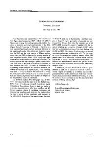
2.3 Echo Effect Echo — implies a distinct, delayed version of a sound, e.g. as you would hear with a delay more than one or two-tenths of a second (up to seconds). A piece of music played in a concert hall does not sound the same if played in a living room. This is due to the echoes (early reflections) and the reverberations (late reflections) that are different in different listening places. However, we can simulate a concert hall in a living room using one of the following DSP methods: A. Convolution and DFTs 1. Design a desired concert hall impulse response by placing several digital impulses a number of samples apart and with exponential decay or generally decreasing strengths. The impulse with the greatest strength is usually placed at the origin and represents the original sound. The other samples of the designed impulse response h(n), where n is the time index, are responsible for echoes. See Figure 2.1. 2. Take the FFT of h(n) to obtain the desired system frequency domain representation H(k), where k is the frequency index. 3. Take the FFT of the sound clip. Call it S(k).
13
4. Multiply H(k) by S(k) and take the inverse FFT of the product to produce output sound clip which contains the designed echoes and reverberations. This is naturally due to the fact that multiplication in the frequency domain is equivalent to the convolution in the time domain of the designed impulse response with the original sound clip sequence.
Figure 2.1: Concert hall impulse response h(n).
B. FIR and IIR digital filters
We wish to generate a single echo together with the original sound using
an
FIR
filter,
then
multiple
diminishing
echoes
(reverberations) using an IIR filter. 1. For echoes: y(n) = x(n) +α.x(n − N) , hence, H(z) = 1+α.z-N . This is an FIR filter. 2. For reverberations: s(n) = x(n) + β .s(n − M) , hence, H(z) = 1/(1− β .z-M ) . This is an IIR filter with M poles.
14
Method B will be used in this work. If Method A were to be implemented, we would need to zero-pad the impulse response and the original sound clip such that both are of the same length and that this length is enough to accommodate the number of samples that linear convolution would result in.
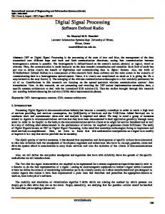
2.4. Tremolo Effect This effect involves the periodic modification of the sound intensity by a very low-frequency sinusoidal signal (single tone). This may be achieved by amplitude-modulating the sound signal by the low-frequency single tone to produce a trembling-like sound, hence the name 'tremolo'. This is demonstrated by Figure 2.2 where, as a special case, the sound is pictured as a higher-frequency single tone itself, which is obviously not always the case.
Figure 2.2: Production of tremolo in a sound signal by amplitude modulation (AM).
15
Chapter Three Sound Synthesis
3.1 Overview Sound synthesis deals with generating sounds from scratch using math and software/hardware implementation. This aspect has various applications
such
as
generating
electronic
music,
interactive
performances in computer games, the generation of ring and alert tones for mobile cellular devices, etc. The synthesis of impact sounds is of particular interest. We present a model for impact sound synthesis based on the response of different materials when they are struck. When a metal is struck, it rings. However, when wood is struck it just produces a thudding sound. For impact sound synthesis to succeed, it must be based on the converse, that is, sound analysis. Analyzing sounds is simply taking their spectrum to find the constituent frequencies. Then it is possible to generate different sounds by modifying amplitude, phase and frequency of the corresponding trigonometric components. The advantage of impact sound synthesis becomes manifest upon considering the limited audio memory budgets of gaming consoles for instance. Pre-recorded clips provide high quality and do not require computation, but they need to reside in memory because the latency of streaming from disk is too high. Therefore, sound synthesis emerges as an attractive solution to the sound problem [4].
16
3.2. Model for sound synthesis The model for sound synthesis can be described by the following equation which combines the different variables that can be adjusted to produce different impact sounds. ( )
where
( )
∑
(
( )
)
( )
( ) is the possibly time-varying amplitude,
possibly time-varying frequency,
is the phase and
( ) is the is a constant,
all related to the m-th sinusoidal component, and finally ( ) is a noise component [4].
Am(t) : e - αt , α is a decay constant. x(t) will them be a sound of impact (when an object is struck
for
example). We say that we are using additive synthesis to generate the impact sound. Additive synthesis refers to a number of related synthesis techniques, all based on the idea that complex tones can be created by the summation or addition of simpler ones. It is possible to break up any complex sound into a number of simpler tones, usually in the form of sine waves (Fourier). In additive synthesis, we use this theory in reverse. Additive synthesis uses a combination of harmonics or partials to create the basic tone colors or 'timbres ' and in more sophisticated systems several of these timbres can be combined to make the overall sound [5]. The decay factor is important to produce a realistic naturally-ending sound, rather than an abrupt artificial stop of the impact action.
17
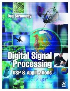
Figure 3.1: The concept of sound synthesis
To summarize, the main motivations of sound synthesis include [6]: 1. 2. 3. 4.
To reproduce existing sounds. To reproduce the physical process of sound generation. To generate new pleasant or useful sounds. To control/explore timbre.
Figure 3.2.: General network of candidate basic elements for sound synthesis techniques [6].
18
3.3 Subtractive Synthesis Is another linear technique based on the idea that sounds can be generated from subtracting (filtering out) components from a very rich signal (e.g. noise, square wave) as in Figure 3.3 [6].
Figure 3.3: Subtractive synthesis.
This idea is also depicted in Figure 3.2 which demonstrates a collection of candidate basic elements for sound synthesis. Not all blocks in Figure 3.2 are mandatory in sound synthesis. For example, for the impact sound synthesis described in Section 3.2, the vibrato input is not needed.
19
Chapter Four MATLAB code for sound effects and results The MATLAB functions "wavread" and "wavwrite" are employed for acquisition and writing of sound files respectively. They are described in detail in the appendix.
4.1. Changing the pitch: By using prerecorded sound clip ' Ohno' that consists of the utterance "Oh, no!". Code A: clc; clear all; close all; x=wavread('Ohno'); N=length(x); fs=45000; wavwrite(x,fs,'pitcheffect1')
Code B: clc; clear all; close all; x=wavread('Ohno'); N=length(x); fs=15000; wavwrite(x,fs,'pitcheffect2')
21
As is clear from the above codes, increasing the sampling frequency of a digital sound clip increases the pitch of the heard sound and vice versa. So we get many sound clips with each one having a different level of pitch by changing the sampling frequency (fs) as shown in the code. Normally, fs=22000 Hz for the original "Ohno" sound clip. When fs=15000 Hz (code B), the output it seem approximate a masculine human voice, but when fs=45000 Hz (code A), the output seems to approximate a feminine human voice.
4.2. The Echo Effect Also using the same pre-recorded sound clip when experimenting with sound pitch, we write and run the following code for demonstrating the echo effect: clc; close all; clear all; fs=22000; x=wavread('Ohno'); N=length(x); AA=zeros(1,N); g=[x' AA]; a1=0.4;a2=0.7; A=zeros(1,ceil(N/2)); B=1; k1=ceil(0.2*N); A(k1)=a1; k2=ceil(0.4*N); A(k2)=a2; y=filter(A,B,g); y1=g+y; wavwrite(y1,fs,'echoeffect');
Echo: is the multiple repetition of sound due to reasons such as reflection, etc.
21
Running the code enables us to hear the original "Ohno" utterance plus two echoes with different timing as programmed. Diagram of an echo-producing FIR filter (the main idea of the previous code):
X: the input Y: the output
4.3. Tremolo Effect clear all; clc ; close all; fs=22000; x=wavread('Ohno'); index=1:length(x); fc=20; alpha=0.5; trem=(1+alpha*sin(2*pi*index.*(fc/fs))); y=trem'.*x; wavwrite(y,fs,'tremoloeffect')
Tremolo: is the variation of the amplitude of the sound signal by a very low-frequency tone. Amplitude-modulating the sound signal or baseband signal by a lowfrequency tone or carrier (as can be deduced from the code) results in the
22
same sound signal but with a sinusoidally and slowly fluctuating envelope. This results in turn in a trembling sound effect of the utterance 'Ohno'. Y(t)=[1+alpha*x(t)]*carrier.
4.4. Impact Sounds clear all; clc; close all; t=0:0.01:100; aa=0.9995.^(t* 100); a=0.95.^(t*100); x1=a.*0.5.*cos(2*pi*t/0.1+(pi/8)); %x1=aa.*0.5.*cos(2*pi*t/0.9+(pi/8)); x2=aa.*0.2.*cos(2*pi*t/0.5); for i=1:10001; y(i)=0.05.*rand(1); end; y=aa.*y; x=x1+y; wavwrite(x,22000,'impactsound');
Sound synthesis: generating sounds starting from scratch using math and programming.
( )
∑
( )
(
( )
Am(t) : e - αt , α is a decay constant.
)
( )
23
The code uses two tones with two different frequencies as well as different exponential decay rates. When the two tones are of frequencies 10 Hz and 2 Hz, the impact sound very much resembles the natural sound produced upon gently striking a glass object with metal. When the two tones are 2 Hz and 1 Hz, the synthesized impact sound is very much that of the result of striking a sand bag, which is a thudding sound. In both cases the sounds end very naturally due to the exponentially decaying envelope.
24
Chapter Five Conclusion and Future Prospects We have discussed and simulated several sound processing methods to produce sound effects for a variety of applications. We have investigated the effect of changing the pitch, producing echoes and reverberations, and finally the tremolo effect. Digital filtering played an important role in the afore-mentioned methods of sound processing. We have also presented a mathematical model for synthesizing realistic impact sound. Modal synthesis of impact sounds enables us to save memory on gaming consoles. As a whole, the project revolves around familiarizing computer engineering students with facets of technological trends that undergo essential interaction with computer applications. The present work holds intriguing prospects for future investigation into the generation of impact sounds using digital filters. For example, simple filters can be developed to attenuate random portions of the frequency spectrum which can apply variations of impact sounds that are not possible with only modal synthesis. In this case, the digital filter is complementary to, and not a substitute for, modal synthesis.
25
Appendix
MATLAB functions for acquisition and writing of sound files [7]: waveread Y=wavread(FILE) reads a WAVE file specified by the string FILE,returning the sampled data in Y. The ".wav" extension is appended if no extension is given.
[Y,FS,NBITS]=wavread(FILE) returns the sample rate (FS) in Hertz and the number of bits per sample (NBITS) used to encode the data in the file.
[...]=wavread(FILE,N) returns only the first N samples from each channel in the file. [...]=wavread(FILE,[N1 N2]) returns only samples N1 through N2 from each channel in the file.
[Y,...]=wavread(...,FMT) specifies the data type format of Y used to represent samples read from the file. If FMT='double', samples.
Y
contains
double-precision
normalized
If FMT='native', Y contains samples in the native data type found in the file. Interpretation of FMT is case-insensitive, and partial matching is supported. If omitted, FMT='double'.
Output Scaling The range of values in Y depends on the data format FMT specified. Some examples of output scaling based on typical bit-widths found in a WAV file are given below for both 'double' and 'native' formats.
FMT='native' #Bits
MATLAB data type
-----
------------------------- -------------------
8
uint8
(unsigned integer)
Data range
0