Digital Signal Processing: Course Review

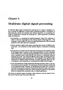
Course Review References:

Digital Signal Processing: Course Review

Sections: 1.1, 1.2, 1.3, 1.4 2.1, 2.2, 2.3, 2.4, 2.5 3.1, 3.2, 3.3, 3.4 4.1, 4.2, 4.3, 4.4, 5.1, 5.2, 5.4, 5.5 7.1, 7.2, 8.1 11.2, 11.3, 11.4 of John G. Proakis and Dimitris G. Manolakis, Digital Signal Processing: Principles, Algorithms, and Applications, 4th edition, 2007,

Professor Deepa Kundur University of Toronto

and supplementary audio, image and video processing notes.

Professor Deepa Kundur (University of Toronto)Digital Signal Processing: Course Review

1 / 97


2 / 97

Sampling Theorem If the highest frequency contained in an analog signal xa (t) is Fmax = B and the signal is sampled at a rate Fs > 2Fmax = 2B

Chapter 1: Introduction

then xa (t) can be exactly recovered from its sample values using the interpolation function g (t) =

sin(2πBt) 2πBt

Note: FN = 2B = 2Fmax is called the Nyquist rate.


3 / 97


4 / 97

Sampling Theorem

Bandlimited Interpolation

Sampling Period = T =

1 1 = Fs Sampling Frequency

Therefore, given the interpolation relation, xa (t) can be written as xa (t) =

x(n) samples

bandlimited interpolation function -- sinc

∞ X

xa (nT )g (t − nT )

n

n=−∞ 0

xa (t) =

∞ X

x(n) g (t − nT )

n=−∞

where xa (nT ) = x(n); called bandlimited interpolation.


5 / 97


Digital-to-Analog Conversion original/bandlimited interpolated signal

Digital-to-Analog Conversion

x(n)

original/bandlimited interpolated signal

1

n

0

I

I

Common interpolation approaches: bandlimited interpolation, zero-order hold, linear interpolation, higher-order interpolation techniques, e.g., using splines In practice, “cheap” interpolation along with a smoothing filter is employed.


6 / 97

7 / 97

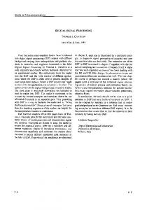
zero-order hold I

I

1

-3T -2T -T

0

T

2T

t

3T



8 / 97

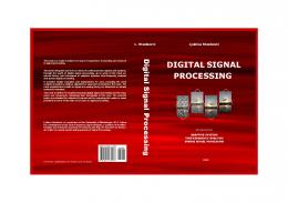
Digital-to-Analog Conversion original/bandlimited interpolated signal

-3T -2T -T

I

I

linear interpolation

1

0

T

2T

t

3T

Chapter 2: Discrete-Time Signals and Systems



9 / 97

Terminology: Input-Output Description


10 / 97

Classification of Discrete-Time Systems Common System Properties:

input/ excitation

x(n)

Discrete-time System

I

output/ response

Discrete-time signal

Discrete-time signal

I

y(n)

Input-output description (exact structure of system is unknown or ignored): y (n) = T [x(n)] “black box” representation:

vs.

dynamic

time-invariant

vs.

time-variant

linear

vs.

nonlinear

causal

vs.

non-causal

stable

vs.

unstable systems

.. .

T

x(n) −→ y (n) Professor Deepa Kundur (University of Toronto)Digital Signal Processing: Course Review

static

11 / 97

.. .


12 / 97

The Convolution Sum

The Convolution Sum

Let the response of a linear time-invariant (LTI) system to the unit sample input δ(n) be h(n). Therefore,

T

δ(n) −→ h(n) T

δ(n − k) −→ h(n − k)

y (n) =

T

α δ(n − k) −→ α h(n − k)

∞ X

x(k)h(n − k) = x(n) ∗ h(n)

k=−∞

T

x(k) δ(n − k) −→ x(k) h(n − k) ∞ ∞ X X T x(k)δ(n − k) −→ x(k)h(n − k) k=−∞

for any LTI system.

k=−∞ T

x(n) −→ y (n)


13 / 97

Finite vs. Infinite Impulse Response


14 / 97

System Realization

Implementation: Two classes General expression for Nth-order LCCDE:

Finite impulse response (FIR): y (n) =

M−1 X

N X

) h(k)x(n − k)

nonrecursive systems

k=0

M X ak y (n−k) = bk x(n−k)

a0 , 1

k=0

k=0

Initial conditions: y (−1), y (−2), y (−3), . . . , y (−N). Infinite impulse response (IIR): y (n) =

∞ X

) h(k)x(n − k)

Need: (1) constant scale, (2) addition, (3) delay elements.

recursive systems

k=0


15 / 97


16 / 97

Building Block Elements

y (n) = −

+

N X

ak y (n − k) +

k=1

Constant multiplier:

+


17 / 97

Direct Form I IIR Filter Implementation

M X


18 / 97

Direct Form II IIR Filter Implementation

+

+

+

+

+

+

+

+

+

+

+

LTI All-zero system

+

+

LTI All-pole system

LTI All-pole system

Requires: M + N + 1 multiplications, M + N additions, M + N memory locations Professor Deepa Kundur (University of Toronto)Digital Signal Processing: Course Review

...

+

...

+

...

+

...

+

...

+

...

...

v(n)

k=0

bk x(n − k) nonrecursive | {z } k=0 input 1 N X y (n) = − ak y (n − k) + v (n) recursive |{z} |{z} k=1 output 2 input 2 v (n) = |{z} output 1

Unit advance:

+

bk x(n − k)

is equivalent to the cascade of the following systems:

Unit delay:

Signal multiplier:

M X

...

Adder:

Direct Form I vs. Direct Form II Realizations

19 / 97

+

LTI All-zero system

Requires: M + N + 1 multiplications, M + N additions, M + N memory locations Professor Deepa Kundur (University of Toronto)Digital Signal Processing: Course Review

20 / 97

Direct Form II IIR Filter Implementation +

+

+

+

+

+

Chapter 3: The z-Transform and Its Applications

...

...

+

...

+

+

...

+

For N>M

Requires: M + N + 1 multiplications, M + N additions, max(M, N) memory locations Professor Deepa Kundur (University of Toronto)Digital Signal Processing: Course Review

Adder:

22 / 97

Region of Convergence

Unit delay:

Constant multiplier: Direct z-Transform: ∞Unit advance: X X (z) = x(n)z −n

I

the region of convergence (ROC) of X (z) is the set of all values of z for which X (z) attains a finite value

I

The z-Transform is, therefore, uniquely characterized by:

n=−∞ +

Signal multiplier: I


+

The Direct z-Transform I

21 / 97

Notation: X (z)

≡

1. expression for X (z) 2. ROC of X (z)

Z{x(n)}

Z

x(n) ←→ X (z)


23 / 97


24 / 97

ROC Families: Finite Duration Signals


ROC Families: Infinite Duration Signals

25 / 97

z-Transform Properties Property Notation:


26 / 97

Convolution using the z-Transform

Linearity: Time shifting:

Time Domain x(n) x1 (n) x2 (n) a1 x1 (n) + a2 x2 (n) x(n − k)

z-Domain X (z) X1 (z) X2 (z) a1 X1 (z) + a2 X2 (z) z −k X (z)

z-Scaling: Time reversal Conjugation: z-Differentiation: Convolution:

an x(n) x(−n) x ∗ (n) n x(n) x1 (n) ∗ x2 (n)

X (a−1 z) X (z −1 ) X ∗ (z ∗ ) dX (z) −z dz X1 (z)X2 (z)

Basic Steps: 1. Compute z-Transform of each of the signals to convolve (time domain → z-domain):

ROC ROC: r2 < |z| < r1 ROC1 ROC2 At least ROC1 ∩ ROC2 At least ROC, except z = 0 (if k > 0) and z = ∞ (if k < 0) |a|r2 < |z| < |a|r1 1 < |z| < r1 r1 2 ROC r2 < |z| < r1 At least ROC1 ∩ ROC2

X1 (z) = Z{x1 (n)} X2 (z) = Z{x2 (n)} 2. Multiply the two z-Transforms (in z-domain): X (z) = X1 (z)X2 (z) 3. Find the inverse z-Transformof the product (z-domain → time domain): x(n) = Z −1 {X (z)}

among others . . .


27 / 97


28 / 97

Common Transform Pairs 1 2 3 4 5 6

Signal, x(n) δ(n) u(n) an u(n) nan u(n) −an u(−n − 1) −nan u(−n − 1)

7

cos(ω0 n)u(n)

8

sin(ω0 n)u(n)

9

an

10

an

cos(ω0 n)u(n) sin(ω0 n)u(n)

z-Transform, X (z) 1 1 1−z −1 1 1−az −1 az −1 (1−az −1 )2 1 1−az −1 az −1 (1−az −1 )2 1−z −1 cos ω0 1−2z −1 cos ω0 +z −2 z −1 sin ω0 1−2z −1 cos ω0 +z −2 1−az −1 cos ω0 1−2az −1 cos ω0 +a2 z −2 1−az −1 sin ω0 1−2az −1 cos ω0 +a2 z −2

Common Transform Pairs ROC All z |z| > 1 |z| > |a| |z| > |a| |z| < |a| |z| < |a|

1 2 3 4 5 6

Signal, x(n) δ(n) u(n) an u(n) nan u(n) −an u(−n − 1) −nan u(−n − 1)

|z| > 1

7

cos(ω0 n)u(n)

|z| > 1

8 9

cos(ω0 n)u(n)

10

an

sin(ω0 n)u(n)

|z| > |a| |z| > |a|


29 / 97

Common Transform Pairs

sin(ω0 n)u(n) an

z-Transform, X (z) 1 1 1−z −1 1 1−az −1 az −1 (1−az −1 )2 1 1−az −1 az −1 (1−az −1 )2 1−z −1 cos ω0 1−2z −1 cos ω0 +z −2 z −1 sin ω0 1−2z −1 cos ω0 +z −2 1−az −1 cos ω0 1−2az −1 cos ω0 +a2 z −2 1−az −1 sin ω0 1−2az −1 cos ω0 +a2 z −2

ROC All z |z| > 1 |z| > |a| |z| > |a| |z| < |a| |z| < |a| |z| > 1 |z| > 1 |z| > |a| |z| > |a|


30 / 97

The System Function Z

h(n) ←→ H(z) I

z-Transform expressions that are a fraction of polynomials in z −1 (or z) are called rational.

Z

time-domain ←→ z-domain Z impulse response ←→ system function Z

y (n) = x(n) ∗ h(n) ←→ Y (z) = X (z) · H(z) I

z-Transforms that are rational represent an important class of signals and systems. Therefore, H(z) =


31 / 97

Y (z) X (z)


32 / 97

The System Function of LCCDEs

y (n) = −

N X

ak y (n − k) +

k=1

Z{y (n)} = Z{−

M X

ak y (n − k) +

M X

k=1

Z{y (n)} = − Y (z) = −

k=1 N X

bk x(n − k)

Y (z) +

k=0

N X

N X

The System Function of LCCDEs

"

bk x(n − k)}

ak Z{y (n − k)} +

Y (z) 1 +

k=1

=

bk Z{x(n − k)}

M X

bk z −k X (z)

k=0 N X

# ak z −k

=

k=1

X (z)

M X

bk z −k

k=0

H(z) =

k=0

ak z −k Y (z) +

ak z −k Y (z)

k=1

k=0 M X

M X

N X

Y (z) X (z)

PM

=

−k k=0 bk z h i P 1 + Nk=1 ak z −k

LCCDE ←→ Rational System Function

bk z −k X (z)

k=0

Many signals of practical interest have a rational z-Transform.


33 / 97


34 / 97

Inversion of the z-Transform Three popular methods: 1. Contour integration: I 1 x(n) = X (z)z n−1 dz 2πj C

Chapter 4: Frequency Analysis of Signals

−1

2. Expansion into a power series in z or z : ∞ X X (z) = x(k)z −k k=−∞

and obtaining x(k) for all k by inspection. 3. Partial-fraction expansion and table look-up.


35 / 97


36 / 97

CTFT: Intuition

CTFT: Duality

1 x(t) = 2π

Z

∞

X (Ω)e jΩt dΩ

Z ∞ 1 x(t) = X (Ω)e jΩt dΩ 2π −∞ Z ∞ X (Ω) = x(t)e −jΩt dt

−∞

I

We may consider x(t) as a linear combination of e jΩt for Ω ∈ R.

I

The larger |X (Ω)|, the more x(t) will look like a sinusoid with Ω.

−∞

F

Shape A ←→ Shape B F

Shape B ←→ Shape A F

Operation A ←→ Operation B F

Operation B ←→ Operation A


37 / 97

CTFT: Magnitude and Phase


Complex Sinusoids: Discrete-Time e jωn = cos(ωn) + j sin(ωn)

≡

dst-time complex sinusoid

cos(2πfn)

∞ 1 X (Ω)e jΩt dΩ 2π −∞ Z ∞ 1 = |X (Ω)|e j∠X (Ω) e jΩt dΩ 2π −∞ Z ∞ = |X (Ω)|e j(Ωt+∠X (Ω)) df

Z

x(t)

38 / 97

=

n

∞ 0

I

|X (Ω)| dictates the relative presence of the sinusoid of frequency Ω in x(t).

I

∠X (Ω) dictates the relative alignment of the sinusoid of frequency Ω in x(t).

sin(2πfn)

n

0


39 / 97


40 / 97

Classification of Fourier Pairs

Duality PER

PERIODIC

APERIODIC

CTS-TIME Continuous-Time Fourier Series (CTFS) Continuous-Time Fourier Transform (CTFT)

DST-TIME Discrete-Time Fourier Series (DTFS) Discrete-Time Fourier Transform (DTFT)

APER

CTS-TIME P j2πkF0 t x(t) = ∞ k=−∞ ck e R ck = T1p Tp x(t)e −j2πkF0 t dt R∞ 1 jΩt dΩ x(t) = 2π −∞ X (Ω)e R∞ −jΩt X (Ω) = −∞ x(t)e dt

DST-TIME P j2πkn/N x(n) = N−1 k=0 ck e P N−1 ck = N1 n=0 x(n)e −j2πkn/N R 1 X (ω)e jωn dω x(n) = 2π P∞2π X (ω) = n=−∞ x(n)e −jωn

F

periodic ←→ discrete F

discrete ←→ periodic F

aperiodic ←→ continuous F

continuous ←→ aperiodic Professor Deepa Kundur (University of Toronto)Digital Signal Processing: Course Review

41 / 97

Discrete-Time Fourier Series (DTFS)


DTFS: Example Pair

For discrete-time periodic signals with period N: I

x(n) x(n) A A

Synthesis equation: x(n) =

N−1 X

ck e j2πkn/N

-N -N

k=0 I

42 / 97

Analysis equation:

-L -L

0 0

L L

N N

n n

cc k k

ck =

N−1 1 X x(n)e −j2πkn/N N n=0

c0 0

0 0

Convergence conditions: None due to finite sums. Professor Deepa Kundur (University of Toronto)Digital Signal Processing: Course Review

43 / 97


k k

44 / 97

Discrete-Time Fourier Transform (DTFT)

DTFT: Example Pair

For discrete-time aperiodic signals: I

1 x(n) = 2π I

x(n) x(n)

Synthesis equation: Z

A A

X (ω)e jωn dω

2π -L -L

Analysis equation: X (ω) =

∞ X

0 0

n n

L L

x(n)e −jωn

n=−∞

Convergence conditions: ∞ X

|x(n)| < ∞

0 0

n=−∞ Professor Deepa Kundur (University of Toronto)Digital Signal Processing: Course Review

45 / 97


46 / 97

DTFT Theorems and Properties ck

x(t)

CTFS

A

c0

sinc -5 -4 -3

t

3 -2 -1

0

1

2

4

5

k

Property Notation:

Linearity: Time shifting: Time reversal Convolution: Correlation:

Time Domain x(n) x1 (n) x2 (n) a1 x1 (n) + a2 x2 (n) x(n − k) x(−n) x1 (n) ∗ x2 (n) rx1 x2 (l) = x1 (l) ∗ x2 (−l)

Wiener-Khintchine:

rxx (l) = x(l) ∗ x(−l)

x(t)

CTFT

A

0

ck

x(n)

DTFS

A

-L

-N

0

X(0)

sinc

t

L

n

N

c0

0

k

Frequency Domain X (ω) X1 (ω) X1 (ω) a1 X1 (ω) + a2 X2 (ω) e −jωk X (ω) X (−ω) X1 (ω)X2 (ω) Sx1 x2 (ω) = X1 (ω)X2 (−ω) = X1 (ω)X2∗ (ω) [if x2 (n) real] Sxx (ω) = |X (ω)|2

x(n)

-L

0

L

among others . . .

DTFT

A n


0

47 / 97


48 / 97

DTFT Symmetry Properties Time Sequence x(n) x ∗ (n) x ∗ (−n) x(−n) xR (n) jxI (n)

x(n) real

xe0 (n) = 12 [x(n) + x ∗ (−n)] xo0 (n) = 21 [x(n) − x ∗ (−n)]

DTFT X (ω) X ∗ (−ω) X ∗ (ω) X (−ω) Xe (ω) = 12 [X (ω) + X ∗ (−ω)] Xo (ω) = 12 [X (ω) − X ∗ (−ω)] X (ω) = X ∗ (−ω) XR (ω) = XR (−ω) XI (ω) = −XI (−ω) |X (ω)| = |X (−ω)| ∠X (ω) = −∠X (−ω) XR (ω) jXI (ω)


Chapter 5: Frequency Domain Analysis of LTI Systems

49 / 97


50 / 97

LTI

Linear Time-Invariant LTI (LTI) Systems

Linear Time-Invariant (LTI) Systems

LTI LTI ??? real n

LTI

0

imaginary

LTI

n

LTI Professor Deepa Kundur (University of Toronto)Digital Signal Processing: Course Review

0

51 / 97


52 / 97

???

Linear Time-Invariant (LTI) Systems

Frequency Response of LTI Systems

LTI

z-Domain

ω-Domain z=e jω

real

H(z) =⇒ H(ω)

real

z=e jω

system function =⇒ frequency response n

n

0

z=e jω

0

imaginary

Y (z) = X (z)H(z) =⇒ Y (ω) = X (ω)H(ω)

imaginary n

n

0

0

imaginary imaginary Professor Deepa Kundur (University of Toronto)Digital Signal Processing: Course Review

53 / 97

complex plane complex plane

LTI


54 / 97

imaginary

complex plane

imaginary

real

complex plane

imaginary

real

complex plane

LTI Systems as Frequency-Selective Filters

real real

complex plane complex plane

complex plane complex plane complex plane complex plane

complex plane complex plane complex plane

imaginary imaginary

real

I

Filter: device that discriminates, according to some attribute of the input, what passes through it

I

For LTI systems, given Y (ω) = X (ω)H(ω)

real real

imaginary real imaginary imaginary imaginary

real real

I

real imaginary

H(ω) acts as a kind of weighting function or spectral shaping function of the different frequency components of the signal

real imaginary imaginary


LTI system ⇐⇒ Filter

real real

55 / 97


56 / 97

Ideal Filters

Invertibility of Systems Sharp Transition

Ideal Lowpass Filter

Passband

Stopband

Stopband

I

Invertible system: there is a one-to-one correspondence between its input and output signals

I

the one-to-one nature allows the process of reversing the transformation between input and output; suppose

0 Sharp Transition

Classification: I

lowpass

I

highpass

Passband

Stopband

bandpass

I

bandstop

I

all-pass

Ideal Highpass Filter

0

Sharp Transition Passband

I

Passband

Stopband

y (n) = T [x(n)] where T is one-to-one w (n) = T −1 [y (n)] = T −1 [T [x(n)]] = x(n)

Ideal Bandpass Filter

Passband

0

Passband

Passband Stopband

Passband

Identity System

Ideal Badstop Filter

Stopband

0

Inverse System

Direct System

Ideal All-pass Filter

Passband 0


57 / 97

Invertibility of LTI Systems


58 / 97

Invertibility of LTI Systems

Identity System I

Therefore, h(n) ∗ hI (n) = δ(n)

Direct System

Inverse System

I I

Impluse response = LTI

Direct System

LTI

H(z)HI (z) = 1 HI (z) =

Inverse System


For a given h(n), how do we find hI (n)? Consider the z−domain

59 / 97

1 H(z)


60 / 97

Invertibility of Rational LTI Systems I

Suppose, H(z) is rational: A(z) B(z) B(z) HI (z) = A(z) poles of H(z) = zeros of HI (z) zeros of H(z) = poles of HI (z)

Chapter 7: The Discrete Fourier Transform

H(z) =


61 / 97

Intuition


62 / 97

Intuition Example

aperiodic + dst in time

DTFT ←→

↓ periodic repetition periodic + dst in time

cts + periodic in freq

A

↓ sampling DTFS ←→

dst + periodic in freq 0123 4

-N

one period of dst-time samples n = 0, 1, . . . , N − 1

DFT ←→

N-1 N

...

n

DTFT

one period of dst-freq samples k = 0, 1, . . . , N − 1

Therefore, we define the Discrete Fourier Transform (DFT) as being a computable transform that approximates the DTFT.

0 ...


63 / 97


64 / 97

Intuition

Intuition

Example

Example

A

-N

0123 4

A

N-1 N

...

n

0123 4

-N

DTFT DTFS

N-1 N

n

DFT

4 -N

...

...

0 1 2 3

N-1 N

4

k

0 1 2 3

-N

N-1N

k

...


65 / 97

Intuition


66 / 97

DTFT, DTFS and DFT

Example DTFT

←→

x(n) for all n A

-N

0123 4

...

N-1 N

↓ periodic repetition ∞ X xp (n) = x(n + lN) for all n

n

xˆ(n) where

and 0 1 2 3

N-1N

k

DTFS

←→

X (k) = X (ω)|ω= 2π for all k N k

DFT

ˆ (k) X

ˆ (k) = X

←→

xp (n) 0

for n = 0, . . . , N − 1 otherwise

X (k) 0

for k = 0, . . . , N − 1 otherwise

xˆ(n) =

-N

↓ sampling

l=−∞

DFT

4

X (ω) for all ω

...


67 / 97


68 / 97

The Discrete Fourier Transform Pair

Frequency Domain Sampling I

I

DFT and inverse-DFT (IDFT): N−1 X

X (k) =

n

x(n)e −j2πk N ,

n=0 N−1 X

1 N

x(n) =

Recall, sampling in time results in a periodic repetition in frequency.

n

X (k)e j2πk N ,

←→

x(n) = xa (t)|t=nT

k = 0, 1, . . . , N − 1 I

n = 0, 1, . . . , N − 1

k=0

∞ 2π 1 X Xa (ω + X (ω) = k) T k=−∞ T

F

Similarly, sampling in frequency results in periodic repetition in time.

Note: we drop the ˆ· notation from now on.

xp (n) =

∞ X

F

←→

x(n + lN)

X (k) = X (ω)|ω= 2π k N

l=−∞


69 / 97


70 / 97

Frequency Domain Sampling and Reconstruction


N =4

N =4 l=-2

x (n)

x (n+2N)

2

-6

-5

-4

-3

-2

-1

0

1

2

3

4

5

6

n

7

-7

-6

-5

-4

-3

-2

l=1

l=0

+

+

-1

0

1

2

l=2

x (n-N)

x (n)

+

+

...

1

-7

l=-1

x (n+N)

3

4

5

6

l=-2

7

n

-5

-7

-6

-5

-4

-3

-2

-1

0

l=0

l=1

+

2

3

4

5

6

n

7

-7

x (n-2N) +

+ 1

l=2

x (n-N)

x (n)

+

...

1

+

-6

-5

-4

-3

-2

-1

2

3

4

5

6

7

0

1

2

3

4

5

6

7

n

overlap ~

x (n)

support length = 4 = N

-6

x (n+2N)

2

...

no overlap

-7

x (n)

x (n-2N)

l=-1

x (n+N)

-4

-3

-2

-1

0

x~ (n)

support length = 6 > N

2

2

1

1

1

2

3

4

5

6


= x (n)

7

n

-7

71 / 97

-6

-5

-4

-3

-2

-1

0

1


=x(n)

n 72 / 97


Important DFT Properties

N =4 x(n)

-7

-6

-5

-4

-3

-2

-1

xp(n)

no temporal aliasing

2

2

1

1

0

1

2

3

4

5

6

7

n

-7

-6

-5

-4

-3

-2

-1

0

1

2

3

4

5

6

7

n

4

5

6

7

n

=x(n) x(n)

-7

-6

-5

-4

-3

-2

-1

0

time-domain aliasing

xp(n)

2

2

1

1

1

2

3

4

5

6

7

n

-7

-6

-5

-4

-3

-2

-1

0

1

2

3

Property Notation: Periodicity: Linearity: Time reversal Circular time shift: Circular frequency shift: Complex conjugate: Circular convolution: Multiplication: Parseval’s theorem:

Time Domain x(n) x(n) = x(n + N) a1 x1 (n) + a2 x2 (n) x(N − n) x((n − l))N x(n)e j2πln/N x ∗ (n) x1 (n) ⊗ x2 (n) x1 (n)x2 (n) PN−1 ∗ n=0 x(n)y (n)

Frequency Domain X (k) X (k) = X (k + N) a1 X1 (k) + a2 X2 (k) X (N − k) X (k)e −j2πkl/N X ((k − l))N X ∗ (N − k) X1 (k)X2 (k) 1 X1 (k) ⊗ X2 (k) N P N−1 1 ∗ k=0 X (k)Y (k) N

=x(n) Professor Deepa Kundur (University of Toronto)Digital Signal Processing: Course Review

73 / 97


74 / 97

Radix-2 FFT

Chapter 8: The Fast Fourier Transform

Two strategies: I Decimation in time (our focus in the lecture) I Decimation in frequency

I


75 / 97

Note: We assume that N is a power of two; i.e., N = 2r .


76 / 97

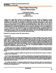
Radix-2 FFT: Decimation-in-time

Radix-2 FFT: Decimation-in-time

For N = 8.

For N = 8.

x(0) x(4) x(2) x(6)

Combine 2-point DFTs

2-point DFT

x(1) x(5)


2-point DFT

x(3) x(7)

Stage 1

x(0)

2-point DFT


2-point DFT

x(4)

X(0) X(1) X(2) X(3) X(4) X(5) X(6) X(7)

Stage 3

X(0) X(1)

-1 0 W8

x(2)

X(2)

-1 2

x(6)

W8 0

W8

-1

x(5)

0 W8

-1 1 W8 0

W8

-1

-1 0

W8 -1

2 W8 0

W8

-1

X(4) X(5)

2

W8

x(3)

77 / 97

X(3)

-1

x(1)

x(7)


0

W8

Stage 2

-1 3 W8

-1

-1

X(6) X(7)


78 / 97

FFT Complexity A = a + W Nr b

a r

b

I

I

A = a - W Nr b

Chapter 11: Multirate Digital Signal Processing

one complex multiplication two complex additions

In total, there are: I I

I

-1

Each butterfly requires: I

I

WN

N 2

butterflies per stage log N stages

Order of the overall DFT computation is: O(N log N).


79 / 97


80 / 97

Sampling Rate Conversion I

Sampling of Discrete-Time Signals Suppose a discrete-time signal x(n) is sampled by taking every Dth sample as follows:

Goal: Given a discrete-time signal x(n) sampled at period T from an underlying continuous-time signal xa (t), determine a new sequence xˆ(n) that is a sampled version of xa (t) at a different sampling rate Td . x(n) = xa (nT )

xd (n) = x(nD),

xˆ(n) = xa (nTd )

Decimation example: D = 2: x(n)

x(n)

-2

-1

0

1

2

-3

n

3

-2

0

-3

2

n

3

1

2


Td = 2T

-2

n

3 0

1

1

Td

1

-1

-1

xd (n)

x(n)

-2

T

1

T

1

-3

for all n

81 / 97

0

1

3

x (n)

Professor Deepa Kundur (University of Toronto)Digital Signal dProcessing: Course Review

1

-2

2

1/T ...

-1

0

1

2

n

3

1

...

F

0

Xd (F)

xd (n)

1/Td

Td = 2T ...

-2

n

2 -1

-3

0

1

3

1

...

F

0

Xd (F)

xd (n)

1/Td

Td = 4T ...

-1 -3

-2

3

X (F) T

1

-2

n

1 0

Decimation example: D = 2, 4:

x(n)

-3

82 / 97

Td = 4T

-1 -3

Decimation example: D = 2, 4:

n

2 -1

-3

1 0


2

3

n 83 / 97

... 0


F 84 / 97

Downsampling with Anti-Alaising Filter

−π/D ≤ ω ≤ π/D is expanded into −π ≤ ω ≤ π

Decimator LTI Filter

Downsampler

ANTI-ALIASED VERSION

X( ) 1/T

...

... 0

Xd ( ) 1/Td ...

The anti-aliasing filter Hd (ω) should have effective 1 continuous-time frequency cutoff of F0 = 2DT Hz, which is equivalent to a normalized cutoff of:

I

Interpolator

Upsampler

f0 =

LTI 1 Filter 1

F0 1 = · = Fs 2DT Fs 2D

LTI Filter

or

... 0

Xd ( )

Decimator 1Downsampler π

ω0 = 2π

2D

=

1/Td ...

D

... 0


85 / 97

86 / 97

Interpolation of Discrete-time Signals

−π/D ≤ ω ≤ π/D is expanded into −π ≤ ω ≤ π ANTI-ALIASED VERSION


X( )

...

To achieve this, consider a two-stage process: I Stage 1: Upsample to appropriately compress the spectrum. I Stage 2: Then filter with an appropriate lowpass filter.

... 0

I

We will consider upsampling by a factor of I . I

Xd ( ) ...

Note: we change here the interpolation factor from D to I to distinguish our results from decimation.

... 0


87 / 97


88 / 97

Interpolation by a Factor I

Interpolation of Discrete-time Signals

Interpolator LTI Filter

Upsampler

I

I

Upsampling (without filtering) can be represented as: x(m/I ) m = 0, ±I , ±2I , . . . v (m) = 0 otherwise V (ω) = X (ωI )

Interpolation only increases the visible resolution of the signal. No new information is gained. Interpolator LTI Filter

LTI Filter

Decimator Downsampler


89 / 97

Interpolation example: I = 4: upsampling + lowpass filtering


90 / 97

Interpolation example: I = 4: upsampling + lowpass filtering X( )

x(n) 1

... -1 -3

1

-2

2

0

3

n

... 0

V( )

v(n) 1

... -3

-2

-1

0

1

2

3

n

... 0

Y( )

y(n) 1

... -3

-2

-1

0

1

2

3


n 91 / 97

... 0


92 / 97

Sampling Rate Conversion by I /D

−π ≤ ω ≤ π is compressed into −π/I ≤ ω ≤ π/I

Interpolator

X( )

Upsampler

...

LTI Filter

LTI Filter


... 0

I I

x(n): original samples at sampling rate Fx y (n): new samples at sampling rate Fy

XI ( ) ...

... 0


93 / 97


94 / 97

Sampling Rate Conversion by I /D Interpolator Upsampler

LTI Filter

Upsampler

LTI Filter

LTI Filter


Downsampler

H(ω) = Hu (ω)Hd (ω) =


95 / 97

I 0 ≤ |ω| ≤ min(π/D, π/I ) 0 otherwise


96 / 97

Sampling Rate Conversion by I /D Interpolator Upsampler

LTI Filter

Upsampler

LTI Filter

I/D Rate Converter LTI Filter


Downsampler


97 / 97

Digital Signal Processing: Course Review

Digital Signal Processing: Course Review

Suggest Documents

Applied Digital Signal Processing

Digital Signal Processing

digital signal processing - fmcet

Advanced Digital Signal Processing

Digital Signal Processing

BIOMEDICAL DIGITAL SIGNAL PROCESSING

Digital Signal Processing

Digital Signal Processing

digital signal processing

for Digital Signal Processing

Digital Signal Processing

Digital Signal Processing

ELEC3104: Digital Signal Processing

Digital Signal Processing

Digital Signal Processing

Multirate digital signal processing

Digital Signal Processing

LabVIEW Signal Processing Course Manual

EE381K-8: Digital Signal Processing Fall 2013 Course Projects ...

Development of a Web-based Digital Signal Processing Course:

Download A Course in Digital Signal Processing Best ... - Google Sites

course syllabus: ee483 - introduction to digital signal processing

Syllabus ECE 512 – Digital Signal Processing – Fall 2013 Course ...

course syllabus: ee483 - introduction to digital signal processing