Direct minimization for calculating invariant subspaces in ... - CiteSeerX

arXiv:0805.1190v1 [math.NA] 8 May 2008

Direct minimization for calculating invariant subspaces in density functional computations of the electronic structure ∗ R. Schneider, T. Rohwedder, A. Neelov, J. Blauert

Abstract In this article, we analyse three related preconditioned steepest descent algorithms, which are partially popular in Hartree-Fock and Kohn-Sham theory as well as invariant subspace computations, from the viewpoint of minimization of the corresponding functionals, constrained by orthogonality conditions. We exploit the geometry of the of the admissible manifold, i.e. the invariance with respect to unitary transformations, to reformulate the problem on the Grassmann manifold as the admissible set. We then prove asymptotical linear convergence of the algorithms under the condition that the Hessian of the corresponding Lagrangian is elliptic on the tangent space of the Grassmann manifold at the minimizer.

1

Introduction

On the length-scale of atomistic or molecular systems, physics is governed by the laws of quantum mechanics. A reliable computation required in various fields in modern sciences and technology should therefore be based on the first principles of quantum mechanics, so that ab initio computation of the electronic wave function from the stationary electronic Schr¨odinger equation is a major working horse for many applications in this area. To reduce computational demands, the high dimensional problem of computing the wave function for N electrons is often, for example in Hartree-Fock and Kohn-Sham theory, replaced by a nonlinear system of equations for a set Φ = (ϕ1 , . . . , ϕN ) of single particle wave functions ϕi (x) ∈ V = H 1 (R3 ). This ansatz corresponds to the following abstract formulation for the minimization of a suitable energy functional J : ∗

This work was supported by the DFG SPP 1445: “Modern and universal first-principles methods for many-electron systems in chemistry and physics” and the EU NEST project BigDFT.

1

Problem 1: Minimize J : V N → R,

J (Φ) = J (ϕ1 , . . . , ϕN ) −→ min,

(1.1)

where J is a sufficiently often differentiable functional which is (i) invariant with respect to unitary transformations, i.e. N X J (Φ) = J (ΦU) = J (( ui,j φj )N i=1 ),

(1.2)

j=1

for any orthogonal matrix U ∈ Rn×n , and (ii) subordinated to the orthogonality constraints Z hϕi , ϕj i := ϕi (x)ϕj (x)dx = δi,j .

(1.3)

R3

In the present article, we shall be concerned with minimization techniques for J along the admissible manifold characterized by (1.3). The first step towards this will be to set up the theoretical framework of the Grassmann manifold to be introduced in section 2, reflecting the constraints (i) and (ii) imposed on the functional J and the minimizer Φ, respectively. In applications in electronic structure theory, formulation of the first order optimality (necessary) condition for the problem (1.1) results in a nonlinear eigenvalue problem of the kind: AΦ ϕi = λi ϕi ,

λ1 ≤ λ2 ≤ . . . ≤ λN

(1.4)

for N eigenvalues λi and the corresponding solution functions assembled in Φ. In these equations, the operator AΦ , is a symmetric bounded linear mapping AΦ : V = H 1 (R3 ) → V 0 = H −1 (R3 ) depending on Φ, so that we are in fact faced with a nonlinear eigenvalue problem. AΦ is called the Fock operator in Hartree-Fock theory, and Kohn-Sham Hamiltonian in density functional theory (DFT) respectively. We will illustrate the relation between (1.4) and the minimization task above in further detail in section 3. In this work, our emphasis will rather be on the algorithmic approximation of the minimizer of J , i.e. an invariant subspace span[Φ] := span{ϕ1 , . . . , ϕN }, of (1.4), in the corresponding energy space V N than on computation of the eigenvalues λ1 , . . . , λN . One possible procedure for computing the minimum of J is the so-called direct minimization, utilized e.g. in DFT calculation, which performs a steepest descent algorithm by updating the gradient of J , i.e. the Kohn-Sham Hamiltonian or Fock operator, in each iteration step. Direct minimization, as proposed in [2], is prominent in DFT calculations if good preconditioners are available and the systems under consideration are large, e.g. 2

for the computation of electronic structure in bulk crystals using plane waves, finite differences [7] and the recent wavelet code developed in the BigDFT project (see [45]). In contrast to the direct minimization procedure is the self consistent field iteration (SCF), which keeps the Fock operator fixed until convergence of the corresponding eigenfunctions and updates the Fock operator thereafter, see section 3. In the rest of this article, we will pursue different variants of projected gradient algorithms to be compiled in section 4. In addition, we will (for the case where the gradient J 0 (Φ) can be written as an operator AΦ applied to Φ, as it is the case in electronic structure calculation) investigate an algorithm based on [4] following a preconditioned steepest descent along geodesics on the manifold. so that no re-projections onto the admissible manifold are required. It turns out that all these algorithms to be proposed perform in a similar way. For matters of rigorous mathematical analysis, let us note at this point that the mathematical theory about Hartree-Fock is still too incomplete to prove the assumptions required in the present paper; even less is known for Kohn-Sham equations, due to the fact that there are so many different models used in practice. If the assumptions are not met for a particular problem, it is not clear whether it is a deficiency of the problem or a real pathological situation. Along with (1.1), we will therefore consider the following simplified prototype problem for a fixed operator A: Simplified problem 2: Minimize JA (ϕ1 , . . . , ϕN ) :=

N X

hϕi , Aϕi i −→

min,

hϕi , ϕj i = δi,j .

(1.5)

i=1

Analogous treatment with Lagrange techniques shows that this special case of problem 1 is the problem of computing the first N eigenfunctions, resp. the lowest N eigenvalues of A (see Lemma 3). While this is an interesting problem by itself, e.g. if λ is an eigenvalue of multiplicity N , it is also of interest as a sort of prototype: Properties that can be proven for this problem may hold in the more general case for Hartree-Fock or Kohn-Sham. In particular, we will show that for A symmetric and bounded from below, the Hessian of the Lagrangian, taken at the solution Ψ, is elliptic on a specific tangent manifold at Ψ, an essential ingredient to prove linear convergence of all of the proposed algorithms in section 5. The same convergence results will be shown to hold for (1.1) if we impose this ellipticity condition on the Lagrangian of J of the nonlinear problem. Note that the problem type (1.5) also arises in many other circumstances, which we will not consider here in detail. Let us just note that the algorithms presented in section 4 also provide reasonable routines for the inner cycles of the SCF procedure. In the context of eigenvalue computations, variants of our basic algorithm 1, applied to problem 2, have been considered by several authors (see e.g. [8, 28, 34]) reporting excellent performance, in particular if subspace acceleration techniques are applied and the preconditioner is chosen appropriately; in [40, 11], an adaptive variant was recently proposed 3

and analysed for the simpler case N = 1. In contrast to all these papers, we will view the algorithms as steepest descent algorithms for optimization of J under the orthogonality constraints given above, as such a systematic treatment does not only simplify the proofs but also provides the insight necessary to understand the direct minimization techniques for the more complicated nonlinear problems of the kind (1.1) in DFT and HF. Our analysis will cover closed (usually finite dimensional) subspaces of Vh ⊂ V as well as the energy space V itself, so that finite dimensional approximations by Ritz-Galerkin methods and also finite difference approximations are included in our analysis. In particular, our results are also valid if Gaussian type basis functions are used. The convergence rates will be independent of the discretization parameters like mesh size. However, the choice of an appropriate preconditioning mapping to be used in our algorithms is crucial. Fortunately, such preconditioners can often easily be constructed, e.g. by the use of multigrid methods for finite elements, finite differences or wavelets, polynomials [25, 2, 7]. Our analysis will show that for the gradient algorithms under consideration, it suffices to use a fixed preconditioner respectively relaxation parameter. In particular, no expensive line search is required. All results proven will be local in nature meaning that the initial guess is supposed to be already sufficiently close to the exact one. At the present stage, we will for the sake of simplicity consider only real valued solutions for the minimization problem. Nevertheless, complex valued functions can be treated by minor modifications. Note that since the present approach is completely based on a variational framework, i.e. considering a constrained optimization problem, it does not include unsymmetric eigenvalue problems or the computation of other eigenvalues than the lowest ones.

2

Optimization on Grassmann manifolds

The invariance of the functional J with respect to uniform transformations among the eigenfunctions shows a certain redundance inherent in the formulation of the minimization task (1.1). Therefore, it will be more advantageous to factor out the unitary invariance of the functional J , resulting in the usage of the Stiefel and Grassmann manifolds, originally defined in finite dimensional Euclidean Hilbert spaces in [4], see also [1] for an extensive exposition. In this section, we will generalize this concept for the present infinite dimensional space V N equipped with the L2 inner product. In the next section, we will then apply this framework to the minimization problems for the HF and KS functionals. First of all, we shall briefly introduce the spaces under consideration and some notations.

4

2.1

Basic notations

Letting H = L2 := L2 (R3 ) or a closed subspace of L2 , we will work with a Gelfand triple V ⊂ H ⊂ V 0 with the usual L2 inner product h., ..i, as dual pairing on V 0 ×V , where either V := H 1 = H 1 (R3 ) or an appropriate subspace corresponding to a Galerkin discretization. Because the ground state is determined by a set Φ of N one-particle functions ϕi ∈ V , we will formulate the optimization problem on an admissible subset of V N . To this end, we extend inner products and operators from V to V N by the following Definitions 1. For Ψ = (ψ1 , . . . , ψN ) ∈ V N , Φ = (ϕ1 , . . . , ϕN ) ∈ (V N )0 = (V 0 )N , and the L2 inner product h., ..i given on H = L2 , we denote

T  N ×N Φ Ψ := (hϕi , ψj i)N , i,j=1 ∈ R and introduce the dual pairing N  X hhΦ, Ψii := tr Φ Ψ = hϕi , ψi i



T

i=1

on (V 0 )N × V N . Because there holds V N = V ⊗ RN , we can canonically expand any operator R : V → V 0 to an operator R := R ⊗ I : V N = V ⊗ RN → V 0N , Φ 7→ RΦ = (Rϕ1 , . . . , RϕN ).

(2.1)

Throughout this paper, for an operator V → V 0 denoted by a capital letter as A, B, D, . . ., the same calligraphic letter A, B, D, . . ., will denote this expansion to V N . Further, we will make use of the following operations: Definitions 2. For Φ ∈ V N and M ∈ RN ×N , we define the set ΦM = (I ⊗ M)Φ PN by (ΦM)j := i=1 mi,j ϕi , cf. also the notation in (1.2), and for φ ∈ V and v = N (v1 , . . . , vN ) ∈ R the element φ ⊗ v ∈ V N by (v1 φ, . . . , vN φ). Finally, we denote by O(N ) the orthogonal group of RN ×N .

2.2

Geometry of Stiefel and Grassmann manifolds

Let us now introduce the admissible manifold and prove some of its basic properties. Note in this context that well established results of [4] for the case in the finite dimensional Euclidean spaces cannot be applied to our setting without further difficulties, because the norm induced by the L2 inner product is weaker than the present V -norm.

5

Our aim is to minimize the functionals J (Φ), where J is either JHF , JKS or JA , under the orthogonality constraint hϕi , ϕj i = δi,j , i.e.

 ΦT Φ = I ∈ RN ×N .

(2.2)

The subset of V N satisfying the property (2.2) is called the Stiefel manifold (cf. [4])

T  N ×N VV,N := {Φ = (ϕi )N }, i=1 |ϕi ∈ V, Φ Φ − I = 0 ∈ R i.e. the set of all orthonormal bases of N -dimensional subspaces of V . All functionals J under consideration are unitarily invariant, i.e. there holds (1.2). To get rid of this nonuniqueness, we will identify all orthonormal bases Φ ∈ VV,N spanning the same subspace VΦ := span {ϕi : i = 1, . . . , N }. To this end we consider the Grassmann manifold, defined as the quotient GV,N := VV,N /∼ e if Φ e = ΦU for any of the Stiefel manifold with respect to the equivalence relation Φ∼Φ U ∈ O(N ). We usually omit the indices and write V for VV,N , G for GV,N respectively. To simplify notations we will often also work with representatives instead of equivalence classes [Φ] ∈ G. The interpretation of the Grassmann manifold as equivalence classes of orthonormal bases spanning the same N -dimensional subspace is just one way to define the Grassmann manifold. We can as well identify the subspaces with orthogonal projectors onto these spaces. To this end, let us for Φ = (ϕ1 , . . . , ϕN ) ∈ V N denote by DΦ the L2 -orthogonal projector onto span{ϕ1 , . . . , ϕN }. It is straightforward to verify Lemma 1. There is a one to one relation identifying G with the set of rank N L2 orthogonal projection operators DΦ . In the following, we will compute the tangent spaces of the manifolds defined above for later usage. Proposition 1. The tangent space of the Stiefel manifold at Φ ∈ V is given by



 TΦ V = {X ∈ V N | X T Φ = − ΦT X ∈ RN ×N } . The tangent space of the Grassmann manifold is

 T[Φ] G = {W ∈ V N | W T Φ = 0 ∈ RN ×N } = (span{ϕ1 , . . . , ϕN }⊥ )N . Thus, the operator (I − DΦ ), where DΦ is the L2 -projector onto the space spanned by Φ, is an L2 -orthogonal projection from V N onto the tangent space T[Φ] G. 6

Proof. If we compute the Fr´echet derivative of the constraining condition

 g(Φ) := ΦT Φ − I = 0 for the Stiefel manifold, the first result follows immediately. To prove the second result, we consider the quotient structure of the Grassmann manifold and decompose the tangent space TΦ V of the Stiefel manifold at the representative Φ into a component tangent to the set [Φ], which we call the vertical space, and a component containing the elements of TΦ V that are orthogonal to the vertical space, the so-called horizontal space. If we move on a curve in the Stiefel manifold with direction in the vertical space, we do not leave the equivalence class [Φ]. Thus only the horizontal space defines the tangent space of the quotient G = V/O(N ). The horizontal space is computed in the following lemma, from which the claim follows.  Lemma 2. The vertical space at a point Φ ∈ V (introduced in the proof of proposition 1) is the set {ΦM|M = −MT ∈ RN ×N } . The horizontal space is given by

 {W ∈ V N | W T Φ = 0 ∈ RN ×N } . Proof. To compute the tangent vectors of the set [Φ], we consider a curve c(t) in [Φ] emanating from Φ. Then c is of the form c(t) = ΦU(t) for a curve U(t) ∈ O(N ) with U(0) = IN ×N . Differentiating IN ×N = U(t)U(t)T at t = 0 yields U0 (0) = −U0 (0)T and we get that every vector of the vertical space is of the form ΦM where M is skew symmetric. Reversely, for any skew symmetric matrix M we find a curve U(t) in O(N ) emanating from Φ with direction M, and c(t) := ΦU(t) is a curve with direction c(0) ˙ = ΦM, and thus the first assertion follows. To compute the horizontal space, we decompose W ∈ TΦ V into W = ΦM + W⊥ , where



 W⊥ := W − Φ ΦT W ∈ Φ⊥ , M := ΦT W . Then M is an antisymmetric matrix, which implies that ΦM is in the vertical space, and that the horizontal space is given by all

 {W⊥ = W − Φ ΦT W |W ∈ TΦ V}. Let us note that this set is the range of the operator

 (I − DΦ ). This operator is continuous and of finite codimension. If W⊥ = W − Φ ΦT W is in the horizontal space, then

T  T  T  T  W⊥ Φ = W Φ − Φ Φ W Φ = 0.

 Reversely, if W ∈ V N with W T Φ = 0, then W is in TΦ V and from (I − DΦ )W =

 W − Φ ΦT W = W we get that W is in the range of I − DΦ , being the L2 -orthogonal projection from V N onto the tangent space T[Φ] G.  To end this section, let us prove a geometric result needed later. 7

Lemma 3. Let [Ψ] ∈ G, D∗ the L2 -projector on span[Ψ], D∗ is its expansion as above and ||.|| is the norm induced by the L2 inner product. For any Φ = (ϕ1 , . . . , ϕN ) ∈ V sufficiently close to [Ψ] ∈ G in the sense that for all i ∈ {1, . . . , N }, ||(I − D∗ )ϕi || < δ, ¯ ∈ V of span[Ψ] for which there exists an orthonormal basis Ψ ¯ = (I − D∗ )Φ + O(||(I − D∗ )Φ||2 ). Φ−Ψ Proof. For i = 1, . . . , N , let ψei =

arg min{||ψ − ϕi ||, ψ ∈ span{ψi |i = 1, . . . , N }, ||ψ|| = 1} = D∗ ϕi /||D∗ ϕi ||,

e := (ψe1 , . . . , ψeN ). If we denote by Pei the L2 projector on the space spanned by and set Ψ ψei , it is straightforward to see from the series expansion of the cosine that (I − D∗ )ϕi = (I − Pei )ϕi = ϕi − ψei + O(||(I − D∗ )ϕi ||2 )

(2.3)

e ∈ e by the Gram-Schmidt The fact that Ψ / V is remedied by orthonormalization of Ψ procedure. For the inner products occurring in the orthogonalization process (for which i 6= j), there holds hψei , ψej i

=

hψei − ϕi , ψej i + hϕi , ψej − ϕj i + hϕi , ϕj i fj i − h(I − D∗ )ϕi , (I − D∗ )ϕj i + O(||(I − D∗ )ϕi ||2 ). − h(I − D∗ )ϕi , ψ

=

O(||(I − D∗ )Φ||2 )

=

where we have twice replaced ϕi − ψei by (I − D∗ )ϕi according to (2.3) and made use of the orthogonality of D∗ . In particular, for Φ sufficiently close to [Ψ], the Gramian matrix is non-singular because the diagonal elements converge quadratically to one while the off-diagonal elements converge quadratically to zero. By an easy induction for the orthogonalization process and a Taylor expansion for the normalization process, we obtain e differs from the orthonormalized set Ψ ¯ := (ψ¯1 , . . . , ψ¯N ) only by a error term that Ψ depending on ||(I − D∗ )Φ||2 . Therefore, ϕi − ψ¯i

=

ϕi − ψei + O(||(I − D∗ )Φ||2 ) = (I − D∗ )ϕi + O(||(I − D∗ )Φ||2 ),

so that ¯ = (I − D∗ )Φ + O(||(I − D∗ )Φ||2 ), Φ−Ψ and the result is proven.



8

2.3

Optimality conditions on the Stiefel manifold

By the first order optimality condition for minimization tasks, a minimizer [Ψ] ∈ G of the functional J : G → R, Φ 7→ J (Φ) over the Grassmann manifold G satisfies hhJ 0 (Ψ), δΦii = 0 for all δΦ ∈ T[Ψ] G ,

(2.4)

i.e. the gradient J 0 (Ψ) ∈ (V 0 )N = (V N )0 vanishes on the tangent space TΨ G of the Grassmann manifold. This property can also be formulated by

 (δΦ)T J 0 (Ψ) = 0

for all δΦ ∈ T[Ψ] G,

or equivalently, by Lemma 1, hh(I − DΨ )J 0 (Ψ), Φii = 0

for all Φ ∈ V N ,

(2.5)

that is, in strong formulation, (I − DΨ )J 0 (Ψ) = J 0 (Ψ) − ΨΛ = 0 ∈ (V 0 )N ,

(2.6)

0 0 0 where Λ = (h(J 0 (Ψ))j , ψi i)N i,j=1 and (J (Ψ))i ∈ V is the i-th component of J (Ψ). Note that this corresponds to one of the optimality conditions for the Lagrangian yielded from the common approach of the Euler-Lagrange minimization formalism: Introducing the Lagrangian  X 1 L(Φ, Λ) := J (Φ) + λi,j (hϕi , ϕj iL2 − δi,j ) , (2.7) 2

the condition for the derivative restricted to V N , here denoted by L(1,Ψ) (Ψ, Λ) for convenience, is given by L

(1,Ψ)

0

(Ψ, Λ) = J (Ψ) − (

N X

0 N λi,k ψk )N i=1 = 0 ∈ (V ) .

(2.8)

k=1

Testing this equation with ψj , j = 1, . . . , N , verifies the Lagrange multipliers indeed agree with the Λ defined above, so that (2.5) and (2.8) are equivalent. Note also that the remaining optimality conditions, ∂L ∂λi,j

=


1 (hψi , ψj iL2 − δi,j = 0, 2

of the Lagrange formalism are now incorporated in the framework of the Stiefel manifold. From the representation (2.6), it follows that the Hessian L(2,Ψ) (Ψ, Λ) of the Lagrangian (2.8), taken at the minimum Ψ and with the derivatives taken with respect to Ψ, is given by L(2,Ψ) (Ψ, Λ)Φ = J 00 (Ψ)Φ − ΦΛ. 9

As a necessary second order condition for a minimum, L(Ψ, Λ)(2,Ψ) has to be positive semidefinite on T[Ψ] G. For our convergence analysis, we will have to impose the stronger condition on L(2,Ψ) (Ψ, Λ) being elliptic on the tangent space, i.e. hhL(2,Ψ) (Ψ, Λ)δΦ , δΦii ≥ γ kδΦk2V N ,

for all δΦ ∈ T[Ψ] G.

(2.9)

It is an unsolved problem if this condition holds in general for the minimization problems of the kind (1.1) or if it depends on the functional under consideration; in particular, it is not clear whether it holds for the functionals of Hartree-Fock and density functional theory. In the case of Hartree-Fock, it suffices to demand that L(2,Ψ) (Ψ, Λ) > 0 on T[Ψ] G because this already implies L(2,Ψ) (Ψ, Λ) is bounded away from zero, cf [35]. For the simplified problem, we will show in Lemma 4 that the assumption holds for symmetric operators A fulfilling a certain gap condition.

3

Minimization tasks in electronic structure calculations

We will now particularize the results of the last section to the functionals common in electronic structure calculation. As the following section will show, the applications of interest in electronic structure calculations deal with the minimization of functionals J for which the gradient can be written as J 0 (Φ) = AΦ Φ, where AΦ : V → V 0 (and AΦ its extention to V N by (2.1)). We conjecture that if the functional J only depends on the electronic density, that is, if condition (1.2) holds, this form of J (Φ) is valid in general, i.e. for each Φ ∈ G, there is an operator AΦ so that J 0 (Φ) = AΦ Φ. Nevertheless, we decided to formulate the algorithms (except algorithm 3) for J 0 (Φ) rather than for AΦ to emphasize the minimization viewpoint we pursue in this work and to display that the concrete structure of the Fock or Kohn-Sham operators does not enter anywhere in the proof of convergence given in section 5. In this section, we will remind the reader of some basic facts about Hartree-Fock and Kohn-Sham theory, where our emphasis will be on the ansatzes leading to the problem of minimizing a nonlinear functional (1.1). Also, we will review the concrete form the operator J 0 (Φ) = AΦ Φ in (1.4) has in these applications. For a more detailed introduction to electronic structure calculations, we refer the reader to the standard literature [9, 12, 26, 43]. At the end of this section, we will investigate the simplified problem (1.5) and its connection to eigenvalue computations.

10

3.1

Hartree-Fock and Kohn-Sham energy functionals in quantum chemistry

The commonly accepted model to describe atoms and molecules is by means of the Schr¨odinger equation, which is in good agreement with experiments as long as the energies remain on a level at which relativistic effects can be neglected. We are mainly interested in the stationary ground state of quantum mechanical systems, given by the eigenfunction belonging to the lowest eigenvalue of the Hamiltonian H of the system. In the Born-Oppenheimer approximation the Hamiltonian of the (time-independent) electronic Schr¨odinger equation HΨ = EΨ is given by ∗

∗

∗

N N X M N X Zν 1 X 1 1X ∆i − + . H := − 2 i=1 kxi − Rν k 2 i,j=1,i6=j kxi − xj k i=1 ν=1

Here, N ∗ denotes the number of electrons, M the number of the nuclei, and Zν , Rν the charge respectively the coordinates of the nuclei, which are the only fixed input parameters of the system. Note that we use atomic units, so that no physical constants appear in the Schr¨odinger equation. We also neglect the interaction energy between the nuclei, since for a given constellation (R1 , . . . , RM ) of the M nuclei this only adds a constant to the energy eigenvalues. Due to the Pauli principle for fermions, the wave function is required to be antisymmetric with respect to permutation of particle coordinates. It is easy to see that every such antisymmetric solution can be represented by a convergent sum of Slater determinants of the form 1 1 Φ ψSL (x1 , s1 . . . , xN ∗ , sN ∗ ) := √ det(ϕi (xj , sj )), xi ∈ R3 , si = ± ∗ 2 N ! ∗

∗

1 N 1 3 where Φ = (ϕi )N and hϕi , ϕj i = δi,j . In Hartree-Fock (HF) theory, i=1 ∈ H (R × {± 2 }) one approximates the ground state of the system by minimizing the Hartree-Fock energy

 Φ Φ functional Φ 7→ JHF (Φ) := HψSL , ψSL over the set of all wave functions consisting of Φ one single Slater determinant ψSL (x1 , s1 . . . , xN ∗ , sN ∗ ). Additional simplification is made by the Closed Shell Restricted Hartree-Fock model (RHF), given in a spin-free formulation 1 3 N for N = N ∗ /2 pairs of electrons, so that Φ = (ϕi )N =: V N . Abbreviating i=1 ∈ H (R ) PM Zν , the corresponding functional reads V (x) := − ν=1 kx−R νk

JHF (Φ) :=

N Z X i=1



R3

−

N

1 1X |∇ϕi (x)|2 + V (x)|ϕi (x)|2 + 2 2 j=1 1 2

N Z X j=1

Z

|ϕj (y)|2 dy |ϕi (x)|2 kx − yk

R3

ϕi (x)ϕj (x)ϕj (y)ϕi (y)  dy dx. kx − yk

(3.1)

R3

A minimizer of JHF is named Hartree-Fock ground state. Its existence has been proven P in the case that K µ=1 Zµ > N − 1 ([29], [30]).

11

The energy functional of the Kohn-Sham (KS) model can be derived from the HartreeFock energy functional by two modifications: First of all, as a consequence of the HohenbergP 2 Kohn theorem (cf. [27]), it is formulated in terms of the electron density n(x) = N i=1 |ϕi (x)| rather than in terms of the single particle functions; secondly, it replaces the nonlocal and therefore computationally costly exchange term in the Hartree-Fock functional (i.e. the fourth term in (3.1)) by an additional (a priori unknown) exchange correlation energy term Exc (n) also depending only on the electron density. The resulting energy functional reads Z Z Z N Z 1 n(x)n(y) 1X 2 |∇ϕi (x)| dx + n(x)V (x) + dxdy + Exc (n). JKS (Φ) = 2 i=1 2 kx − yk R3

R3

R3 R3

Determining the ground state energy of Kohn-Sham theory then consists in a minimization of JKS over all Φ = (ϕ1 , . . . , ϕN ) ∈ V N with hϕi , ϕj i = δi,j . Since the exchange correlation energy Exc is not known explicitly, further approximations are necessary. The most simple approximation for Exc is the local density approximation (LDA, cf. [13]) deR LDA LDA fined as Exc (n) = n(x)LDA denotes the exchange-correlation xc (n(x)) dx, where xc R3

energy of a particle in an electron gas with density n. If we split this expression in an exchange and a correlation part, we get Z Z LDA LDA LDA LDA Exc (n) = Ex (n) + Ec (n) = n(x)x (n(x)) dx + n(x)LDA (n(x))dx, c R3

R3 1

where in the exchange part, LDA (n) = −CD n 3 and CD := 34 ( π3 )1/3 is the Dirac constant. x is analytically unknown, but can For the correlation part EcLDA (n), the expression LDA c be calibrated e.g. by Monte-Carlo methods. We note that a combination of both HF and density functional models, namely the hybrid B3LYP, is experienced to provide the best results in benchmark computations.

3.2

Canonical Hartree-Fock and Kohn-Sham equations

For the HF and KS functionals, we can compute the derivative of J and the Lagrange multipliers at a minimizer explicitly. 0 Proposition 2. For the functional JHF of Hartree-Fock, JHF (Φ) = AΦ Φ ∈ (V 0 )N , where AΦ = FΦHF : H 1 (R3 ) → H −1 (R3 ) is the so-called Fock operator and AΦ is defined by AΦ through (2.1); using the notation of the density matrix Z Φ Φ ρΦ (x, y) := N ψSL (x, x2 , . . . , xN ) ψSL (y, x2 , . . . , xN ) dx2 · · · dxN

=

R3(N −1) N X

ϕi (x)ϕi (y)

i=1

12

and the electron density nΦ (x) := ρΦ (x, x) already introduced above. It is given by 1 ∆ϕ(x) + V (x)ϕ(x) Z2 Z nΦ (y) ρΦ (x, y)ϕ(y) + dy ϕ(x) − dy. kx − yk kx − yk

FΦHF ϕ(x) := −

R3

R3

For the gradient of the Kohn-Sham functional JKS , there holds the following: Assuming that Exc in JKS is differentiable and denoting by vxc the derivation of Exc with respect to the density n, we have J 0 (Φ) = AΦ Φ ∈ (V 0 )N , with AΦ = FnKS the Kohn-Sham Hamiltonian, given by   1 1 KS Fn ϕi := − ∆ϕi + V (x)ϕi + n ? ϕi + vxc (n)ϕi . 2 k·k In both cases, the Lagrange multiplier Λ of (2.8) at a minimizer Ψ = (ψ1 , . . . , ψN ) is given by λi,j = hAΨ ψi , ψj i.

(3.2)

There exists a unitary transformation U ∈ O(N ) amongst the functions ψi , i = 1, . . . , N such that the Lagrange multiplier is diagonal for ΨU = (ψ˜1 , . . . , ψ˜N ), λi,j := hAψ˜i , ψ˜j i = λi δi,j . so that the ground state of the HS resp. KS functional (i.e. minimizer of J ) satisfies the nonlinear Hartree-Fock resp. Kohn-Sham eigenvalue equations FΨHF ψi = λi ψi ,

resp.

FnKS ψi = λi ψi ,

λi ∈ R,

i = 1, . . . , N,

(3.3)

for some λ1 , . . . , λN ∈ R and a corresponding set of orthonormalized functions Ψ = (ψi )N i=1 up to a unitary transformation U. The converse result, i.e. if for a collection Φ = (ϕ1 , . . . , ϕN ) belonging to the N lowest eigenvalues of the Fock operator in (3.3), the corresponding Slater determinant actually Φ Φ gives the Hartree-Fock energy by J (Φ) = hHψSL , ψSL i, is not known yet.

3.3

Simplified problem

The practical significance of the simplified problem (1.5) is given by the following result, which shows that for symmetric A, the minimization of JA is indeed equivalent to finding an orthonormal basis {ψi : 1 ≤ i ≤ N } spanning the invariant subspace of A given by the first eigenfunctions of A. 13

Proposition 3. Let A in the simplified problem (1.5) a bounded symmetric operator. The gradient of the functional JA is then given by J 0 (Φ) = AΦ ∈ (V 0 )N . Therefore, Ψ is a stationary point of L if and only if there exists an orthogonal transformation U such that ΨU = (ψ˜1 , . . . , ψ˜N ) ∈ V N consists of N pairwise orthonormal eigenfunctions of A, i.e. P Aψk = λk ψk for k = 1, . . . , N ; in this case, there holds J (Ψ) = N k=1 λk . The minimum of J is attained if and only if the corresponding eigenvalues λk , k = 1, . . . , N are the N lowest eigenvalues. This minimum is unique up to orthogonal transformations if there is a gap λN +1 − λN > 0, so that in this case, the minimizers Ψ = argmin J are exactly the bases of the unique invariant subspace spanned by the eigenvectors according to the N lowest eigenvalues.

3.4

Comparison of direct minimization and self consistent iteration

Self consistent iteration consists of fixing the Fock operator F (n) = FΦ(n) for each iterate Φ(n) ; the simplified problem is then solved in an inner iteration loo for A = F (n) ; the solution Φ defines the next iterate Φ(n+1) of the outer iteration, by which the Fock operator is then updated to form F (n+1) , defining the simplified problem for the next iteration step. For the solution of the inner problems with a fixed Fock operator, Proposition 3 from the last section applies and the algorithms presented in the next section can be used. Self consistent iteration is faced with convergence problems though, which can be remedied by advanced techniques: With an appropriate choice of the update, the ODA-optimal damping algorithm [10], convergence can be guaranteed. Direct minimization corresponds to the treatment of the nonlinear problem (1.1) for the Hartree-Fock or Kohn-Sham functional with the gradient algorithm 1 from the next section. Direct minimization thus differs from the self consistent iteration only in that the Fock operator is updated after each inner iteration step. Therefore, direct minimization is preferable if the update of the Fock operator is sufficiently cheap. This is mostly the case for Gaussians but not for the plane wave or wavelet basis or finite differences.

4

Algorithms for minimization

In this section we will introduce three related algorithms to tackle the minimization problem (1.1) in a rather general form. Their convergence properties will be analysed in the next section.

14

4.1

Gradient and projected gradient algorithm

We will consider a gradient algorithm for the constrained minimization problem; the motivation for this is given by the following related formulation (cf. [32] for this concept): With an initial guess Φ(0) ∈ V, [Φ(0) ] ∈ G, the gradient flow on V, resp. G is given by the differential dΦ(t) − J 0 (Φ(t)), δΦii = 0 ∀δΦ ∈ T[Φ(t)] G. (4.1) hh dt Using the fact that I − D[Φ] is projecting onto the tangent space T[Φ] G, this algebraic differential initial value problem can be rewritten by an ordinary initial value problem for the gradient flow on V, d Φ(t) = (I − D[Φ(t)] )J 0 ([Φ(t)]), dt

Φ(0) = Φ(0) ,

(4.2)

or, equivalently, d Φ(t) = [J 0 , D[Φ(t)] ](Φ(t)), Φ(0) = Φ(0) , (4.3) dt where the bracket [., ..] denotes the usual commutator. Denoting by (J 0 (Φ(t)))i the i-th
N component of the gradient J 0 (Φ(t)) and letting Λ(t) := h(J 0 (Φ(t)))i , ϕj (t)i i,j=1 , we obtain the identification J 0 (Φ(t)) − Φ(t)Λ(t) = [J 0 , D[Φ(t)] ](Φ(t)),

(4.4)

which we will make use of later. There holds dΦ(t) → 0 for t → ∞, so we are looking for the fixed point of this flow dt Ψ = limt→∞ Φ(t) rather than its trajectory. Equation (4.3) suggests the projected gradient type algorithms presented below. In algorithm 1, corresponding to an Euler procedure for the differential equation (4.1), the gradient at a certain point Φ(t) is kept fixed (and being preconditioned) for non-differential stepsize, so that the manifold is left in each iteration step. Therefore, a projection on the admitted set is performed in each iteration step. Note also that the role of the preconditioners Bn−1 is crucial, see the remarks following algorithm 1. Algorithm 1: Projected Gradient Descent Require: Initial iterate Φ(0) ∈ V ; evaluation of J 0 (Φ(n) ) and of preconditioner(s) Bn−1 (see comments below) Iteration: for n = 0, 1, . . . do 

(1) Update Λ(n) := J 0 (Φ(n) ), Φ(n) ∈ RN ×N , ˆ (n+1) := Φ(n) − Bn−1 (J 0 (Φ(n) ) − Φ(n) Λ(n) ), (2) Let Φ
= Φ(n) − Bn−1 (AΦ(n) Φ(n) − Φ(n) Λ(n) ) for the case that J 0 (Φ) = AΦ Φ. ˆ (n+1) by projection P onto V resp. G (3) Let Φ(n+1) = P Φ endfor

15

Some remarks about this algorithm are in order. First of all, note that if Algorithm 1 is applied to the ansatzes in electronic structure calculation as portrayed in section 3, the gradient J 0 (Φ) is given by J 0 (Φ) = AΦ Φ with AΦ the Fock- or Kohn-Sham operator or a fixed operator AΦ = A for the simplified problem. Therefore, (J 0 (Φ(n) − Φ(n) Λ(n) )i = P (n) (n) (n) (n) AΦ(n) φi − N is the usual “subspace residual” of the iterate Φ(n) , j=1 hAΦ(n) φi , φj iφj which is a crucial fact for capping the complexity of the algorithm in section 6. Next, let us specify the role of the preconditioner Bn−1 used in each step. This preconditioner is induced (according to (2.1)) by an elliptic symmetric operator Bn : V → V 0 , which we require to be equivalent to the norm on H 1 in the sense that hBn ϕ, ϕiL2

∼

kϕk2H 1

∀ϕ ∈ V = H 1 (R3 ) .

(4.5)

For example, one can use approximations of the shifted Laplacian, B ≈ α(− 12 ∆ + C), as is done in the BigDFT project. This is also a suitable choice when dealing with plane wave ansatz functions using advantages of FFT, or a multi-level preconditioner if one has finite differences, finite elements or multi-scale functions like wavelets [25, 7, 16, 3]. For the simplified problem, the choice B −1 = αA−1 corresponds to a variant of simultaneous inverse iteration. The choice (n)

B|V ⊥ :={v|hv,ϕ(n) i=0 ∀i=1,...,N } = α(A − λj I)|V ⊥ :={v|hv,ϕ(n) i=0 ∀i=1,...,N } 0

0

i

i

corresponds to a simultaneous Jacobi-Davidson iteration. To guarantee convergence of the algorithm, the preconditioner B chosen according to the guidelines above also has to be properly scaled by a factor α > 0, cf. Lemma 6. The optimal choice of α is provided by minimizing the corresponding functional over b (n+1) } (a line search over this space), which can be done for the simplified span {Φ(n) , Φ problem without much additional effort. For the Kohn-Sham energy functional, it will become prohibitively expensive. However, line search and subspace acceleration like DIIS [37] will improve the convergence speed. Note that in this context, one might as well use different step sizes for every entry, i.e. BΦ = (α1 Bϕ1 , . . . , αN BϕN ). Next, let us make a remark concerning the projection onto G. It only has to satisfy (n+1) (n+1) span {ϕi : 1 ≤ i ≤ N } = span {ϕ bi : 1 ≤ i ≤ N }. For this purpose any orthogo(n+1) nalization of {ϕ bi : 1 ≤ i ≤ N } is admissible. For example, three favorable possibilities which up to unitary transformations yield the same result are • Gram-Schmidt orthogonalization, (n+1)

• Diagonalization of the Gram matrix G = (hϕˆi ization, 16

(n+1)

, ϕˆj

i)N i,j=1 by Cholesky factor-

• (For the problems of section 3, i.e. where J 0 (Φ) = AΦ Φ:) (n+1) (n+1) N Diagonalisation of the matrix AΦ(n+1) := (hAΦ(n) ϕˆi , ϕˆj i)i,j=1 by solving an N × N eigenvalue problem. Parallel to the above algorithm, we consider the following variant in which the descent direction is projected onto the tangent space T[Φ(n) ] G in every iteration step. It will play an important theorectical role considering convergence of the local exponential parametrization, i.e. algorithm 3. Algorithm 2: Modified Projected Gradient Descent Require: see Algorithm 1 Iteration: for n = 0, 1, . . . do

 (1) Update Λ(n) := J 0 (Φ(n) ), Φ(n) ∈ RN ×N ,
ˆ (n+1) := Φ(n) − (I − DΦ(n) )B −1 J 0 (Φ(n) ) − Φ(n) Λ(n) , (2) Let Φ n
= Φ(n) − Bn−1 (AΦ(n) Φ(n) − Φ(n) Λ(n) ) for the case that J 0 (Φ) = AΦ Φ. ˆ (n+1) by projection P onto V resp. G, (3) Let Φ(n+1) = P Φ endfor

Note again that the algorithms are given in a general form, where the preconditioner (or the corresponding parameter α, e.g. obtained by a kind of line search) may be chosen in each iteration step. In our analysis, we will consider a fixed preconditioner Bn = B in every iteration step, for which we will show linear convergence without further line search invoked. Thus, our analysis is in a way a worst case analysis for the algorithms under consideration. See also section 6 for improvements on the speed of convergence.

4.2

Exponential parametrization

Instead of projecting the iterate Φ(n) onto the Grassmann manifold G in every iteration step, we will now develop an algorithm in which the iterates remain on the manifold without further projection. This will be achieved by following geodesic paths on the manifold instead of straight lines in Euclidean space, which has the advantage that during our calculations we do not leave the constraining set at any time so that no orthonormalization process is required. To apply the result of proposition 4, we will for this algorithm limit our treatment to the case where J 0 (Φ) = AΦ Φ is given by a linear operator (see the discussion after algorithm 1). Recall that a geodesic is a curve c on a manifold with vanishing second covariant derivative, i.e. ∇ c(t) ˙ := πc(t) c¨(t) = 0 dt

for all t,

where πc(t) denotes the projection onto the tangent space at the point c(t). 17

(4.6)

Proposition 4. For any operator X : V → V for which X Φ ∈ T[Φ] G (where as always, X is defined by X by (2.1)), the antisymmetric operator ˆ = (I − DΦ )XDΦ − DΦ X † (I − DΦ ), X

(4.7)

satifies Xˆ Φ = X Φ, and c(t) := exp(tXˆ )Φ is a geodesic in G emanating from point Φ with direction c(0) ˙ = X Φ. Proof. The proof is straightforward; application of the projection equation yields (I − Dc(t) )¨ c(t) = 0.

∇ c(t) ˙ dt




= 

If we now let, for any iterate Φ(n) , X (n) = (I − DΦ(n) )B −1 (I − DΦ(n) )AΦ(n) ,

(4.8)

the curve c(t) := exp(−tXˆ (n) )Φ(n) with Xˆ (n) from (4.7) is by the previous Lemma a geodesic in G with direction c(0) ˙ = − (I − DΦ(n) )B −1 (I − DΦ(n) )AΦ(n) Φ(n) which equals the (preconditioned) descent direction of the projected gradient descent algorithm of the preceding section. If we now choose the next iterate as a point on this geodesic, we get the following algorithm: Algorithm 3: Preconditioned exponential parametrization Require: see Algorithm 1 Iteration: for n = 0, 1, . . . do B Follow a geodesic path on the Grassmann manifold with stepsize α, Φ(n+1) := exp(−αXˆ (n) )Φ(n) (with X from (4.8) and Xˆ defined by X via (4.7)) endfor

Note that a similar algorithm, Conjugate Gradient on the Grassman Manifold, has already been introduced in [4], page 327. That paper also included numerical tests for a model system. The algorithm was also tested for electronic structure applications very different from those of the BigDFT program in [38]. A similar approach using the density matrix representation for electronic structure problems was also proposed in [42], where the authors move along the geodesics in a gradient resp. Newton method direction without preconditioning. 18

Like in this work, the stepsize α may be calculated in each iteration step using line search algorithms like backtracking linesearch or quadratic approximations to the energy term [36]. These often time consuming line searches may be omitted though if we choose a suitable preconditioner B = Bn and set the stepsize α = 1 once and for all. The efficiency of this algorithm strongly depends on the computation of matrix exponentials needed to follow geodesic paths on the Grassmann manifold. A variety of methods can be found in [33], see also [41] for an analysis of selected methods. For some of these algorithms, there exist powerful implementations like the software package Expokit [44], which contain both Matlab and Fortran code thus supplying a convenient tool for numerical experiments.

5 5.1

Convergence results Assumptions, error measures and main result

In this section, we will show linear convergence of the algorithms of the last section under the ellipticity assumption 1 given below. Additional results we give include the equivalence of the error of Φ, measured in a norm on V , and the error of the gradient residual (I − D)J 0 (Φ), and quadratic reduction of the energy error J (Φ(n) ) − J (Ψ). Recall that in our framework introduced in section 2, we kept the freedom of choice to either use V := H 1 = H 1 (R3 ), equipped with an inner product equivalent to the H 1 inner product h., ..iH 1 , for analysing the original equations, or to use V = Vh ⊂ H 1 as a finite dimensional subspace for a corresponding Galerkin discretization of these equations. In practice, our iteration scheme is only applied to the discretized equations. However, the convergence estimates obtained will be uniform with respect to the discretization parameters. The main ingredient our analysis is based on is the following condition imposed on the functional J , cf. section 2.3: Assumption 1. Let Ψ a minimizer of (1.1). The Hessian L(2,Ψ) (Ψ, Λ) : V N → (V 0 )N of the Lagrangian L(Ψ, Λ) (given by (2.8)), where the derivatives are taken with respect to Ψ, is assumed to be V N -elliptic on the tangent space, i.e. there is γ > 0 so that hhL(2,Ψ) (Ψ, Λ)δΦ , δΦii ≥ γ kδΦk2V N ,

for all

δΦ ∈ T[Ψ] G.

(5.1)

Note again that for Hartree-Fock calculations, verification of L(2,Ψ) (Ψ, Λ) > 0 on T[Ψ] G already implies L(2,Ψ) (Ψ, Λ), cf [35]. From section 2.2, we recall that L(2,Ψ) (Ψ, Λ)Φ = J 00 (Ψ)Φ − ΦΛ, so that (5.1) is verified if and only if hhJ 00 (Ψ)δΦ − δΦΛ , δΦii ≥ γ kδΦk2V N , 19

for all δΦ ∈ T[Ψ] G

(5.2)

holds, where Λ = (h(J 0 (Ψ))j , ψi i)N i,j=1 as above. From the present state of Hartree-Fock theory, it is not possible to decide whether this condition is true in general; the same applies to DFT theory. For the simplified problem, the condition holds if the operator A fulfils the conditions of the following lemma. Lemma 4. Let A : V → V 0 , ψ 7→ Aψ a bounded symmetric operator, such that A has N lowest eigenvalues λ1 ≤ . . . ≤ λN satisfying the gap condition λN


0, and a constant β < 1 for which ||(I − T −1 S)x||T

≤ β ||x||T .,

(5.12)

for all x ∈ U , where ||x||2T := hT x, xiG is the inner product induced by T . Proof. It is easy to verify that for β := (ΓΘ − γϑ)/(ΓΘ + γϑ) < 1 and α := 12 (Γ/ϑ + γ/Θ) there holds |h(I − T −1 S)x, xiT | ≤ β ||x||2T

for all x ∈ U.

Due to the symmetry of T, S as mappings U → U , the result (5.12) follows.

(5.13) 

Let λi , i = 1, . . . , N the lowest eigenvalues of A, ψi , i = 1, . . . , N , the corresponding eigenfunctions, and V0 = span {ψi : i = 1, . . . , N }

(5.14)

By Lemma 1, there holds (V0⊥ )N = T[Ψ] G, where Ψ = (ψ1 , . . . , ψN ). The following corollary is the main result needed for estimation of the linear part of the iteration scheme. Corollary 1. Let J fulfil the ellipticity condition (5.1) and B 0 : V → V 0 a symmetric operator that fulfils (5.11) with T 0 = B 0 . Then there exists a scaled variant B = αB 0 , where α > 0, for which for any δΦ ∈ T[Ψ] G there holds kδΦ − Bˆ−1 (I − D)L(2,Ψ) (Ψ, Λ)δΦkV N ˆ is defined by B via (5.4). where β < 1 and B 22

≤ β kδΦkV N ,

Proof. Note that the restriction of Bˆ 0 is a symmetric operator V0⊥ → V0⊥ , so that the same holds for the extension Bˆ0 as mapping T[Ψ] G → T[Ψ] G. (I − D)L(2,Ψ) also maps V0⊥ → V0⊥ symmetricly, so Lemma 6 applies. 

5.3

Residuals and projection on the manifold

For the subsequent analysis, the following result will be useful. It also shows that the “residual” (I − DΦ(n) )J 0 (Φ(n) ) may be utilized for practical purposes to estimate the norm of the error (I − D)Φ(n) . Lemma 7. For δ sufficiently small and ||(I − D)Φ(n) ||Bˆ < δ, there are constants c, C > 0 such that c||(I − D)Φ(n) ||V N

≤ ||(I − DΦ(n) )J 0 (Φ(n) )||(V N )0

≤ C||(I − D)Φ(n) ||V N . (5.15)

An analougeous result holds for gradient error ||(I − D)J 0 (Φ(n) )||(V N )0 . ¯ ∈ [Ψ] according to Lemma 3 (applied to Φ = Φ(n) ). Letting Proof. Let us choose Ψ ¯ there holds by linearization and Lemma 3 (recall that we let D = DΨ ) ∆Ψ := Φ(n) − Ψ, ¯ Λ)∆Ψ ¯ + O(||(I − D)Φ(n) ||2 N (I − DΦ(n) )J 0 (Φ(n) ) = (I − D)J 0 (Ψ) + (I − D)L(2,Ψ) (Ψ, V (2,Ψ) ¯ (n) (n) 2 = (I − D)L (Ψ, Λ)(I − D)Φ + O(||(I − D)Φ || N ) V

By assumption 1, ||(I − D)L(2,Ψ) (Ψ, Λ)(I − D)Φ(n) ||(V N )0 ∼ ||(I − D)Φ(n) ||V N , from which the assertion follows. The assertion for ||(I − D)J 0 (Φ(n) )||(V N )0 follows from the same reasoning by replacing L(2,Ψ) (Ψ, Λ) by J 00 (Ψ) in the above.  The last ingredient for our proof of convergence is following lemma which will imply that the projection following each application of the iteration mapping does not destroy the asymptotic linear convergence. ˆ (n+1) = (φˆ1 , . . . , φˆN ) the intermediate iterates as resulting from iteraLemma 8. Let Φ tion step (2) in algorithm 1 or 2, respectively. For any orthonormal set Φ ∈ V fulfilling ˆ (n+1) ], its error deviates from that of Φ ˆ (n+1) only by quadratic error term: span[Φ] = span[Φ ||(I − D)Φ||V N

ˆ (n) ||2 N ) ˆ (n+1) ||V N + O(||(I − D)Φ = ||(I − D)Φ V

(5.16)

Proof. First of all, note that if (5.16) holds for one orthonormal set Φ with span[Φ] = ˆ (n+1) ], it holds for any other orthonormal set Φ ˜ with span[Φ] ˜ = span[Φ ˆ (n+1) ] because span[Φ ||(I −D)ΦU||V N = ||(I −D)Φ||V N for all orthonormal U ∈ O(N ). Therefore, we will show ˆ (n+1) by the Gram-Schmidt orthonormalization (5.16) for Φ = (ϕ1 , . . . , ϕN ) yielded from Φ 23

(n)

(n)

(n)

procedure. Denote ϕˆi = ϕi + ri , where for si = B −1 I − DΦ(n) )J 0 (Φ(n) ), we set (n) (n) (n) (n) ri = si or ri = (I − DΦ(n) )si for algorithm 1 or 2, respectively. From the previous (n) (n) lemma, we get in particular that ||ri ||V . ||(I − D)φi ||V for both cases (remember P that D = DΨ ). With the Gram-Schmidt procedure given by ϕ0k = ϕˆk − j 0 sufficiently large. These representations are called maximally localized or Wannier orbitals. Linear scaling O(N ) can be achieved if, during the iteration, the representant (n) Φloc in the Grassmann manifold is selected and approximated in a way that the diameter of support is of O(1). This is the strategy pursued in Big DFT to achieve linear scaling, [17, 22]. We defer the further details to a forthcoming paper. A related approach, computing localized orbitals in an alternative way was proposed by [6] and exhibits extremely impressing results. 27

Convergence and Acceleration: In the present paper we have considered linear convergence of a preconditioned gradient algorithm. For the simplified model, this convergence is guaranteed by the spectral gap condition, in physics referred as the HOMO-LUMO gap (i.e. highest occupied molecular orbital-lowest unoccupied molecular orbital gap). For the Hartree-Fock model, this condition is replaced by the coercivity condition 5.1. The same condition applies to models in density functional theory, provided the Kohn-Sham energy functionals are sufficiently often differentiable. Let us mention that a verification of this conditions will answer important open problems in Hartree-Fock theory, like uniqueness etc. The performance of the algorithm may be improved by an optimal line search, replacing B by an optimal αn B. Except for the simplified problem, where an optimal line search performed like in the Jacobi-Davidson algorithm as a particular simple subspace acceleration, optimal line search is rather expensive though and not used in practice. Since the present preconditioned steepest decent algorithm is gradient directed, a line search based on the Armijo rule will guarantee convergence in principle, even without a coercivity condition [5, 14]. In practice, convergence is improved by subspace acceleration techniques, storing iterates b (n+1) and compute Φ(n+1) from an appropriately chosen linear combinaΦ(n−k) , . . . , Φ(n) , Φ tion of them. Most prominent examples are the DIIS [37] and conjugate gradient [2, 4] algorithm.The DIIS algorithm is implemented in the EU NEST project BigDFT, and frequently used in other quantum chemistry codes. Without going into detailed descriptions of those methods and further investigations, let us point out that the analysis in this paper provides the convergence of the worst case scenario. Second order methods, in particular Newton methods have been proposed in literature [35], but since these require the solution of a linear system of size N dimVh × N dimVh , they are to be avoided.

7

Numerical examples

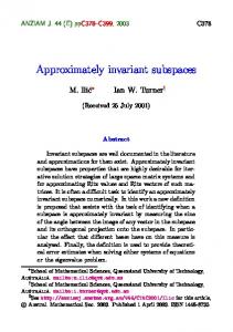
The proposed direct minimization algorithm 1 is realized in the recent density functional code bigDFT [45], which is implemented in the open source ABINIT package, a common project of the Universit´e Catholique de Louvain, Corning Incorporated, and other contributors [46, 23, 24, 15]. It relies on an efficient Fast Fourier Transform algorithm [19] for the conversion of wavefunctions between real and reciprocal space, together with a DIIS subspace acceleration. We demonstrate the convergence for the simple molecule cinchonidine (C19 H22 N2 O) of moderate size N = 55 for a given geometry of the nuclei displayed in figure 7.1. Despite the fact that the underlying assumptions in the present paper cannot be verified rigorously, the proposed convergence behavior is observed by all benchmark computations. The algorithm is experienced to be quite robust also if the HOMO-LUMO gap is relatively small.

28

Figure 7.1: Atomic geometry and electronic structure of cinchonidine

history size for DIIS = 6

steepest descent

1

2

10

10 hgrid = 0.3

0

10

hgrid = 0.3

hgrid = 0.45

−1

10

hgrid = 0.45

0

10

hgrid = 0.7

hgrid = 0.7

hgrid = 0.2

10

−2

absolute error

absolute error

−2

−3

10

10

−4

10

−4

10

−5

10

−6

10 −6

10

−8

10

−7

10

0

5

10

15

20

25 iter

30

35

40

45

0

50

5

10

15

20

25 iter

30

35

40

45

50

Figure 7.2: Convergence history for the direct minimization scheme (left) and with DIIS acceleration (right) for different mesh sizes. memory

runtime

6000

8000 DIIS hist = 6

DIIS, hist. size = 6

7000

steepest descent

5000

steepest descent 6000

4000

sec

MB

5000 3000

4000 2000

3000 1000

0 0.2

2000

0.25

0.3

0.35

0.4

0.45 hgrid

0.5

0.55

0.6

0.65

1000 0.3

0.7

0.35

0.4

0.45

0.5 hgrid

0.55

0.6

0.65

0.7

Figure 7.3: Memory requirements (left) and computing time (right) for direct minimization algorithm with and without DIIS acceleration.

29

For our computations, we have used a simple LDA (local density approximation) model proposed by [20] and norm-conserving non-local pseudopotentials [21]. The orbital functions ψi are approximated by Daubechies orthogonal wavelets with 8 vanishing moments based on an approximate Galerkin discretization [18]. For updating the nonlinear potential, the electron density is approximated by interpolating scaling functions (of order 16). The discretization error can be controlled by an underlying basic mesh size hgrid . In figure 7.2, we demonstrate the convergence of the present algorithm for 4 different choices of mesh sizes, where the error is given in the energy norm of the discrete functions. The initial guess for the orbitals is given by the atomic solutions. Except in case of nonsufficient resolution (hgrid = 0.7), where we obtain a completely wrong result, convergence is observed. If the discretisation is sufficiently good, we do not observe much difference in the convergence history for different mesh sizes. Since the convergence speed depends on the actual solution, it is only possible to observe that the convergence is bounded by a linear rate. The number of iterations is relatively moderate bearing in mind that one iteration step only requires matrix-vector multiplications with the Fock operator and not a corresponding solution of linear equations. The DIIS implemented in BigDFT accelerates the iteration by almost halving the number of iterations and the total computing time at the expense of additional storage capacities, see also figure 7.2. Further benchmark computations have already been performed and will be reported in different publications by the groups involved in the implementation of BigDFT.

References [1] P.-A. Absil, R. Mahony, R. Sepulchre, Optimization Algorithms on Matrix Manifolds, Princeton University Press,2007 [2] D. C. Allen, T. A. Arias, J. D. Joannopoulos, M. C. Payne, M. P. Teter, Iterative minimization techniques for ab initio total energy calculation: molecular dynamics and conjugate gradients, Rev. Modern Phys. 64 (4), 1045-1097,1992. [3] T. A. Arias, Multiresolution analysis of electronic structure: semicardinal and wavelet bases, Rev. Mod. Phys. 71, 267 - 311, 1999. [4] T. A. Arias, A. Edelman, S. T. Smith, The Geometry of Algorithms with Orthogonality Constraints, SIAM J. Matrix Anal. and Appl., Vol. 20, No. 2, pp. 303-353, 1999. [5] L. Armijo, Minimization of functions having Lipschitz continuous first partial derivatives, Pacific J. Math, 1966. 30

[6] M. Barrault, E. Cances, W. W. Hager, C. Le Bris, Multilevel domain decomposition for electronic structure calculations, Journ. Comp. Phys., Volume 222 , 1, 86-109, 2007. [7] T. L. Beck, Real-space mesh techniques in density-functional theory, Rev. Mod. Phys. 72, 1041 - 1080, 2000. [8] J. H. Bramble, J. E. Pasciak, A.V. Knyazev, A subspace preconditioning algorithm for eigenvector/eigenvalue computation, Advances in Computational Mathematics 6 (1996) 159-189, 1999. [9] E. Cances, M. Defranceschi, W. Kutzelnigg, C. Le Bris, Y. Maday, Computational Quantum Chemistry: A Primer, Handbook of Numerical Analysis, Volume X, Elsevier Science, 2003. [10] E. Cances, C. Le Bris, On the convergence of SCF algorithms for the Hartree-Fock equations, Mathematical Models and Methods in Applied Sciences, 1999. [11] W. Dahmen, T. Rohwedder, R. Schneider, A. Zeiser, Adaptive Eigenvalue Computation - Complexity Estimates, preprint, 2007 , obtainable at http://arxiv.org/abs/0711.1070 [12] M. Defranceschi, C. Le Bris, Mathematical Models and Methods for Ab Initio Quantum Chemistry, Lecture Notes in Chemistry, Springer, 2000. [13] R. M. Dreizler, E. K. U. Gross, Density functional theory, Springer, 1990. [14] C. Geiger, C. Kanzow, Theorie und Numerik restringierter Optimierungsaufgaben, Springer, 2002. [15] L. Genovese, A. Neelov, S. Goedecker, T. Deutsch, S. A. Ghasemi, A. Willand, D. Caliste, O. Zilberberg, M. Rayson, A. Bergman, R. Schneider, Daubechies wavelets as a basis set for density functional pseudopotential calculations, preprint, 2008, obtainable at http://arxiv.org/abs/0804.2583 [16] S. Goedecker, Wavelets and their Application for the Solution of Partial Differential Equation, Presses Polytechniques Universitaires et Romandes, Lausanne, 1998. [17] S. Goedecker, Linear Scaling Methods for the Solution of Schrodinger’s Equation, in: Handbook of Numerical Analysis Vol. X, Special volume on Computational Chemistry , P.G. Ciarlet and C. Le Bris (editors), North-Holland, 2003.

31

[18] A. Neelov, S. Goedecker, An efficient numerical quadrature for the calculation of the potential energy of wavefunctions expressed in the Daubechies wavelet basis, J. of. Comp. Phys. 217, 312-339, 2006. [19] S. Goedecker, Fast radix 2, 3, 4 and 5 kernels for Fast Fourier Transformations on computers with overlapping multiply-add instructions, SIAM J. on Scientific Computing 18, 1605, 1997. [20] S. Goedecker, C. J. Umrigar, Critical assessment of the self-interaction-corrected local-density-functional method and its algorithmic implementation, Phys. Rev. A 55, 1765 - 1771, 1997. [21] S. Goedecker, M. Teter, J. Hutter, Separable dual-space Gaussian pseudopotentials, Phys. Rev. B 54, 1703, 1996. [22] S. Goedecker, Linear scaling electronic structure methods , Rev. Mod. Phys. 71, 1085 - 1123, 1999. [23] X. Gonze, J.-M. Beuken, R. Caracas, F. Detraux, M. Fuchs, G.-M. Rignanese, L. Sindic, M. Verstraete, G. Zerah, F. Jollet, M. Torrent, A. Roy, M. Mikami, Ph. Ghosez, J.-Y. Raty, D.C. Allan, First-principles computation of material properties : the ABINIT software project, Computational Materials Science 25, 478-492, 2002. [24] X. Gonze, G.-M. Rignanese, M. Verstraete, J.-M. Beuken, Y. Pouillon, R. Caracas, F. Jollet, M. Torrent, G. Zerah, M. Mikami, Ph. Ghosez, M. Veithen, J.-Y. Raty, V. Olevano, F. Bruneval, L. Reining, R. Godby, G. Onida, D.R. Hamann, D.C. Allan, A brief introduction to the ABINIT software package Zeit. Kristallogr. 220, 558-562, 2005. [25] W. Hackbusch, Iterative solution of large sparse systems of equations, Springer, 1994. [26] T. Helgaker, P. Jorgensen, J. Olsen, Molecular electronic-structure theory, Wiley, New York, 2000. [27] P. Hohenberg, W. Kohn, Inhomogeneous Electron Gas, Phys. Rev. 136 p. 864-871, 1964. [28] A. V. Knyazev, K. Neymeyr, A geometric theory for preconditioned inverse iteration III: A short and sharp convergence estimate for generalized eigenvalue problems, Linear Algebra Appl. 358, 95–114. 2003. [29] E. H. Lieb, B. Simon, The Hartree-Fock Theory for Coulomb Systems, Commun. Math. Phys. 53, 185-194, 1977. 32

[30] P. L. Lions, Solution of the Hartree Fock equation for Coulomb Systems, Commum. Math. Phys. Volume 109, Number 1, 33-97, 1987. [31] D. Luenberger, Optimization by Vector Space Methods, Wiley, 1968. [32] C. Lubich, O. Koch, Dynamical Low Rank Approximation, preprint, Uni T¨ ubingen, 2008. [33] C. Moler, C. van Loan, Nineteen Dubious Ways to Compute the Exponential of a Matrix, Twenty-Five Years Later, SIAM Vol. 45, No.1, pp. 3-49, 2003. [34] K. Neymeyr, A geometric theory for preconditioned inverse iteration applied to a subspace, Math. Comp. 71, 197-216, 2002. [35] Y. Maday, G. Turinici, Error bars and quadratically convergent methods for the numerical simulation of the Hartree-Fock equations, Numerische Mathematik, Springer, 2003. [36] J. Nocedal, S. J. Wright, Numerical Optimization, Springer, 1999. [37] P. Pulay, Convergence Acceleration in Iterative Sequences: The Case of SCF Iteration, Chem. Phys. Lett. 73, 393, 1980. [38] D. Raczkowski, C. Y. Fong, P.A. Schultz, R. A. Lippert, E. B. Stechel, Unconstrained and constrained minimization, localization, and the Grassmann manifold: Theory and application to electronic structure Phys. Rev. B 64, 2001. [39] M. Reed and B. Simon, Methods of Modern Mathematical Physics IV: Analysis of Operators, Academic Press, 1978. [40] T. Rohwedder, R. Schneider, A. Zeiser, Perturbed preconditioned inverse iteration for operator eigenvalue problems with applications to adaptive wavelet discretization, preprint, 2007, obtainable at http://arxiv.org/abs/0708.0517. [41] Y. Saad, Analysis of some Krylov Subspace Approximations to the Matrix Exponential Operator, SIAM Journal on Numerical Analysis, Vol. 29, N0. 1., pp. 209-228, 1992. [42] Y. Shao, C. Saravanan, M. Head-Gordon, C. A. White, Curvy steps for density matrix-based energy minimization: Application to large-scale self-consistent-field calculations J. Chem. Phys. 118, 6144 ,2003. [43] A. Szabo, N. S. Ostlund, Modern Quantum Chemistry, Dover Publications Inc., 1992.

33

[44] R. B. Sidje, EXPOKIT: A Software Package for Computing Matrix Exponentials, ACM. Trans. Math. Softw., 24(1):130-156, 1998. [45] http://www-drfmc.cea.fr/sp2m/L Sim/BigDFT/index.en.html [46] http://www.abinit.org

Authors: Johannes Blauert Reinhold Schneider Thorsten Rohwedder Institute for Mathematics Technical University Berlin Straße des 17. Juni 135 10623 Berlin Germany

Alexej Neelov Institute of Physics University of Basel Klingelbergstrasse 82 4056 Basel Switzerland

34