Discovering Hierarchy in Reinforcement Learning with HEXQ Bernhard Hengst
[email protected] Computer Science and Engineering, University of New South Wales, UNSW Sydney 2052 AUSTRALIA
Abstract An open problem in reinforcement learning is discovering hierarchical structure. HEXQ, an algorithm which automatically attempts to decompose and solve a model-free factored MDP hierarchically is described. By searching for aliased Markov sub-space regions based on the state variables the algorithm uses temporal and state abstraction to construct a hierarchy of interlinked smaller MDPs.
higher level skills would be more efficient. In the rest of this paper we will describe the operation of a hierarchical reinforcement learning algorithm, HEXQ, which attempts to solve model-free MDPs more efficiently by finding and exploiting repeatable sub-structures in the environment. The algorithm is designed to automatically discover state and temporal abstractions, find appropriate sub-goals and construct a hierarchical representation to solve the overall MDP. As a running example we will use the taxi task (Dietterich, 2000a) to illustrate how the algorithm works. We also show results for a noisy Tower of Hanoi puzzle.
1. Introduction
2. Representation and Assumptions
Bellman (1961) stated that sheer enumeration would not solve problems of any significance. In reinforcement learning the size of the state space scales exponentially with the number of variables. Designers try to manually decompose more complex problems to make them tractable. Finding good decompositions is usually an art-form. Many researchers have either ignored where decompositions come from or pointed to the desirability of automating this task (Boutilier et al., 1999; Hauskrecht et al., 1998; Dean & Lin, 1995). More recently, Dietterich (2000b) concluded that the biggest open problem in reinforcement learning is to discover hierarchical structure.
We start with the usual formulation of a finite MDP with discrete time steps, states and actions (Sutton & Barto, 1998). The objective is to find an optimal policy by maximising the expected value of future discounted rewards represented by the action-value function, Q (Watkins & Dayan, 1992). We also employ semi-MDP theory (Puterman, 1994) which generalizes MDPs to models with variable time between decisions. We assume that the state is defined by a vector of d state variables, x = (x1 , x2 , ..., xd ). Large MDPs are naturally described in this factored form. In this paper we consider only negative reward non-discounted finite horizon MDPs (stochastic shortest path problems), but the algorithm has been extended to handle general finite MDPs. The issue of solving MDPs efficiently is largely orthogonal and complementary to the decomposition techniques discussed here. We have used simple one-step backup Q-learning throughout.
It was recognised by Ashby (1956) that learning is worthwhile only when the environment shows constraint. One type of constraint present in many environments is the repetition of sub-structures. Ashby stated that repetition is of considerable practical importance in the regulation of very large systems. Repetitions are commonplace. They are evident, for example, at the molecular level, in daily routines, in office layouts or even in just walking. One reason that reinforcement learning scales poorly is that sub-policies, such as walking, need to be relearnt in every context. It makes more sense to learn how to walk only once and then reuse this skill wherever it is required. A reinforcement learning agent that can find and learn reusable sub-tasks and in turn employ them to learn
HEXQ attempts to decompose a MDP by dividing the state space into nested sub-MDP regions. Decomposition is possible when (1) some of the variables in the state vector represent features in the environment that change at less frequent time intervals, (2) variables that change value more frequently retain their transition properties in the context of the more persistent variables and (3) the interface between regions can be controlled. For example, if a robot nav-
igates around four equally sized rooms with interconnecting doorways (Parr, 1998) the state space can be represented by the two variables, room-identifier and position-in-room. The room changes less frequently than the position. The position in each room needs to be represented consistently to allow generalisation across rooms, for example, by numbering cells from top to bottom, left to right in each room. Most representations naturally label repeated sub-structures in this way. Finally we need to be able to find sub-policies to exit through each doorway with certainty. This will become clearer in the next sections. In the absence of these conditions or when they are only partially present HEXQ will nevertheless solve the MDP discovering abstractions where it can. In the worst case it has to solve the ‘flat’ problem.
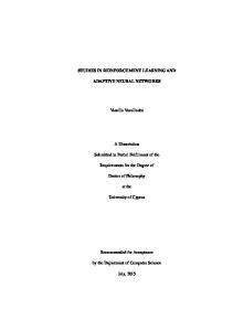
3. The Taxi Domain Dietterich (2000a) created the taxi task (Figure 1) to demonstrate MAXQ hierarchical reinforcement learning. For MAXQ the structure of the hierarchy is specified by the user. We will use the same domain to illustrate how hierarchical decomposition can be automated. We will keep our description of HEXQ general, but use the taxi domain to illustrate the basic concepts. We start by reviewing the taxi problem. In the taxi domain, a taxi, started at a random location, navigates around a 5-by-5 grid world to pick up and then put down a passenger. There are four possible source and destination locations, designated R, G, Y and B. We encode these 1, 2, 3, 4 respectively. They are called taxi ranks. The objective of the taxi agent is to go to the source rank, pick up the passenger, then navigate with the passenger in the taxi to the destination rank and put down the passenger. The source and destination ranks are also chosen at random for each new trial. At each step the taxi can perform one of six primitive actions, move one square to the north, south, east or west, pickup or putdown the passenger. A move into a wall or barrier leaves the taxi location unchanged. For a successful passenger delivery the reward is 20. If the taxi executes a pickup action at a location without the passenger or a putdown action at the wrong destination it receives a reward of -10. For all other steps the reward is -1. The trial terminates following a successful delivery. The taxi problem can be formulated as an episodic MDP with the 3 state variables: the location of the taxi (values 0-24), the passenger location including in the taxi (values 0-4, 0 means in the taxi) and the destination location (values 1-4). Deterministic actions will make the illustrations simpler. Results in section 7 are
Figure 1. The Taxi Domain.
based on stochastic actions. It is easy to see that for the taxi to navigate to one of the ranks the navigation policy can be the same whether it intends to pick up or put down the passenger. The usual ‘flat’ formulation of the MDP will solve the navigation sub-task as many times as it reoccurs in the different contexts. Dietterich has demonstrated how the problem can be solved more efficiently with sub-task reuse by designing a MAXQ hierarchy. We will now show how a hierarchy can be generated automatically to solve the problem.
4. Automatic Hierarchical Decomposition HEXQ uses the state variables to construct the hierarchy. The maximum number of levels in the hierarchy is the same as number of state variables. For the taxi domain there are three levels. The hierarchy is constructed, and levels are numbered from the bottom up. The bottom level, level 1, is associated with the variable that changes value most frequently. The rationale is that sub-tasks that are used most often appear at the lower levels and need to be learnt first. The first level is the only level that interacts with the environment using primitive actions. We start by observing one of the state variables. We choose this variable on the basis that it changes value most frequently. We now partition the states represented by the values of this variable into Markov regions. The boundaries between regions are identified by ‘unpredictable’ (see subsection 4.2) transitions which we call region exits. We then define sub-MDPs over these regions and learn separate policies to leave each region via its various exits. Whole regions are then abstracted and combined with the next most frequently changing state variable to form abstract states at the next level in the hierarchy. The exit policies just learnt become abstract actions
Table 1. Frequency of change for taxi domain variables over 2000 random steps.
Variable Passenger location Taxi location Destination
Frequency 4 846 0
Order 2 1 3
at this next level. At this stage we have a semi-MDP that has one less variable in the state description and only abstract actions. We now repeat the above process on the reduced problem forming at most one hierarchical level for each state variable. If this abstraction does not reduce the number of Q-values otherwise required we can simply take the cartesian product of the current level state with the next variable and continue the construction of the hierarchy with this combined state. The top level will have one sub-MDP which is solved by recursively calling other sub-MDP policies as its actions. Let us now describe this process in more detail. 4.1 Variable Ordering Heuristic Just as lines in the inner loop of programs are executed more frequently, variables that change value more frequently are associated with lower levels of the hierarchy. Conversely, variables that change less frequently set the context for the more frequently changing ones. The hierarchy is constructed from the bottom up starting with the variable that changes most frequently. To order the variables, we allow our agent to explore its environment at random for a set period of time and keep statistics on the frequency of change of each of the state variables. We then sort the variables based on their frequency of change. For the taxi, table 1 shows the frequency and order of each variable following a 2000 random action exploration run. 4.2 Discovering Repeatable Regions HEXQ starts by projecting the entire state space onto values of the variable that changes most frequently, limiting the state space to these values. Obviously, this makes the agent’s perception of the environment highly aliased. Nevertheless, HEXQ now proceeds to attempt to model the state transitions and rewards by exploring the environment, taking random actions. It models the state transitions as a directed graph (DG) in which the vertices are the state values and the edges are the transitions for each primitive action. Following a set period of exploration in this manner,
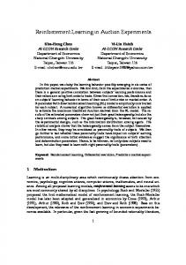
transitions that are unpredictable (called exits) are eliminated from the graph. Definition 1 An exit is a state-action pair (se , a) signifying that taking action a from state se causes an unpredictable transition. Transitions are unpredictable when (1) the state transition or reward function is not a stationary probability distribution, or (2) another variable may change value (or the task terminates). State se in definition 1 is a level e state (see subsection 4.3) and is referred to as an exit state. Action a is primitive for level 1 and abstract for all higher levels. An entry state is the state that is reached following an exit. For the taxi location variable, all states are entries because the taxi agent is restarted at any location at random following the episodic trial exit. We are left with a DG whose connections represent predictable transitions between values of the first level state variable. For the taxi example the directed graph for the taxi location variable is shown in Figure 2. The transitions labelled exits are not counted as edges. For example, taking action pickup or putdown in state 23 is not predictable because it may change the passenger location variable or reach the goal, respectively. However, we can predict the transitions anywhere else in the environment. State 7, for example, always transitions to state 2 on action north, 12 on south, 8 on east, 7 on west, 7 on pickup and 7 on putdown. We have only drawn one edge to represent multiple transitions between the same states in Figure 2 to avoid cluttering the diagram.
exits
exits 0
1
2
3
4
5
6
7
8
9
10
11
12
13
14
15
16
17
18
19
20
21
22
23
24
exits
exits
Figure 2. The directed graph of state transitions for the taxi location. Exits are non-predictable state transitions and not counted as edges of the graph.
We will now describe the general procedure to decompose a DG into regions that will meet our purpose for valid hierarchical state abstraction.
First we decompose the DG into strongly connected components (SCCs). An efficient linear time algorithm for this procedure can be found in Cormen et al. (1999). The SCCs, as abstracted nodes, form a directed acyclic graph (DAG). It is possible that there are many connected SCCs in the DAG. Because we only require that when we enter an abstract state we can leave via any exit, we can combine some SCCs to form regions. Whole regions will later be abstracted to form higher level states. Our objective is to maximise the size of these regions so as to minimise the number of abstract states. Following the coalition of SCCs into regions we may still have regions connected by edges from the underlying DAG. We break these by forming additional exits and entries associated with their respective regions and repeat the entire procedure until no additional regions are formed. The regions can be labelled arbitrarily. We use consecutive integers for convenience (see equation 1). A region, therefore, is a combination of SCCs such that any exit state in a region can be reached from any entry with probability 1. Regions are generally aliased in the environment. All the instances of these generic regions partition the total state space. Each region has a set of states, actions and predictable (i.e. Markov) transition and reward functions. We can therefore define a MDP over the region with an exit (or sub-goal) as a transition to an absorbing state. The solution to this ‘sub-MDP’ is a policy over the region that will move the agent out of an exit starting from any entry. We proceed to construct multiple sub-MDPs one for each unique hierarchical exit state (s1 , s2 , ...se ) in each region. Sub-MDP policies in HEXQ are learnt on-line, but a form of hierarchical dynamic programming could be used directly as the sub-task models have already been uncovered. In the taxi example, the above procedure finds one hierarchical level 1 region as reflected in figure 2. This region has 8 exits. They are: (s1 (s1 (s1 (s1
= 0, a = pickup), = 4, a = pickup), = 20, a = pickup), = 23, a = pickup),
(s1 (s1 (s1 (s1
= 0, a = putdown), = 4, a = putdown), = 20, a = putdown), = 23, a = putdown).
As there are 4 hierarchical exit states we create 4 subMDPs at level 1 and solve them. 4.3 State and Action Abstraction We are now in the position to tackle the second level in the hierarchy. The process is similar to the first level in that we will be searching for repeatable regions. Except now the states and actions are based on
abstractions from the first level. We define abstract states at the second level as the cartesian product of the region labels and values of the next state variable in the frequency ordering. A convenient numerical method for generating abstract state values is as follows: where se+1
se+1 = |re |xj + re
(1)
=
abstract state value at level e+1
e
|r | xj
= =
number of regions at level e next most frequent state variable value
re
=
region label from level e
The abstract actions available in each of these abstract states are the policies leading to region exits at the level below. Abstract actions are similar to composite actions in Dietterich (2000a). The effect of taking an abstract action in state se is to invoke and execute the associated level e − 1 sub-MDP policy.
For the taxi example there is only one region at level 1 which we label 0. When we apply equation (1), the level 2 hierarchy states, s2 , simply correspond to the values of the passenger location. We therefore generate 5 states at level 2. There are 8 abstract actions which are the policies that lead to the exits listed previously. It is generally the case that different abstract states have different abstract actions. Also, because abstract actions can take varying primitive time periods to execute, we now have a semi-Markov decision problem. This semi-MDP has one less variable than the original MDP and uses only abstract actions.
2
1
3
(s1=4, a=pickup)
(s1=20, a=pickup)
4
(s1=23, a=pickup)
(s1=0, a=pickup) 0
Level 2 exits
{
(s2 = 0, (s1 = 0, a = putdown)) (s2 = 0, (s1 = 4, a = putdown)) (s2 = 0, (s1 = 20, a = putdown)) (s2 = 0, (s1 = 23, a= putdown))
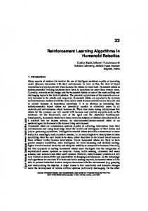
Figure 3. State transitions for the passenger location variable at level 2 in the hierarchy. There are 4 exits at level 2.
We repeat the level 1 procedure, finding regions and exits using the abstract states and actions at level 2.
For the taxi, the region and exits at level 2 are shown in figure 3. Note that the actions are abstract and labelled using the exit notation from the first level. There are 4 exits at level 2. They are also shown in figure 3. For example, exit (s2 = 0, (s1 = 23, a = putdown)) means: with the passenger in the taxi, navigate to location s1 = 23 and putdown the passenger. This is an exit because it may or may not lead to the goal, depending on the destination location. We generate 4 sub-MDPs for level 2 given the 4 unique hierarchial exit states.
ecuted using primitive actions to move the taxi from location s1 = 5 to the pickup location s1 = 23 and the pickup action is executed on exit. Level 1 returns control to level 2 where the state has transitioned to s2 = 0. Level 2 now completes its instruction and takes abstract action (s1 = 20, a = putdown). This again invokes level 1 primitive actions to move the taxi from location s1 = 23 to s1 = 20 and then putdown to exit. Control is returned back up the hierarchy and the trial ends with the passenger delivered correctly.
In this way we generate one level of hierarchy for each variable in the original MDP. The only change to the predictability criteria is that we only test state variables for change from the ones we have not yet processed. When we reach the last state variable we solve the top level sub-MDP represented by the final abstract states and actions which solves the overall MDP.
5. Hierarchical Value Function
1
2
3
4
(s2 = 0, (s1 = 0, a = putdown))
(s2 = 0, (s1 = 4, a = putdown))
(s2 = 0, (s1 = 20, a = putdown))
(s2 = 0, (s1 = 23, a = putdown))
HEXQ is similar to MAXQ in its approach to hierarchical execution using a decomposed value function, but there are important differences. The motivation for these new decomposition equations is that they automatically solve the hierarchical credit assignment problem (Dietterich, 2000a) by relegating non-repeatable sub-task rewards further up the hierarchy where they can be ‘explained’. The equations also reduce nicely to the usual Q and value functions for ‘flat’ MDPs if there is only one variable in the state vector. Definition 2 The recursively optimal hierarchical exit Q-function Q∗em (se , a) at level e in sub-MDP m is the expected value after completing the execution of (abstract) action a starting in (abstract) state se and following the optimal hierarchical policy thereafter. ! ∗ Q∗em (se , a) = Tsae s! [Rsae + Vem (s" )] (2) s!
where
Figure 4. The top level sub-MDP for the taxi domain showing the abstract actions leading to the goal.
Tsae s! Rsae
The top level sub-MDP for variable destination is shown in figure 4. Note the nesting in the description of abstract actions.
s"
To illustrate the execution of a competent taxi agent on the hierarchically decomposed problem, let us assume the taxi is initially located randomly at cell 5, the passenger is on rank 4 and wants to go to rank 3. In the top level sub-MDP, the taxi agent perceives the passenger destination as 3 and takes abstract action (s2 = 0, (s1 = 20, a = putdown)). This sets the subgoal state at level 2 to s2 = 0 or in English, pick up the passenger first. At level 2, the taxi agent perceives the passenger location as 4, and therefore executes abstract action (s1 = 23, a = pickup). This abstract action sets the sub-goal state at level 1 to taxi location s1 = 23, i.e. rank 4. The level 1 policy is now ex-
= P r{s" |se , a} = E{primitive reward after a|se , a} !
!
= hierarchical next state = (s1 , ..., se )
Note that Q includes the expected primitive reward immediately after sub-task exit, but does not include any rewards accumulated while executing the subtasks. The name HEXQ is derived from this function. The recursively optimal hierarchical value function decomposition is given by: " # ∗ ∗ ∗ e Vem (s) = max Ve−1,m (3) e−1 (a) (s) + Qem (s , a) a
where me−1 (a)
=
subMDP implementing action a
The manner in which regions are formed has ensured that no action will exit a sub-MDP unintentionally.
For our special case of stochastic shortest path problems we avoid the introduction of the pseudo-reward functions (Dietterich, 2000a). We can therefore update all region sub-policies concurrently using off-policy backups, similarly to all goals updating (Kaelbling, 1993).
6. Stochastic Considerations
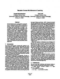
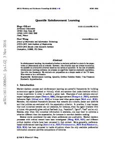
7. Results Figure 5 compares the performance of HEXQ against MAXQ and a ‘flat’ learner on a stochastic taxi task, with each of the four navigation actions performing as intended 80% of the time and 20% of the time moving the taxi randomly to the left or right of the intended action.
HEXQ handles stochastic actions and rewards. The aspects that need attention are explained in the following two sections.
Exits can also occur (see definition 1) when a state transition or reward is not predictable and a higher level state variable does not change value. In the deterministic case it is easy to determine these exits. We only need to find a transition to two different next states or reward values for the same action to trigger an exit condition. In the stochastic case we need to record statistics and test the hypothesis that the reward and state transitions (R and T functions in equation 2) come from different probability distributions in some contexts. In theory it is possible to determine this to any degree of accuracy given that we can test all the individual contexts represented by the higher level variables. In practice this is intractable, because the combinations of higher level variables can grow exponentially. Instead, we keep the transition statistics over a shorter period of time and compare these to their long term average. The objective is to explicitly test whether the probability distribution is stationary. We use a binomial distribution based on average probabilities to test when a temporally close sample of each transition is outside an upper confidence limit. When this happens we declare an exit. Similarly, to detect reward function non-stationarity we use the Kolmogorov-Smirnov test. 6.2 Hierarchical Greedy Policy A sub-MDP will stubbornly attempt to exit a region by the exit determined from the level above even though the agent may have slipped closer to another exit that is now more optimal (Hauskrecht et al., 1998). The solution is to re-evaluate the optimum policy at every level after every step. This is only possible after the uninterrupted exit policies have been learnt and is referred to as a hierarchical greedy policy by Dietterich (2000a).
Steps to Passenger Delivery
6.1 Detecting Non-Markov Transitions
1000
Flat 100
HEXQ MAXQ 10 100
200
300
400
500
Trials
Figure 5. Performance of HEXQ vs a ‘Flat’ learner and MAXQ for the stochastic taxi.
The graph shows the number of primitive time steps required to complete each successive trial averaged over 100 runs. For all experiments the Q-learning rate was set at 0.25. The initial Q-values were set to 0 and all actions were greedy, except for those during hierarchy construction as described previously. Exploration is implicitly forced by the initial Q-values and the stochastic actions. HEXQ performance improves in distinct stages as each level of the hierarchy is constructed. After about 41 trials it surpasses the performance of the ‘flat’ learner. While the ‘flat’ learner can start to improving performance during the first trial, HEXQ must first order the variables and find exits at the first level before it can improve its performance. HEXQ then learns more rapidly as it transfers sub-task skills. The investment in hierarchy construction ‘breaks even’ at 220 trials, where the cumulative number of time steps for both the ‘flat’ learner and HEXQ are equal. With its additional background knowledge MAXQ learns very rapidly. In our version of MAXQ the slower convergence evident is caused by learning the Q-values at all levels simultaneously. Higher level Q-values are initially learnt with inflated costs from the lower level partially learnt policies. In terms of storage requirements for the value function, a ‘flat’ learner uses a table of 500 states and 6 actions
= 3000 values. HEXQ requires 4 MDPs at level 1 with 25 states and 6 actions = 600 values. 4 MDPs at level 2 with 5 states and 8 actions = 160 values. 1 MDP at level 3 with 4 states and 4 actions = 16 values. A total of 776 values. MAXQ by comparison requires only 632 values. HEXQ, of course, is not told which actions to apply at different levels and must discover these for itself. As a second example the performance of HEXQ is compared to a ‘flat’ learner for a noisy 3 pin Tower of Hanoi puzzle (ToH) with 7 disks. The state variables are the disks. Their values represent the pin positions. Each disk can be moved to another pin but only if no other disk is moved in the process and the disks on each pin remain ordered in size with the smallest on top. Actions are defined by disk and target pin. An example action is move-disk3-to-pin2. There are three such actions per disk, at total of 21. The actions are stochastic in the sense that having picked up a disk there is an 80% probability that an intended legal move will succeed and a 20% probability that the disk will attempt to slip randomly to another pin. For illegal moves the disks remains in situ. The reward is -1 per move. The goal is to move all the disks to pin 3. Disks are randomly (but legally) placed on the pins at the start of each trial. The learners are model-free.
1000000
Mov es to reach goal
100000
Flat 10000
1000
HEXQ
100 0
1000
2000
3000
4000
Trials
Figure 6. Performance of HEXQ vs a ‘Flat’ learner for a stochastic Tower of Hanoi puzzle with 7 disks averaged over 10 runs and smoothed.
From figure 6 we see that HEXQ learns the 7 disk ToH in a fraction of number of trials of the ‘flat’ learner. HEXQ takes about half the number of steps to converge compared to the ‘flat’ learner. The recursive value function implements a depth first search which becomes expensive with 7 levels. This issue is shared with MAXQ. A reasonable approach is to only evaluate the function to a certain depth. By analogy, in
planning a trip from New York to Sydney we do not take into consideration which side of the bed to get out of on our way to the bathroom on the day of departure. In this example we have limited the search to a depth of only 1. This is possible in the ToH because the recursive constraints are such that the values below level 1 cannot change the outcome. The ToH has alternative action representations. Move-fromPin-toPin would require only 6 actions. With this representation HEXQ can quickly learn the deterministic n disk ToH in time complexity of O(n2 ) and space complexity of O(n). With general stochastic actions this representation fails to decompose because every action for every disk state is an exit.
8. Limitations and Future Work While HEXQ will not perform any worse than a ‘flat’ learner, it relies on certain constraints in the problem to allow it to find decompositions. If a subset of the variables can form sub-MDPs and we can find policies to reach their exits with probability 1 then HEXQ can find a decomposition. To find sub-MDPs it is necessary that some variables change on a longer timescale. The requirement to be able to exit with certainty ensures that learnt sub-tasks do not present any uncontrollable surprises to higher level tasks. This means that some benign problems, such as navigating around a multi-room domain with stochastic actions that slip in all directions, will not HEXQ decompose. We leave to future work automatically finding conditions under which the exit-with-certainty constraint can be relaxed. Problem characteristics may result in the discovery of a large number of exits. For example, if a doorway is modelled with three exit states, indicating that it is possible to exit either left, right or centre, HEXQ will generate and solve 3 sub-MDPs. A designer can choose to combine exits and only generate one subMDP. An improvement would be to extend HEXQ to automatically combine exits leading to the same next state. Exit combination heuristics based on general transition properties, such as entering the same next region or having small Q-value differences suggest themselves. Exit combining will make some problems decomposable as a composite exit may now be reached with probability one. We leave to further study the tradeoff between intra-region value improvement and inter-region value deterioration as exits are combined. The two heuristics employed by HEXQ are (1) variable ordering and (2) finding non-stationary transitions. If the frequency order of variables is changed HEXQ may still be able to partially decompose the MDP, but in
most cases less efficiently. Decompositions under different variable combinations and orderings is further discussed in Hengst (2000). An independent slowly changing random variable would be sorted to the top level in the hierarchy by this heuristic and the MDP will fail to decompose as it is necessary to explore the variable’s potential impact. Further research may be better directed towards selecting relevant variables for the task at hand rather than finding better sorting heuristics. For the second heuristic the penalty for recognising extra exits is simply to generate some additional overhead for HEXQ. These exits will require new policies to be learnt and they in turn will need to be explored as new abstract actions in the next level up the hierarchy. This does not detract from the quality of the solution in terms of optimality. If exits are missed the solution may not be effected at all. Alternatively, it may be more circuitous or, in the worst case, fail altogether. It would be possible to incorporate recovery procedures in HEXQ when new exits are belatedly discovered. At this stage we rely on HEXQ to find all relevant exits. For deterministic shortest path problems HEXQ will find a globally optimal policy. With stochastic actions HEXQ, as MAXQ is recursively optimal.
9. Conclusion HEXQ has tackled the problem of discovering hierarchical structure in stochastic shortest path factored MDPs. HEXQ will decompose MDPs if it can find nested sub-MDPs where there are policies to reach any exit with certainty. Generally it will perform well on problems where it can identify large regions, few exits and many contexts in which the sub-tasks are required. HEXQ has automated work that is usually required to be performed by a designer. This includes defining sub-tasks, finding sets of actions that can be performed in each sub-task, finding sub-task termination conditions or sub-goals, finding usable state and temporal abstractions and assigning credit hierarchically. Work is ongoing to generalise HEXQ, building on the key idea of discovering Markov sub-spaces, to handle hidden state and selective perception. We believe the discovery and manipulation of hierarchical representations will prove essential for lifelong learning in autonomous agents.
References Ashby, R. (1956). Introduction to cybernetics. London: Chapman & Hall.
Bellman, R. (1961). Adaptive control processes: A guided tour. Princeton, NJ: Princeton University Press. Boutilier, C., Dean, T., & Hanks, S. (1999). Decisiontheoretic planning: Structural assumptions and computational leverage. Journal of Artificial Intelligence Research, 11, 1–94. Cormen, T. H., Leiserson, C. E., & Rivest, R. L. (1999). Introduction to algorithms. Cambridge Massachusetts: MIT Press. Dean, T., & Lin, S. H. (1995). Decomposition techniques for planning in stochastic domains (Technical Report CS-95-10). Department of Computer Science Brown University. Dietterich, T. G. (2000a). Hierarchical reinforcement learning with the MAXQ value function decomposition. Journal of Artificial Intelligence Research, 13, 227–303. Dietterich, T. G. (2000b). An overview of MAXQ hierarchical reinforcement learning. SARA (pp. 26–44). Hauskrecht, M., Meuleau, N., Kaelbling, L. P., Dean, T., & Boutilier, C. (1998). Hierarchical solution of Markov decision processes using macro-actions. Fourteenth Annual Conference on Uncertainty in Artificial Intelligence (pp. 220–229). Hengst, B. (2000). Generating hierarchical structure in reinforcement learning from state variables. PRICAI 2000 Topics in Artificial Intelligence (pp. 533–543). San Francisco: Springer. Kaelbling, L. P. (1993). Hierarchical learning in stochastic domains: Preliminary results. Machine Learning Proceedings of the Tenth International Conference (pp. 167–173). San Mateo, CA: Morgan Kaufmann. Parr, R. E. (1998). Hierarchical control and learning for Markov decision processes. Doctoral dissertation, University of California at Berkeley. Puterman, M. L. (1994). Markov decision processes: Discrete stochastic dynamic programming. New York, NY: John Whiley & Sons, Inc. Sutton, R. S., & Barto, A. G. (1998). Reinforcement learning: An introduction. Cambridge, Massachusetts: MIT Press. Watkins, C. J. C. H., & Dayan, P. (1992). Technical note: Q-learning. Machine Learning, 8, 279–292.