Discovering Word Senses from Text Using Random Indexing Niladri Chatterjee1 and Shiwali Mohan2 1
Department of Mathematics, Indian Institute of Technology Delhi, New Delhi, India 110016
[email protected] 2 Yahoo! Research and Development India, Bangalore, India 560 071
[email protected]
Abstract. Random Indexing is a novel technique for dimensionality reduction while creating Word Space model from a given text. This paper explores the possible application of Random Indexing in discovering word senses from the text. The words appearing in the text are plotted onto a multi-dimensional Word Space using Random Indexing. The geometric distance between words is used as an indicative of their semantic similarity. Soft Clustering by Committee algorithm (CBC) has been used to constellate similar words. The present work shows that the Word Space model can be used effectively to determine the similarity index required for clustering. The approach does not require parsers, lexicons or any other resources which are traditionally used in sense disambiguation of words. The proposed approach has been applied to TASA corpus and encouraging results have been obtained.
1 Introduction Automatic disambiguation of word senses has been an interesting challenge since the very beginning of computational linguistics in 1950s [1]. Various clustering techniques, such as bisecting K-means [2], Buckshot [3], UNICON [4], Chameleon [5], are being used to discover different senses of words. These techniques constellate words that have been used in similar contexts in the text. For example, when the word ‘plant’ is used in the living sense, it is clustered with words like ‘tree’, ‘shrub’, ‘grass’ etc. But when it is used in the non-living sense, it is clustered with ‘factory’, ‘refinery’ etc. Similarity between words is generally defined with the help of existing lexicons, such as WordNet [6], or parsers (e.g. Minipar [7] ). Word Space model [8] has long been in use for semantic indexing of text. The key idea of Word Space model is to assign vectors to the words in high dimensional vector spaces, whose relative directions are assumed to indicate semantic similarity. The Word Space model has several disadvantages: sparseness of the data and high dimensionality of the semantic space when dealing with real world applications and large size data sets. Random Indexing [9] is an approach developed to deal with the problem of high dimensionality in Word Space model. In this paper we attempt to show that the Word Space model constructed using Random Indexing can be used efficiently to cluster words, which in turn can be used A. Gelbukh (Ed.): CICLing 2008, LNCS 4919, pp. 299–310, 2008. © Springer-Verlag Berlin Heidelberg 2008
300
N. Chatterjee and S. Mohan
for disambiguating the sense of the word. In a Word Space model the geometric distance between the words is indicative of the semantic similarity of the words. We use soft Clustering by Committee (CBC) [7] algorithm to congregate similar words. It can discover the less frequent senses of a word, and thereby avoids discovering duplicate senses. The typical CBC algorithm uses resources, such as MiniPar, to determine similarity between words. However, the advantage of Random Indexing is that it uses minimal resources. Here similarity between the words is determined based on their usage in the text, and this eliminates the need of using any lexicon or parser. Further, Random Indexing helps in dimensionality reduction as it involves simple computations e.g. vector addition and thus is less expensive than other techniques such as Latent Semantic Indexing [10].
2 The Word Space Model and Random Indexing The meaning of a word is interpreted by the context it is used in. Word Space model [8] is a spatial representation of word meaning. In the following subsections we describe these models. 2.1 Word Space Model In this model the complete vocabulary of any text (containing n words) can be represented in an n-dimensional space in which each word occupies a specific point in the space, and has a vector associated with it defining its meaning. The words are placed on the Word Space model according to their distributional properties in the text, such that: 1. 2.
The words that are used within similar group of words (i.e. in similar context) should be placed nearer to each other. The words that lie closer to each other in the word space have similar meanings, while the words distant in the word space are dissimilar in their meanings.
2.1.1 Vectors and Co-occurrence Matrix – Geometric Representation of Distributional Information A context of a word is understood as the linguistic surrounding of the word. As an illustration, consider the following sentence: A friend in need is a friend indeed. Table 1. Co-occurence matrix for the sentence A friend in need is a friend indeed
Word a friend in need is indeed
a 0 2 0 0 1 0
friend 2 0 1 0 0 1
Co-occurrents in need is indeed 0 0 1 0 1 0 0 1 0 1 0 0 1 0 1 0 0 1 0 0 0 0 0 0
Discovering Word Senses from Text Using Random Indexing
301
If we define the context of a word as one preceding and one succeeding word, then the context of ‘need’ is ‘in’ and ‘is’, and the context of ‘a’ is ‘is’ and ‘friend’. To tabulate this context information a co-occurrence matrix of the following form is created, in which the (i, j)th element denotes the number of times word i occurs in the context of word j within the text. Here, the context vector for ‘a’ is [0 2 0 0 1 0] and for ‘need’ is [0 0 1 0 1 0], determined by the corresponding rows of the matrix. A context vector thus obtained can be used to represent the distributional information of the word into the geometrical space. This is similar to each word being assigned a unique unary vector of dimension six (here), called index vector. The context vector for a word can be obtained by summing up the index vectors of the words on the either side of it. An index vector [ 0 0 0 0 1 0 ] can be assigned to the word ‘is’ ; and the word ‘in’ can be assigned an index vector [0 0 1 0 0 0]. These two in turn can be summed up to get the context vector for ‘need’ [0 0 1 0 1 0]. 2.1.2 Similarity in Mathematical Terms Context vectors give the location of the word in the word space. In order to determine how similar the words are in their meaning, a similarity measure has to be defined. Various schemes, e.g. scalar product of vectors, Euclidean distance, Minkowski metrics [9], are used to compute similarity between vectors corresponding to the words. We have used cosine of the angles between the two vectors x and y to compute normalized vector similarity. The cosine angle between vectors x and y is defined as: sim cos
x. y ( x, y ) = = | x || y |
∑ ∑
n i =1
x
2 i
n i =1
xi yi
∑
n i =1
y i2
(1)
The cosine measure is the most frequently utilized similarity metric in word-space research. The advantage of using cosine metric over other metrics is that it provides a fixed measure of similarity, which ranges from 1 (for identical vectors), to 0 (for orthogonal vectors) and -1 (for vectors pointing in the opposite directions). Moreover, it is also comparatively efficient to compute. 2.1.3 Problems Associated with Implementing Word Spaces The dimension n used to define the word space corresponding to a text document is equal to the number of unique words in the document. Therefore, the number of dimensions increases as the size of text increases. Thus computational overhead increases rapidly with the size of the text. The other problem is of data sparseness. The majority of cells in the co-occurrence matrix constructed corresponding to a document will be zero. The reason is that most of the words in any language appear in limited contexts only, i.e. the words they co-occur with are very limited. While dimensionality reduction does make the resulting lower-dimensional context vectors easier to compute, it does not solve the problem of initially having to collect a potentially huge co-occurrence matrix. Even implementations, such as Latent Semantic Analysis [11], that use powerful dimensionality reduction, need to initially collect the words-by-documents or words-by-words co-occurrence matrix. Random
302
N. Chatterjee and S. Mohan
Indexing (RI) described below removes the need for the huge co-occurrence matrix. Instead of first collecting co-occurrences in a matrix and then extracting context vectors from it, RI incrementally accumulates context vectors, which can then be assembled into a co-occurrence matrix. 2.2 Random Indexing Random Indexing [9] is based on Pentti Kanerva’s [11] work on sparse distributed memory. Random Indexing accumulates context vectors in a two step process: 1. Each word in the text is assigned a unique and randomly generated vector called the index vector. The index vectors are sparse, high dimensional and ternary (i.e. 1, -1, 0). Each word is also assigned an initially empty context vector which has the same dimensionality (r) as the index vector. 2. The context vectors are then accumulated by advancing through the text one word taken at a time, and then adding the context's index vector to the focus word's context vector. When the entire data is processed, the r-dimensional context vectors are effectively the sum of the words' contexts. For illustration we again take the example of the sentence ‘A friend in need is a friend indeed’. Let the dimension r of the index vector be 10, and the context be defined as one preceding and one succeeding word. Let ‘friend’ be assigned a random index vector: [0 0 0 1 0 0 0 0 -1 0 ], and ‘need’ be assigned a random index vector: [0 1 0 0 -1 0 0 0 0 0]. Then to compute the context vector of ‘in’ we need to sum up the index vectors of its context. Since the context is defined as one preceding and one succeeding word, the context vector of ‘in’ is the sum of index vectors of ‘friend’ and ‘need’ , and is equal to [0 1 0 1 -1 0 0 0 -1 0]. If a co-occurrence matrix has to be constructed, r-dimensional context vectors can be collected into a matrix of order [w, r], where w is the number of unique words, and r is the chosen dimensionality of each word. Note that this is similar to constructing an n-dimensional unary context vector that has a single 1 in different positions for different words, and n is the number of distinct words. These n dimensional unary vectors are orthogonal, whereas the r-dimensional random index vectors are nearly orthogonal [13]. Choosing RI is an advantageous tradeoff between the number of dimensions and orthogonality, as the r-dimensional random index vectors can be seen as approximations of the n-dimensional unary vectors. The context vectors computed on the language data are used in mapping the words onto the word space. Compared to other Word Space methodologies, Random Indexing approach gives us the following advantages: First, it is an incremental method, i.e. the context vectors can be used for similarity computations even when only a small number of examples have been encountered. By contrast, most other word space methods require the entire data to be sampled before similarity computations can be performed. Second, it uses fixed dimensionality, which means that new data does not increase the dimensionality of the vectors. Increasing dimensionality can lead to significant scalability problems in other word space methods.
Discovering Word Senses from Text Using Random Indexing
303
Third, it uses implicit dimension reduction, since the fixed dimensionality is much lower than the number of words in the data. This leads to a significant gain in processing time and reduction in memory consumption. Typically, the dimension r is about 10% of n, the number of unknown words.
3 Clustering by Committee Clustering by Committee [7] has been specially designed for Natural Language Processing purposes. The hard version of CBC, in which a word is assigned to exactly one cluster, is typically used for document retrieval. We use a soft version of the above in word sense disambiguation. The advantage thereby is that, it allows fuzzy clustering, and consequently, the words are assigned to more than one cluster, perhaps with varying degree of membership. It consists of three phases: Phase I - Generation of a similarity matrix Here, a similarity index [7] between words is defined, and a similarity matrix is generated from the words appearing in the text, in which each cell contains the numerical value of the similarity between any pair of words. Phase II - Formation of committees The second phase of the clustering algorithm takes in as input the list of words to be clustered and the similarity matrix. It recursively finds tight clusters called committees, scattered in the similarity space. Each committee can be thought of as the representation of a context or a sense. Each committee is assigned a centroid vector which is the average of the vectors of the words contained by them. The algorithm tries to form as many committees as possible on the condition that each newly formed committee is not very similar to any existing committee (i.e. the similarity is not more than a given threshold θ1). If the condition is violated, the committee is discarded. The similarity between two committees is computed by determining the cosine metric between the centroid vectors of the respective committees. Next, it identifies the residue words that are not covered by any committee. A committee is said to cover a word if the word’s similarity to the centroid of the committee exceeds some high similarity threshold (i.e. greater than another given threshold θ2). The algorithm then attempts to find recursively more committees among the residue words. The output of the algorithm is the union of all committees found in each recursive step. Committees are the cores of the clusters to which words are successively added in Phase III as explained below. The committees do not change after their formation. Phase III – Assigning of word to its most similar committee In the final phase of the algorithm each word is assigned to its most similar clusters. The word is assigned to a cluster if its similarity to the committee that forms the core of the cluster exceeds a given threshold σ. The cluster now represents the context the word has been used in. Once a word has been assigned to a cluster, the centroid of the committee is subtracted from the context vector of the word. This enables the
304
N. Chatterjee and S. Mohan
algorithm to find the less frequent context of the word. This phase is similar to Kmeans clustering. Like K-means the words are assigned to clusters whose centroids are closest to the word. However, unlike K-means clustering, the word is not added to the committee itself, but to the cluster surrounding it, so the centroids remain constant. This differentiates it from K-means clustering algorithm. Once an element is assigned to its most similar cluster, the centroid of the committee is subtracted from the context vector of the concerned word. The context vector of the word, as discussed in Section 3.2, is the sum of all the contexts the word may have appeared in, in the text. If one of the contexts is removed from the context vector of the word, the similarity of the word with other committees increases thus allowing the algorithm to discover other less frequent senses of the word.
4 Experimental Setup We conducted our experiments on the TASA corpus [8]. The corpus is 56 Mb in size and contains 10,802,187 unique words after stemming. It consists of high school level English text and is divided into paragraphs on various subjects, such as science, social studies, language and arts, health and business. The paragraphs are of 150-200 words each. To use them in our experiments we did the following preprocessing: The words appearing in the text were stemmed using Porter’s stemming algorithm [13] to reduce the word to their base forms. This reduced the number of word forms considerably. Stop words [14] such as is, are, has, have etc. were removed from the text as these words do not contribute to the context. 4.1 Mapping of Words onto Word Space Model Each word in the document was initially assigned a unique randomly generated index vector of the dimension r = 1500, with ternary values (1, -1, 0). The index vectors were so constructed that each vector of 1500 units contained eight randomly placed 1s and eight randomly placed -1s, rest of the units were assigned 0. Each word was also assigned an initially empty context vector of dimension 1500. We conducted experiments with different context window sizes. The results are presented in Section 5. The context of a given word was restricted in one sentence, i.e. windows across sentences were not considered. In case where the window is extended in the preceding or the succeeding sentence, a unidirectional window was used. Once the context vectors for the words were obtained, similarity between words was determined by computing the cosine metric between the corresponding context vectors. 4.2 Implementation of Clustering Algorithm Once we acquired the semantic similarities of the words in the text, we ran soft Clustering by Committee algorithm to find the committees present in the text and to assign words to their most similar committees. Fig. 1 gives a description of the algorithm. The experiments were conducted for varying values of parameters θ1, θ2, σ (defined in Section 3), and results are presented in Section 5.
Discovering Word Senses from Text Using Random Indexing
Phase 1 let E be S be the assign E(i) and
305
the list of unique words (n) in the text similarity matrix (n X n) values to S(i,j), by computing the cosine metric between E(j)
Phase 2 let S be the similarity matrix generated from phase 1 let E be the list of words to be clustered let C be the list of committees discover_committees (S, E,θ1,θ2) { for each element e Є E { cluster elements for S using average link clustering} for each discovered cluster c{ compute avgsim(c) //average pairwise similarity between elements in c compute score: |c| × avgsim(c) //|c| is the number of elements in c} store the highest-scoring cluster in a list L. sort the clusters in L in descending order of their scores. let C be a list of committees. for each cluster c Є L{ compute the centroid of c if c’s similarity to the centroid of each committee previously added to C is below a threshold θ1, add c to C.} If L is empty, return C. else{ For each element e Є E{ If e’s similarity to every committee in C is below threshold θ2, add e to a list of residues R } If R is empty, return C else discover_committees (S, R, θ1,θ2)} } Phase 3 let X be a list of clusters initially empty let C be the list of committees from phase 3 while S is not empty { let c Є S be the most similar committee to e if the similarity(e, c) < σ, exit the loop if c is not similar to any cluster in C { assign e to c remove from e the centroid vector of c;} remove c from S}
Fig. 1. Soft Clustering by Committee algorithm
5 Results and Discussion As mentioned in Section 4, the experiments presented in this paper were conducted using the untagged TASA corpus. We selected around 50 paragraphs each from the categories: Science, Social Science and Language and Arts. The paragraphs were selected randomly from the corpus. They contained 1349 unique words of which 104 were polysemous words. The results of the different stages of the algorithm are summarized below.
306
N. Chatterjee and S. Mohan
Phase 1 This phase determined the similarity index between words. Words such as chlorine and sodium were found to have similarities as high as 0.802 with a context window of size two. We realized that the training data for most of the sample words was small. Only two paragraphs of about 150 words each contained the words chlorine and sodium, still the similarity index was high. Phase II Here, the committees present in the text are identified. In total 834 committees in all were discovered. Table 2 shows some the committees with formed with the highest scores. Table 2. The committees with highest scores Type of Text Science
Social Science Language and Arts
Cluster Type Common elements Sources of light Places to live Water resources Body movements Colours
Cluster formed {chlorine, sodium, calcium, iron, wood, steel} {sun, bulb, lamp, candle, star} {country, continent, island, state, city} {nile, river, pacific, lake, spring} {dance, walk, run, slide, clap} {red, yellow, blue, green, black}
Phase III This phase assigned the words to different clusters. Table 3 shows some of the words and their discovered senses/committees. Note that some of the words belong to more than one cluster, suggesting that they are used in more than one sense. Table 3. Some of the words and their discovered senses/committees Polysemous Word Capital Water
Plank
Clusters Sense 1- money, donation, funding Sense 2- camp, township, slum Sense 1- liquid, blood, moisture Sense 2- ocean, pond, lagoon Sense 3-tide, surf, wave, swell Sense 1- bookcase, dining table, paneling Sense 2- concrete, brick, marble, tile
We assigned the contextual senses to these words manually, and compared our results to the senses assigned to these words by the algorithm. The data consisted of 104 polysemous words and 157 senses. We report the rest of results using precision, recall and the F measure. For our evaluation we have used modified definitions of the above terms as given in [7]. Precision of a word w is defined as the ratio of the correct clusters to the total number of clusters it is assigned to. The precision (P) of the algorithm is the average
Discovering Word Senses from Text Using Random Indexing
307
precision of all the words considered by it. Recall of a word w is defined as the ratio of the correct clusters of the word and the total number of senses the word is used in the corpus. The recall (R) of the algorithm is the average recall of the words considered by it. The F-measure (F) combines precision and recall into a single quantity and is given by F
=
2 RP R+P
Table 4. Comparison of Precision, Recall and F-measure obtained while using different window sizes for values θ1 = 0.35, θ2 = 0.55, σ = 0.48 Window Size→ Category ↓ Science Social Science Language and Arts
One word
Two words
Three words
P
R
F
P
R
F
P
R
F
0.612
0.312
0.405
0.841
0.642
0.627
0.723
0.502
0.596
0.567
0.277
0.372
0.822
0.588
0.685
0.709
0.480
0.572
0.245
0.156
0.212
0.390
0.195
0.360
0.278
0.185
0.232
As apparent from Table 4, the best results are obtained when using a window size of two words on either side of the focus word. 0.8 0.7
F -Measure
0.6 0.5 0.4 0.3 0.2 0.1 0 0.25
0.27
0.29
Science
0.31
0.33
Social Science
0.35
0.37
0.39
0.41
Language and Arts
Fig. 2. F-Measure for different paragraphs with σ = 0.48 and varying values of θ1
As the value of θ1 increases, the clustering becomes more strict and only words with very high similarity index are clustered, causing the F-measures to decrease when θ1 increases. For all sense discoveries an element is assigned to a cluster if its similarity to the cluster exceeds a threshold σ. The value of σ does not affect the first sense returned by the algorithms for each word because each word is always assigned to its most similar cluster. We experimented with different values of σ and present the results in Fig. 3.
308
N. Chatterjee and S. Mohan 0.8 0.7
F-Measure
0.6 0.5 0.4 0.3 0.2 0.1 0 0.3 0.32 0.34 0.36 0.4 0.42 0.44 0.46 0.48 0.5 0.52 0.54 0.56 Science
Social Science
Language and Arts
Fig. 3. F-Measure for different paragraphs with θ1= 0.35 and varying values of σ
With a lower σ value words are assigned to more clusters causing a decrease in precision and hence in the F-measure. At higher values of σ the recall reduces as the algorithm misses a few senses of words and thus a decrease in F-measure is observed. It can be observed from the results that the algorithm gives very good precision and recall values for paragraphs related to Science and Social Science, but performs poorly on paragraphs related to Language and Arts. This forms an interesting observation. A further study into the paragraphs reveals certain characteristic feature of the paragraphs related to different fields and the words used in them. Ploysemous words, such as ‘water’, ‘plank’ used in Science and Social Science paragraphs are used in fewer senses, like ‘water’ is used in three senses, namely element, water body, and motion of water whereas ‘plank’ is used in two senses, things made of wood and material used in construction. The different senses in these paragraphs can be clearly defined. However, a word like ‘dance’, which was very commonly observed in paragraphs on Language and Arts was used in more than five senses and some of the senses, such as ‘a form of expression’ or ‘motion of the body’. These senses are more abstract, and are hard to define. This causes the word ‘dance’ to be related to many words, such as ‘smile’ , for the sense ‘a form of expression’ and to ‘run’ for the sense ‘motion of the body’ and with a very small similarity index. This causes a poor clustering of words in Language and Arts paragraphs. Moreover, the words appearing in Science paragraphs, such as ‘chlorine’ , ‘sodium’, ‘wood’, when used in similar sense, occurred with a fixed set of cooccurents, therefore the similarity index was very high. This caused formation of very strong clusters. However, words such as ‘run’, ‘walk’, ‘jump’ etc. when used in similar sense in Language and Arts paragraphs, were used with a many, different cooccurents. Therefore the similarity index was low, and weak clusters were formed. Decreasing the values of the various cut-off scores (θ1= 0.30, θ2 =0.50, σ = 0.35) seems to improve the results for Language and Arts paragraphs, with precision of 0.683, recall of 0.305 and F-measure of 0.47. However, the results are still not comparable with those of Science and Social Science paragraphs. Also, the decreased values give poorer results for the Science and Social Science paragraphs, because certain dissimilar words are added to the same clusters.
Discovering Word Senses from Text Using Random Indexing
309
A larger training data for Language and Arts paragraph containing similar instances of words and their senses should solve this problem of poor cluster formation.
6 Conclusions and Future Scope In this work we have used Random Indexing based Word Space model, in conjunction with Clustering by Committee (CBC) algorithm to form an effective technique for word sense disambiguation. The Word Space model implementation of CBC is much simpler as compared to original CBC as it does not involve any resources, such as a parser or a machine readable dictionary. The approach works efficiently on corpora, such as TASA that contains simple English sentences. The proposed approach works efficiently on paragraphs related to Science and Social Science. The best F-values that could achieved for these paragraphs are 0.627 and 0.685, respectively, by considering a context of 2 x 2 windows. If we compare these results with other reported WSD results a clear improvement can be noticed. For example, Graph ranking algorithm based WSD on an average report F-measure of 0.455 on SensEval corpora [15]. Reported performance of other clustering based algorithms [8], such as UNICON (F- Measure = 0.498), BUCKSHOT (F-Measure = 0.486), K-Means clustering (F-Measure = 0.460), are also much less than the approach proposed in this work. However, for paragraphs related to Language and Arts the proposed approach at present fails to provide good results. We ascribe the cause to a wider range of uses of words that is typically found in literature etc. We intend to improve our algorithm to take care of these cases efficiently. This apart from experimenting with different values of cutoffs and including more instances in training data, will also include modifications in the Word Space model itself. Presently, we have not focused on various computational complexity (e.g. time, space) issues. In future we intend to compare our scheme with other clustering based word sense disambiguation techniques in terms of time and space considerations. We will test the scheme on other available corpora, such as British News Corpus, which contain long, complex sentences, in order to measure the efficiency of the proposed scheme on a wider spectrum.
Acknowledgements We wish to thank Praful Mangalath of University of Colorado at Boulder for providing us with TASA Corpus.
References 1. Ide, N., Veronis, J.: Word Disambiguation Ambiguation - State Of Art. Computational Linguistic (1998) 2. Steinbach, M., Karypis, G., Kumar, V.: A comparison of document clustering techniques. Technical Report #00-034. Department of Computer Science and Engineering, University of Minnesota (2000)
310
N. Chatterjee and S. Mohan
3. Cutting, D.R., et al.: Scatter/Gather: A cluster-based approach to browsing large document collections. In: Proceedings of SIGIR-1992, Copenhagen, Denmark (1992) 4. Pantel, P., Lin, D.: Discovering word senses from text. In: Proceedings of ACM SIGKDD Conference on Knowledge Discovery and Data Mining, Edmonton, Canada (2002) 5. Karypis, G., Han, E.H., Kumar, V.: Chameleon: A hierarchical clustering algorithm using dynamic modeling. IEEE Computer: Special Issue on Data Analysis and Mining (1999) 6. Miller, G.: WordNet: An online lexical database. International Journal of Lexicography (1990) 7. Pantel, P.: Clustering by Committee. Ph.D. dissertation. Department of Computing Science. University of Alberta (2003) 8. Sahlgren, M.: The Word-Space Model: Using distributional analysis to represent syntagmatic and paradigmatic relations between words in high-dimensionalvector spaces.Ph.D. dissertation. Department of Linguistics. Stockholm University (2006) 9. Sahlgren, M.: An Introduction to Random Indexing. In: Proceedings of the Methods and Applications of Semantic Indexing. Workshop at the 7th International Conference on Terminology and Knowledge Engineering. TKE, Copenhagen, Denmark (2005) 10. Landauer, T.K., Foltz, P.W., Laham, D.: An Introduction to Latent Semantic Analysis. In: 45th Annual Computer Personnel Research Conference – ACM (2004) 11. Kanerva, P.: Sparse distributed memory. MIT Press, Cambridge (1968) 12. Kaski, S.: Dimensionality reduction by random mapping - Fast similarity computation for clustering. In: Proceedings of the International Joint Conference on Neural Networks, IJCNN 1998. IEEE Service Center (1998) 13. Porter, M.: An algorithm for suffix stripping. New models in probabilistic information retrieval. London (1980) 14. http://www.dcs.gla.ac.uk/idom/ir_resources/linguistic_utils/stop_words 15. http://www.senseval.org/