Discrete-Time Signals, Sampling and Quantization

Discrete-Time Signals, Sampling and Quantization 3.1 Program Outcomes (POs) Addressed by the Activity a. Ability to apply knowledge of mathematics and science to solve engineering problems b. Ability to identify, formulate, and solve engineering problems c. Ability to use techniques, skills, and modern engineering tools necessary for engineering practice

3.2 Activity’s Intended Learning Outcomes a. Generate and plot elementary discrete-time signals in MATLAB b. Simulate sampling and quantization of signals in MATLAB

3.3

Background

Discrete-time signals, usually denoted here as x(n), are signals defined only at discrete times n, which is also called time index. The time index n is an integer in the range − < n < . Oftentimes, x(n) is simply a sequence of numbers, called samples, representing a continuous-time or an analog signal pattern. Throughout the course, we will often need to generate discrete-time signals out of elementary discretetime sequences such as the unit sample, the unit step, the unit ramp, the exponential, and the sinusoidal sequences. The functional representations of the aforementioned elementary discrete-time signals are given below in Table 3.1. Table 3.1. Elementary Discrete-time Signals.

Discrete-Time Signal Unit Sample sequence (Also called delta function or unit-impulse) Unit Step sequence

Unit Ramp sequence

Exponential sequence Sinusoidal sequence

Functional Representation

1, for n  0, 0, for n  0

 (n)  

1, for n  0, u(n)   0, for n  0 n, for n  0, ur (n)    0, for n  0

x(n)  A nu (n) x( n)  A cos(2fn   )

DSP Lab Manual – Ronald M. Pascual & FEU Institute of Technology

Page 31

Section 3.4 of this chapter covers the synthesis and visualization of elementary discrete-time signals while section 3.5 covers the fundamental of sampling and quantization, which are the first two basic steps in analog-to-digital conversion (ADC).

3.4 Discrete-Time Signals Discrete-time signal generation and plotting are two of the most important skills that we shall develop here in this chapter. Although it may be inferred from their functional representation given in Table 3.1 that the common elementary discrete-time signals are theoretically of infinite duration, signals created in MATLAB would be of finite duration due to the limited amount of computer memory available for storage of vectors whose elements are the signal samples. A unit sample sequence δ(n), whose functional representation is given in Table 3.1, is a signal that is zero everywhere except at n=0 where its value is 1 or unity. The unit sample sequence, also called a unit impulse, is probably the simplest elementary discrete-time signal but one of the most useful signals in many applications such as unknown system identification.

Example 3.1 Suppose we want to generate and plot a finite-duration unit sample sequence δ(n), for −30 ≥ n ≥ 30. The M-file script ‘script_3_1.m’ shown below in Fig. 3.1 would accomplish this task.

Fig. 3.1. The script ‘script_3_1.m’ for Example 3.1.

Running the M-file ‘script_3_1.m’, a figure window appears, as shown in Fig. 3.2, displaying the graphical representation of the unit sample sequence.

DSP Lab Manual – Ronald M. Pascual & FEU Institute of Technology

Page 32

Fig. 3.2. The output plot for ‘script_3_1.m’

Exercise 3.1 Modify the M-file ‘script_3_1.m’ and turn it into a function that generates, returns, and plot a unit sample sequence that spans the time range −M ≥ n ≥ M, where M is a user input. Save your work as ‘exer_3_1.m’. List down your function commands on the space provided below.

A unit step sequence u(n) is a signal that is zero for negative values of time and unity (or equal to 1) for positive values of time including zero. A unit ramp sequence ur(n) is a linearly increasing signal with its envelope having a slope of unity. An exponential sequence may either be an exponentially growing or an exponentially decaying signal. The functional representations for the unit step, the unit ramp and the exponential sequences are given in Table 3.1 in section 3.3.

Example 3.2 Let us now try to generate and plot, respectively in one M-file and in one figure window, the three discrete-time signals namely: (1) unit step; (2) unit ramp and; (3) a decaying exponential. The desired output plot is shown in Fig. 3.3 below. Note that all the three signals span the time range −30 ≥ n ≥ 30. DSP Lab Manual – Ronald M. Pascual & FEU Institute of Technology

Page 33

The M-file script, named ‘script_3_2.m’, that can accomplish the desired output plot is given in Fig. 3.4 below. In this script, the unit step, the unit ramp and the exponential sequences are respectively stored in the vectors ‘u’, ‘ur’ and ‘e’. Moreover, note in line 5 that the amplitude A of the exponential sequence is 1, while its base  = 0.85. Finally, note that the MATLAB command for plotting several signals in one figure window is the ‘subplot’ command.

The general form of the ‘subplot’ command is: subplot(m,n,p) where ‘m’ and ‘n’ are respectively the number of rows and the number of columns of subplots that divide the whole figure window, and ‘p’ is the pointer or index that tells MATLAB where to place the current plot command.

Fig. 3.3. Desired output plot for Example 3.2.

DSP Lab Manual – Ronald M. Pascual & FEU Institute of Technology

Page 34

Fig. 3.4. The script ‘script_3_2.m’ for Example 3.2.

Exercise 3.2 Write an M-file script that generates and subplots the four different exponential signals as shown in Fig. 3.5 below. Save your work as ‘exer_3_2.m’. Make a list of your M-file commands in the space provided below.

QUESTION 3.1: What are the values of your  for each of the four signals? What range of  values will guarantee: (1) an exponential decay?; (2) an exponential growth?; (3) an alternating sign sequence with exponential decay envelope?; (4) an alternating sign sequence with exponential growth envelope?

DSP Lab Manual – Ronald M. Pascual & FEU Institute of Technology

Page 35

Fig. 3.5. Desired signals for Exercise 3.2.

Another very important elementary discrete-time signal is the sinusoidal sequence, whose functional representation as given in Table 3.1, is

x(n)  A cos(2fn   )  A cos(n   ) where n is the time index (integer), A is the amplitude, f is the normalized frequency in cycle per sample, =2f is the frequency in radians per sample, and  is the phase in radians. Note that a discrete-time sinusoid is only periodic, with period N (an integer), if the frequency f is a rational number.

Example 3.3 Say we would like to generate and subplot three discrete-time sinusoids spanning the time range 0 ≥ n ≥ 30 with the following specifications: 1.) Amplitude=1, N=2 samples per cycle,  = 0 2.) Amplitude=5, N=4 samples,  = 0 3.) Amplitude=1, N=16 samples per cycle,  = −/2 The M-file script named ‘script_3_3.m’ shown in Fig. 3.6 can accomplish the aforementioned task.

DSP Lab Manual – Ronald M. Pascual & FEU Institute of Technology

Page 36

Fig. 3.6. The script ‘script_3_3.m’ for Example 3.3.

The signal plots produced by the script ‘script_3_3.m’ are given below in Fig. 3.7. The uppermost plot in Fig. 3.7 shows the sinusoid specified in part (1) while the lowermost plot shows the sinusoid specified in part (3). Observe that in general, lower frequencies allow us to visualize the sinusoidal pattern better than with higher frequencies. Observe also that the 3rd sinusoid (with  = −/2) is effectively equal to a sine function instead of a cosine function.

Fig. 3.7. The output plots of ‘script_3_3.m’ for Example 3.3.

Exercise 3.3 Write an M-file script that generates and subplots the signals in Fig. 3.8. Save your work as ‘exer_3_3.m’. Make a list of your M-file commands in the space provided below. (Hint: The second signal shown in the lower plot of Fig. 3.8, is a product of a discrete-time sinusoid and an exponential signal. These types of signals are also known as damped sinusoids.) DSP Lab Manual – Ronald M. Pascual & FEU Institute of Technology

Page 37

Fig. 3.8. Desired output plots for Exercise 3.3.

QUESTION 3.2: What is the value of frequency f for the first signal? Explain how you obtained it.

QUESTION 3.3: What are the values of your frequency f and your base  for the second signal? Explain how you obtained them.

DSP Lab Manual – Ronald M. Pascual & FEU Institute of Technology

Page 38

3.5 Sampling and Quantization Most of the signals that we digitally process today (e.g., audio/speech, images, video, biomedical signals) come from its original analog form, thus requiring us to initially perform an analog-to-digital conversion (ADC) process. The three general steps in the ADC process are: (1.) Sampling; (2.) Quantization; and (3.) Coding. The sampling process involves taking the values of the analog or continuous-time signal at regular intervals of time known as the sampling period or simply the sampling interval. The reciprocal of the sampling period, measured in samples per second (Hz), is called the sampling rate or the sampling frequency. The hardware for the sampler would typically include a sample-and-hold circuit in order to provide the coding circuit a constant-level input voltage throughout a certain sampling interval. The quantization step is simply the rounding-off of each sample to the nearest quantization level. Recall that a finite number of quantization levels would be necessary in an ADC so that we can finally encode these levels in binary (i.e., in terms 1’s and 0’s) using a finite number of bits. Note that in all ADC, quantization error, due to rounding-off of sample values, cannot be avoided.

Example 3.4 Say we want to simulate the sampling and quantization of an analog sinusoidal signal of the form:

f (t )  A cos(2f at ) where A = 5, fa = frequency in cycles per second = 400 Hz, 0 ≥ t ≥ 2.5 msec., Fs = sampling rate in samples per second = 8 KHz. Assume that the quantization step simply rounds-off the sample values to the nearest integer (i.e., standard quantization levels are all integers). The M-file script named ‘script_3_4.m’, as shown in Fig. 3.9 below, can be used to perform the desired simulation.

Fig. 3.9. The script ‘script_3_4.m’ for Example 3.4.

DSP Lab Manual – Ronald M. Pascual & FEU Institute of Technology

Page 39

We may note from line 4 of ‘script_3_4.m’ that ‘x’ is indeed a discrete-time sinusoid with normalized frequency f = 400/8000 = 1/20 (i.e., normalized by the sampling rate), and ‘n’ is the time index *0,1,2,…,20+. The ‘round’ command in line 8 simulates the rounding-off or the quantization of the samples using a step size of 1. The output plot for ‘script_3_4.m’ is shown on Fig. 3.10 below. The stem plot from Fig. 3.10 shows the individual samples taken from the analog sinusoidal signal (represented by the solid plot). The stairstep graph in the plot represents the quantized and held sample values. The dotted plot in Fig.3.10 shows the pattern of the quantized sinusoid. Observe the difference between the solid curve plot and the dotted curve plot. The difference between the aforementioned curve plots represents the quantization error.

Fig. 3.10. Output plot produced by ‘script_3_4.m’.

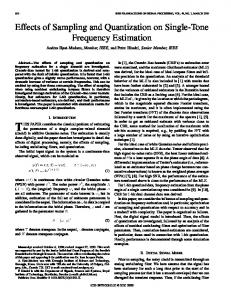
Another important consideration in the sampling process is to ensure that aliasing does not occur. Recall from theory that aliasing would occur whenever the sampling rate goes below twice the highest signal frequency, or whenever the signal frequency goes above the Nyquist rate (i.e., half of the sampling rate). To visualize the effect of aliasing in the sampling and reconstruction process, consider the signal plots shown in Fig. 3.11 below.

DSP Lab Manual – Ronald M. Pascual & FEU Institute of Technology

Page 40

Fig. 3.11. An illustration of the effect of aliasing in sampling process.

The solid blue curve in Fig. 3.11 represents a continuous-time or an analog periodic signal. The sequence of bubbles or sample markers represents the discrete-time sequence generated from the sampling process that uses a sampling rate which is below the Nyquist rate. Upon signal reconstruction or interpolation of the samples in the discrete-time signal, observe that a certain low-frequency signal, not equal to the original high-frequency signal, was reconstructed instead. This reconstructed signal is represented by the dotted red curve in Fig. 3.11.

Exercise 3.4 Type and run the script named ‘exer_3_4.m’ given below in Fig. 3.12. Upon running, the script should produce the output plots shown in Fig. 3.11.

QUESTION 3.4: What is the length of signal the signal ‘x’ in line 4 of ‘exer_3_4.m’?

DSP Lab Manual – Ronald M. Pascual & FEU Institute of Technology

Page 41

Fig. 3.12. The script ‘exer_3_4.m’ for Exercise 3.4.

QUESTION 3.5: What is the purpose of the command in line 6 of ‘exer_3_4.m’? How do the lengths of signals ‘x’ and ‘y’ compare?

QUESTION 3.6: What is the purpose of the command ‘interp’ in line 7 of ‘exer_3_4.m’? How do the lengths of signals ‘y’ and ‘z’ compare?

*** Machine Problem The Lab Instructor provides the machine problem for this chapter.

DSP Lab Manual – Ronald M. Pascual & FEU Institute of Technology

Page 42

MATLAB Code/Notes: _____________________________________________________________________________________ _____________________________________________________________________________________ _____________________________________________________________________________________ _____________________________________________________________________________________ _____________________________________________________________________________________ _____________________________________________________________________________________ _____________________________________________________________________________________ _____________________________________________________________________________________ _____________________________________________________________________________________ _____________________________________________________________________________________ _____________________________________________________________________________________ _____________________________________________________________________________________ _____________________________________________________________________________________ _____________________________________________________________________________________ _____________________________________________________________________________________ _____________________________________________________________________________________ _____________________________________________________________________________________ _____________________________________________________________________________________ _____________________________________________________________________________________ _____________________________________________________________________________________ _____________________________________________________________________________________ _____________________________________________________________________________________ _____________________________________________________________________________________ _____________________________________________________________________________________ _____________________________________________________________________________________ _____________________________________________________________________________________ _____________________________________________________________________________________ _____________________________________________________________________________________ _____________________________________________________________________________________ _____________________________________________________________________________________ _____________________________________________________________________________________ _____________________________________________________________________________________ _____________________________________________________________________________________ _____________________________________________________________________________________ _____________________________________________________________________________________ _____________________________________________________________________________________ _____________________________________________________________________________________ _____________________________________________________________________________________ _____________________________________________________________________________________ _____________________________________________________________________________________ DSP Lab Manual – Ronald M. Pascual & FEU Institute of Technology

Page 43

Results and Conclusion: _____________________________________________________________________________________ _____________________________________________________________________________________ _____________________________________________________________________________________ _____________________________________________________________________________________ _____________________________________________________________________________________ _____________________________________________________________________________________ _____________________________________________________________________________________ _____________________________________________________________________________________ _____________________________________________________________________________________ _____________________________________________________________________________________ _____________________________________________________________________________________ _____________________________________________________________________________________ _____________________________________________________________________________________ _____________________________________________________________________________________ _____________________________________________________________________________________ _____________________________________________________________________________________ _____________________________________________________________________________________ _____________________________________________________________________________________ _____________________________________________________________________________________ _____________________________________________________________________________________ _____________________________________________________________________________________ _____________________________________________________________________________________ _____________________________________________________________________________________ _____________________________________________________________________________________ _____________________________________________________________________________________ _____________________________________________________________________________________ _____________________________________________________________________________________ _____________________________________________________________________________________ _____________________________________________________________________________________ _____________________________________________________________________________________ _____________________________________________________________________________________ _____________________________________________________________________________________ _____________________________________________________________________________________ _____________________________________________________________________________________ _____________________________________________________________________________________ _____________________________________________________________________________________ _____________________________________________________________________________________ _____________________________________________________________________________________ _____________________________________________________________________________________ _____________________________________________________________________________________ DSP Lab Manual – Ronald M. Pascual & FEU Institute of Technology

Page 44