52nd IEEE Conference on Decision and Control December 10-13, 2013. Florence, Italy
Distributed Computation of Node and Edge Betweenness on Tree Graphs Wei Wang and Choon Yik Tang
Abstract— Knowing how important a node or an edge is, within a network, can be very valuable. In the area of complex networks, a variety of centrality measures, which assign to each node or edge a number representing its importance, have been proposed. In this paper, we consider two such measures, namely, node and edge betweenness that characterize how often a node or edge lies on the shortest paths between all pairs of nodes. For each measure, we use a dynamical systems approach to develop continuous- and discrete-time distributed algorithms, which enable every node in an undirected and unweighted tree graph to compute its own measure with only local interaction and without any centralized coordination. We show that the algorithms are simple and scalable, with the continuous-time version being unconditionally exponentially convergent, and the discrete-time version unconditionally exhibiting a deadbeat response. Moreover, we show that they require minimal node memories to execute, bypass entirely the need to construct shortest paths, and can handle time-varying topologies.
(a) Node betweenness. Fig. 1.
I. I NTRODUCTION In many applications of networks, nodes and edges within a network have different importance. Due to where they are located in the network, and who they are connected with, some nodes and edges are inherently more critical to the network’s well-being than others. Thus, knowing how important a node or an edge is, by itself or by its neighbors, can be very valuable, for instance, in identifying those who are susceptible/unattractive to malicious attacks, and those who are bottleneck/non-limiting to network performances, so that preventive measures may be taken and resources may be properly allocated. In the area of complex networks [1]–[6], a growing set of statistical measures referred to as centrality measures, which assign to each node or edge a number representing its importance, have been proposed. In this paper, we consider the distributed computation of two such measures, namely, node and edge betweenness. To facilitate the development, we define below each of these measures, which applies to an undirected, unweighted and connected graph G = (V, E), where V = {1, 2, . . . , N } denotes the set of N ≥ 2 nodes and E ⊂ {{i, j} : i, j ∈ V, i 6= j} denotes the set of edges: • The node betweenness Bi of a node i ∈ V is first conceptualized in [7] and later defined in [8] as Bi ,
X X σ(k, ℓ, i) , σ(k, ℓ)
•
Node and edge betweenness.
where σ(k, ℓ, i) is the number of shortest paths from nodes k to ℓ that go through node i, and σ(k, ℓ) is the number of shortest paths from nodes k to ℓ. Hence, Bi is the number of times node i lies on the shortest path between any pair of nodes k and ℓ. In the case where there are multiple shortest paths between nodes k and ℓ, the fraction of them that go through node i is counted. It follows that Bi attempts to measure how “strategically located” node i is within the graph G, making it one of the most fundamental centrality measures [9] that has found applications in such areas as power grids [10], transportation networks [11], [12], bioinformatics [13], and bibliometrics [14]. Figure 1(a) illustrates the notion of node betweenness, where the darker a node, the higher its betweenness. Observe that node betweenness can be quite different even among neighbors. Analogous to Bi , the edge betweenness B{i,j} of an edge {i, j} ∈ E is defined in [8] as X X σ(k, ℓ, {i, j}) , (2) B{i,j} , σ(k, ℓ) k∈V ℓ∈V ℓ6=k
where σ(k, ℓ, {i, j}) is the number of shortest paths from nodes k to ℓ that go through edge {i, j}. Like Bi , B{i,j} is the fraction of times edge {i, j} lies on the shortest paths between any pair of nodes k and ℓ. It therefore characterizes how strategically located edge {i, j} is within the graph G, which may represent, say, a road in a city, or a transmission line in a power grid. Figure 1(b) depicts the notion of edge betweenness, showing that it parallels that of node betweenness. Although node and edge betweenness are useful centrality measures, their computation may be difficult because they are defined in terms of all the shortest paths. While there are several well-established algorithms for computing shortest
(1)
k∈V ℓ∈V k6=i ℓ6=i,k
W. Wang and C. Y. Tang are with the School of Electrical and Computer Engineering, University of Oklahoma, Norman, OK 73019, USA (e-mail:
[email protected],
[email protected]). This work was supported by the National Science Foundation under grant CMMI-0900806.
978-1-4673-5717-3/13/$31.00 ©2013 IEEE
(b) Edge betweenness.
43
them, i.e., σ(k, ℓ) = 1. Thus, the node betweenness Bi of each node i ∈ V introduced in (1) simplifies to X X Bi = σ(k, ℓ, i). (3)
paths (e.g., the Floyd-Warshall algorithm [15] and Johnson’s algorithm [16]), and a few for computing betweenness (e.g., [17]–[19]), these algorithms are centralized in nature, requiring that all the information about the graph G be available at one place, at one time in order to execute. Such a requirement, unfortunately, is often difficult to meet especially in a large-scale network, due to security and privacy reasons and storage and single-point failure issues. Motivated by the aforementioned consideration and by successful development of a rich collection of distributed consensus/computation/optimization algorithms (e.g., [20]– [29], to name just a few), in this paper we consider the distributed computation of node and edge betweenness. We show that if the graph G is a tree, it is possible to construct continuous- and discrete-time distributed algorithms, which enable each node i ∈ V in the tree G to compute its own node betweenness Bi and its incident edge betweenness B{i,j} for every j ∈ Ni = {j ∈ V : {i, j} ∈ E}, with only local interaction and without any centralized coordination. In systems-theoretic terms, the algorithms are networked dynamical systems with affine state equations and nonlinear output equations, in which each node maintains a small subset of the state and output variables and updates them synchronously and homogeneously. We show that the algorithms each has a unique equilibrium point in the state space, at which the corresponding outputs are the unknown Bi ’s and B{i,j} ’s. Moreover, the unique equilibrium point for the continuous-time algorithm is unconditionally exponentially stable, with a convergence rate that is independent of the tree G (as measured by the eigenvalues of the system matrix). In contrast, the unique equilibrium point for the discrete-time algorithm is unconditionally finite-time stable, with the finite convergence time coinciding with the diameter of G (i.e., the system exhibits a deadbeat response). Finally, as can be seen from their development, the algorithms are simple and scalable, require minimal node memories to execute, bypass entirely the need to construct shortest paths, and can handle time-varying topologies (as long as G remains a tree). The outline of this paper is as follows: Section II derives a number of algebraic relationships that are key to subsequent development. Based on them, Section III designs and analyzes the continuous- and discrete-time distributed algorithms. Section IV presents simulation results that demonstrate the effectiveness of the algorithms. Finally, Section V concludes the paper and outlines possible future work. II. D ERIVATION
OF
k∈V ℓ∈V k6=i ℓ6=i,k
Moreover, since G is a tree, for each edge {i, j} ∈ E, deleting this edge results in two connected components, one containing node j and the other containing node i. For convenience, let V(i,j) and V(j,i) denote, respectively, the nodes in these two connected components, so that V(i,j) ∪ V(j,i) = V, j ∈ V(i,j) 6= ∅, and i ∈ V(j,i) 6= ∅. With this notation, for each node i ∈ V, the set V can be partitioned into {i} and V(i,j) ∀j ∈ Ni , where Ni = {j ∈ V : {i, j} ∈ E} denotes the set of neighbors of node i. It follows that (3) can be written as X X X X Bi = σ(k, ℓ, i). (4) k′ ∈Ni k∈V(i,k′ ) ℓ′ ∈Ni ℓ∈V(i,ℓ′ ) ℓ6=k
Again, due to G being a tree, ∀k ′ ∈ Ni and ∀ℓ′ ∈ Ni , if k ′ 6= ℓ′ , then ∀k ∈ V(i,k′ ) and ∀ℓ ∈ V(i,ℓ′ ) , we have σ(k, ℓ, i) = 1. Otherwise, i.e., if k ′ = ℓ′ , then ∀k ∈ V(i,k′ ) and ∀ℓ ∈ V(i,ℓ′ ) with k 6= ℓ, we have σ(k, ℓ, i) = 0. In other words, if k ′ and ℓ′ belong to different connected components when node i is deleted, then for any node k in the same connected component as node k ′ , and for any node ℓ in the same connected component as node ℓ′ , the shortest path joining nodes k and ℓ must go through node i. Otherwise, i.e., if k ′ and ℓ′ belong to the same connected component when node i is deleted, then the shortest path joining nodes k and ℓ does not go through node i. Therefore, (4) can be rewritten as X X X X Bi = 1 k′ ∈Ni k∈V(i,k′ ) ℓ′ ∈Ni ℓ∈V(i,ℓ′ ) ℓ′ 6=k′
=
X X
|V(i,k′ ) | · |V(i,ℓ′ ) |,
(5)
k′ ∈Ni ℓ′ ∈Ni ℓ′ 6=k′
where | · | denotes the cardinality of a set. Since the quantity |V(i,j) | is often referred to in this paper, for convenience let us denote it as x(i,j) , i.e., x(i,j) = |V(i,j) |.
(6)
With (6), the node betweenness Bi of each node i ∈ V in (5) becomes X X Bi = x(i,j) x(i,k) . (7)
K EY A LGEBRAIC E QUATIONS
Reconsider the undirected, unweighted and connected graph G = (V, E) in Section I and suppose G is a tree, i.e., it has N nodes in V and N − 1 edges in E with no cycles. Although G is undirected, for the purpose of development let us associate with each edge {i, j} ∈ E a pair of directed edges denoted as (i, j) and (j, i) (i.e., braces are for undirected edges, while parentheses are for directed ones), and let E˜ denote the set of 2(N − 1) directed edges. Observe that since G is a tree, for each pair of distinct nodes k, ℓ ∈ V, there is exactly one shortest path joining
j∈Ni k∈Ni k6=j
In the above paragraph, we have shown that the node betweenness Bi of each node i ∈ V, originally defined in (1) in terms of the shortest paths between all pairs of nodes, may be cast into a form (7) that does not involve any shortest path, but rather the number of nodes contained in each “branch” attached to node i, i.e., the x(i,j) ’s. As it turns out, the same may be carried out for the edge betweenness 44
B{i,j} of each edge {i, j} ∈ E defined in (2). To see this, recall that σ(k, ℓ) = 1 ∀k, ℓ ∈ V, k 6= ℓ. Hence, for each edge {i, j} ∈ E, the edge betweenness B{i,j} defined in (2) reduces to XX σ(k, ℓ, {i, j}). (8) B{i,j} = k∈V ℓ∈V ℓ6=k
To further simplify (8), notice that for each edge {i, j} ∈ E, the set V can be partitioned into V(i,j) and V(j,i) . Also note that if k ∈ V(i,j) and ℓ ∈ V(j,i) , or if ℓ ∈ V(i,j) and k ∈ V(j,i) , then σ(k, ℓ, {i, j}) = 1 since the shortest path joining nodes k and ℓ must go through edge {i, j}. Otherwise, i.e., if k, ℓ ∈ V(i,j) or k, ℓ ∈ V(j,i) , then σ(k, ℓ, {i, j}) = 0 since the shortest path joining nodes k and ℓ does not go through edge {i, j}. Thus, (8) can be restated as X X X X B{i,j} = 1+ 1 k∈V(i,j) ℓ∈V(j,i)
Fig. 2.
k∈V(j,i) ℓ∈V(i,j)
= 2x(i,j) x(j,i) ,
R2(N −1) obtained by stacking these 2(N − 1) unknowns x(i,j) ’s, (12) may be written in matrix form as
(9)
confirming that the edge betweenness B(i,j) of each edge {i, j} ∈ E can indeed be expressed as a function of x(i,j) and x(j,i) . As it follows from the nonlinear algebraic equations (7) and (9), if each node i ∈ V knows the value of x(i,j) ∀j ∈ Ni , then it could calculate Bi by itself. If, in addition, node i knows the value of x(j,i) ∀j ∈ Ni , then it could also calculate B{i,j} ∀j ∈ Ni . Therefore, if a method that allows every node i ∈ V to learn about the values of x(i,j) and x(j,i) ∀j ∈ Ni could be devised, the problem would be solved. Motivated by this observation, we next derive algebraic equations relating the 2(N − 1) unknowns x(i,j) ∀(i, j) ∈ E˜ (recall that E˜ is the set of 2(N − 1) directed edges). For each i ∈ V and each j ∈ Ni , due to (6) and to the fact that V(i,j) ∪ V(j,i) = V and V(i,j) ∩ V(j,i) = ∅, we have x(i,j) + x(j,i) = N,
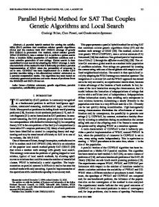
A graphical illustration of expression (12).
∀i ∈ V, ∀j ∈ Ni .
Hx = 1,
where H ∈ R2(N −1)×2(N −1) is a square matrix and 1 ∈ R2(N −1) is the all-one column vector. The following lemma and corollary show that the matrix H has appealing properties: Lemma 1. The matrix H is a unipotent matrix with all its 2(N − 1) eigenvalues at 1. Proof. Observe that H in (13) depends on the order in which the 2(N − 1) variables x(i,j) ’s are stacked into the vector x. Also note that such an order does not affect the eigenvalues of H because permutation of rows and columns of H may be regarded as a similarity transformation that leaves all the eigenvalues of H intact. Hence, consider without loss of generality the following rule for stacking the 2(N − 1) variables x(i,j) ’s: First, arbitrarily pick a node r ∈ V and view it as a root node. Second, let L0 denote the set containing only node r. Also, let L1 ⊂ V denote the set of nodes that are one hop away from node r, L2 ⊂ V the set of nodes that are two hops away, and so on, until the set Lp is reached, where p = maxj∈V drj and drj is the distance between nodes r and j. Starting with an empty vector x, insert into x the set of x(i,j) where i ∈ L0 and j ∈ L1 , where the order among them can be arbitrary. Upon completion, insert into x the set of x(i,j) where i ∈ L1 and j ∈ L2 . Repeat this process until x(i,j) for all i ∈ Lp−1 and j ∈ Lp are inserted. At this point, the first N − 1 elements of the vector x are defined, making up half of its length of 2(N − 1). Third, for each ℓ ∈ {1, 2, . . . , N − 1}, if the ℓth element of x is x(i,j) , then let the (ℓ + N − 1)th element of x be x(j,i) . In this fashion, the order in which the 2(N − 1) variables x(i,j) ’s are stacked into the vector x is completely defined. With this ordering, it is straightforward to see that
(10)
Likewise, for each j ∈ V, due again to (6) and to the sets {j} and V(j,k) ∀k ∈ Nj forming a partition of V, we have X x(j,k) = N − 1, ∀j ∈ V. (11) k∈Nj
Combining (10) and (11), we obtain X x(i,j) − x(j,k) = 1, ∀i ∈ V, ∀j ∈ Ni .
(13)
(12)
k∈Nj k6=i
Expression (12) has a couple of implications. First, as is illustrated in Figure 2, expression (12) implies that if edge {i, j} ∈ E is removed from the tree G, the number of nodes in the connected component containing node j (i.e., x(i,j) ) is equal to one (i.e., due to node j) plus the remaining number of nodesP in that connected component, which happens to be equal to k∈Nj ,k6=i x(j,k) . Second, expression (12) provides 2(N − 1) linear equations relating the 2(N − 1) unknowns ˜ i.e., there are as many equations as there x(i,j) ∀(i, j) ∈ E, are unknowns. Consequently, by introducing a vector x ∈ 45
H has the form 1 ∗ 0 1 .. . . . . 0 ... H= 0 ∗ ∗ 0 . . .. .. ∗ ...
... .. . .. . 0 ... .. . ..
. ∗
∗ 0 .. . 0 . ∗ .. 1 0 ∗ 1 .. . ∗ . ∗ .. 0 ∗
0
...
0
0 .. .
... .. . ... ... .. .
0 .. .
0 0 1 .. . ...
..
. ∗
0 0 .. . 0 1
(9), and (15) collectively suggest the following synchronous and homogeneous rule for updating all the estimates: X xˆ˙ (i,j) (t) = −ˆ x(i,j) (t)+ x ˆ(j,k) (t)+1, ∀i ∈ V, ∀j ∈ Ni ,
.
k∈Nj k6=i
(16a)
(14)
ˆi (t) = B
ˆ{i,j} (t) = 2ˆ B x(i,j) (t)ˆ x(j,i) (t),
∀i ∈ V,
(16b)
∀i ∈ V, ∀j ∈ Ni . (16c)
Notice that (16a) is equivalent to (15), while (16b) and (16c) are based on (7) and (9). Hence, algorithm (16) may be viewed as a networked dynamical system with an affine state equation and a nonlinear output equation. Also note that to implement algorithm (16), every pair of one-hop neighbors i, j ∈ V with {i, j} ∈ E need to continuously exchange their x ˆ(i,j) (t) and x ˆ(j,i) (t). There are, however, no restrictions on the initial condition, no needs to construct shortest paths, and no algorithm parameters to tune. The following theorem summarizes the above findings:
Corollary 1. The matrix I − H, where I ∈ R2(N −1)×2(N −1) is the identity matrix, is a nilpotent matrix with all its 2(N − 1) eigenvalues at 0.
Theorem 1. The continuous-time algorithm (16) has a unique equilibrium point x that is exponentially sta˜ we have ble, such that for any x ˆ(i,j) (0) ∀(i, j) ∈ E, ˜ limt→∞ x ˆ(i,j) (t) = x(i,j) ∀(i, j) ∈ E. In addition, ˆ{i,j} (t) = B{i,j} ˆi (t) = Bi ∀i ∈ V and limt→∞ B limt→∞ B ∀{i, j} ∈ E.
Proof. The proof is an immediate consequence of (14). A NALYSIS OF D ISTRIBUTED A LGORITHMS
AND
In this section, we leverage the results from Section II to develop a continuous-time and a discrete-time distributed algorithm for computing node and edge betweenness.
B. Discrete-Time Distributed Algorithm
A. Continuous-Time Distributed Algorithm
The continuous-time algorithm (16) is made possible by the unipotent property of H established in Lemma 1. In what follows, we make use of the nilpotent property of I − H from Corollary 1 to design its discrete-time counterpart. To this end, notice that if we form a difference equation
Recall from Section II that if each node i ∈ V is able to determine the values of x(i,j) and x(j,i) ∀j ∈ Ni , then it could use (7) and (9) to compute Bi and B{i,j} ∀j ∈ Ni by itself. Also, recall from (13) that the 2(N − 1) variables x(i,j) ∀(i, j) ∈ E˜ are linearly related through H, which by Lemma 1 is unipotent with all its eigenvalues at 1. This result implies that the 2(N − 1) linear equations (12) relating the x(i,j) ’s are independent and, thus, have a unique solution. More importantly, the result implies that −H is always asymptotically stable with all its eigenvalues at −1 regardless of the topology of the tree G. These two implications, together, say that if we form a differential equation ˆ˙ (t) = −H x ˆ (t) + 1, x
x ˆ(i,j) (t)ˆ x(i,k) (t),
j∈Ni k∈Ni k6=j
Notice from (14) that H has a 2-by-2 block triangular structure, in which the first block on the diagonal of H is an upper triangular matrix with 1 on its diagonal, while the second block is a lower triangular matrix also with 1 on its diagonal. Thus, all the 2(N − 1) eigenvalues of H are at 1, making it unipotent and completing the proof.
III. D ESIGN
X X
ˆ (t + 1) = (I − H)ˆ x x(t) + 1,
(17)
where t ∈ {0, 1, 2, . . .} here denotes discrete time and ˆ (t) ∈ R2(N −1) plays the same role as before, then because x ˆ (t) of (13) and because all the eigenvalues of I − H are 0, x would converge to the unique equilibrium point x in finite ˆ (0). Hence, (17) time irrespective of the initial condition x suggests the following discrete-time distributed algorithm for ˆi (t)’s, and B{i,j} ’s: iterating the estimates xˆ(i,j) (t)’s, B X x ˆ(i,j) (t + 1) = x ˆ(j,k) (t)+1, ∀i ∈ V, ∀j ∈ Ni , (18a)
(15)
ˆ (t) ∈ where t ∈ [0, ∞) denotes continuous time and x R2(N −1) is an estimate of the unknown x at time t, then ˆ (0), the estimate x ˆ (t) would expofor any initial condition x nentially converge to the unique equilibrium point x with a convergence rate characterized by the uniform eigenvalues of −1. Therefore, we may define a continuous-time distributed ˜ algorithm as follows: for each directed edge (i, j) ∈ E, let xˆ(i,j) (t) ∈ R represent an estimate of x(i,j) at time t and suppose xˆ(i,j) (t) is maintained in node i’s memory. In addition to maintaining xˆ(i,j) (t) ∀j ∈ Ni , suppose each ˆi (t) ∈ R of Bi and an node i ∈ V maintains an estimate B ˆ{i,j} (t) ∈ R of B{i,j} ∀j ∈ Ni . Equations (7), estimate B
k∈Nj k6=i
ˆi (t) = B
X X
x ˆ(i,j) (t)ˆ x(i,k) (t),
∀i ∈ V, (18b)
j∈Ni k∈Ni k6=j
ˆ{i,j} (t) = 2ˆ B x(i,j) (t)ˆ x(j,i) (t),
∀i ∈ V, ∀j ∈ Ni . (18c)
Note that, similar to its continuous-time counterpart, algorithm (18) consists of an affine state equation and a nonlinear output equation. In fact, (18b) and (18c) are identical to (16b) and (16c), except that t here is integer-valued. Furthermore, as is asserted in the theorem below, algorithm (18) not only 46
Node 2 0 10 18 Node 3 16 10 10 0 8 0 Node 5 Node 6 Node 4
Node 1 Node 2 0 0 10 Node 3 14 10 18 10 14 10 0 0 Node 5 Node 6 Node 4
Node 1 Node 2 8 0 16 Node 3 12 10 10 18 14 10 0 0 Node 5 Node 6 Node 4
(a) Over t ∈ [0, 10].
(b) Over t ∈ [10, 20].
(c) Over t ∈ [20, 30].
Node 1 0 10
20 18 16 14 12 ˆi (t)’s B
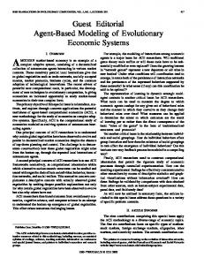
Fig. 3. A 6-node tree graph and its node and edge betweenness over time t ∈ [0, 30].
10 8 6
achieves a deadbeat response, it does so in t = D(G) time steps, where D(G) is the diameter of the tree G:
ˆ1 B ˆ2 B ˆ3 B ˆ4 B ˆ5 B ˆ6 B
4 2
Theorem 2. The discrete-time algorithm (18) has a unique equilibrium point x that is finite-time stable, such that for any x ˆ(i,j) (0) ∀(i, j) ∈ E˜ and for any t ∈ {D(G), D(G) + ˜ 1, D(G) + 2, . . .}, we have x ˆ(i,j) (t) = x(i,j) ∀(i, j) ∈ E, ˆ ˆ Bi (t) = Bi ∀i ∈ V, and B{i,j} (t) = B{i,j} ∀{i, j} ∈ E.
0 −2 0
5
10
15 Time t
20
25
30
(a) Node betweenness estimates. 20
Proof. Due to space limitation, the proof is omitted. IV. S IMULATION R ESULTS
16
In this section, we present two sets of simulation results that demonstrate the effectiveness of the continuous- and discrete-time algorithms.
ˆ{3,5} B
ˆ{3,5} B
18
ˆ{1,3} B
ˆ{3,5} B
ˆ{i,j} (t)’s B
14
A. Simulation of the Continuous-Time Distributed Algorithm Consider a tree graph with N = 6 nodes, whose topology changes from time to time, as shown in Figure 3. Specifically, Figure 3(a) shows the tree topology over time t ∈ [0, 10] and the resulting node and edge betweenness Bi ’s and B{i,j} ’s calculated using (1) and (2), while Figures 3(b) and 3(c) do the same for t ∈ [10, 20] and t ∈ [20, 30], respectively. As indicated by the arrows and dotted lines in Figures 3(b) and 3(c), edge {2, 3} is deleted and replaced by edge {2, 5} at time t = 10, while edge {3, 4} is deleted and replaced by edge {1, 4} at time t = 20, but the graph remains a tree. Suppose the nodes employ the continuous-time algorithm (16) to help them cooperatively compute their estimates ˆi (t)’s and B ˆ{i,j} (t)’s of the changing Bi ’s and B{i,j} ’s. B Figure 4 displays the simulation result. Observe that despite the time-varying topology, algorithm (16) allows the ˆi (t)’s and B ˆ{i,j} (t)’s to asymptotically track the nodes’ B Bi ’s and B{i,j} ’s without having to “restart” or “refresh”— an action that would likely be required if the algorithm were based on explicit shortest path construction. Indeed, the nodes may not even be aware, and are not required to notify or be notified, that the topology has changed. Also note that because of the time-varying topology, B{2,3} is defined only for t ∈ [0, 10], B{2,5} for t ∈ [10, 30], B{3,4} for t ∈ [0, 20], and B{1,4} for t ∈ [20, 30]—and so are their ˆ{i,j} (t)’s. estimates B
12 10
ˆ{3,4} B
8 6
ˆ{5,6} B
ˆ{1,3} , B ˆ{2,3} B ˆ{1,3} B
ˆ{3,4} B
ˆ{2,5} B ˆ{1,4} B
ˆ{2,5} B
ˆ{5,6} B
ˆ{5,6} B
4 2 0 0
5
10
15 Time t
20
25
30
(b) Edge betweenness estimates. Fig. 4. Performance of the continuous-time algorithm (16) in computing node and edge betweenness on the time-varying 6-node tree graph.
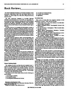
nodes 7 and 16). Suppose the nodes utilize the discreteˆi (t)’s time algorithm (18) to jointly compute their estimates B ˆ and B{i,j} (t)’s of the Bi ’s and B{i,j} ’s. Figure 6 shows the simulation result, where it can be seen that algorithm (18) indeed exhibits a deadbeat response, allowing all the nodes’ ˆi (t)’s and B ˆ{i,j} (t)’s to reach the Bi ’s and B{i,j} ’s in finite B time of no more than t = 11 time steps. V. C ONCLUSION
AND
F UTURE W ORK
In this paper, we have introduced a set of continuous- and discrete-time distributed algorithms, which enable nodes in a tree graph to cooperatively compute their individual node betweenness and incident edge betweenness. Constructed using a dynamical systems approach, we have shown that the algorithms possess several positive attributes, such as being simple, scalable, and exponentially or finite-time stable with strong convergence characteristics, and being applicable to time-varying tree graphs. Given that trees are a very special type of graphs, possible future research includes developing distributed algorithms
B. Simulation of the Discrete-Time Distributed Algorithm Consider a tree graph with N = 16 nodes as shown in Figure 5, in which Figure 5(a) displays the node indices and Figure 5(b) displays the corresponding node and edge betweenness Bi ’s and B{i,j} ’s. Notice that the diameter of this tree graph is 11 (attained by the shortest path between 47
14
4
15
3
2
16
6
1
7 13 8 12
9 11
10
(a) Node indices.
0 30 94 78 52 56 110 28 30 28 56 132 128 30 112 0 126 108 0 120 30 108 30 28 0 96 56 52 78 72
250
ˆ1 B ˆ2 B ˆ3 B ˆ4 B ˆ5 B ˆ6 B ˆ7 B ˆ8 B ˆ9 B ˆ10 B ˆ11 B ˆ12 B ˆ13 B ˆ14 B ˆ15 B ˆ16 B
0
200
150 ˆi (t)’s B
5
(b) Node and edge betweenness.
100
Fig. 5. A 16-node tree graph and its node indices and node and edge betweenness.
50
for computing betweenness and other centrality measures on general graphs, building perhaps on the ideas of this paper.
0 0
5
10 Time t
15
(a) Node betweenness estimates.
R EFERENCES [1] D. Watts and S. Strogatz, “The small world problem,” Collective Dynamics of Small-World Networks, vol. 393, pp. 440–442, 1998. [2] A. L. Barabasi and R. Albert, “Emergence of scaling in random networks,” Science, vol. 286, no. 5439, pp. 509–512, 1999. [3] L. A. Adamic, R. M. Lukose, A. R. Puniyani, and B. A. Huberman, “Search in power-law networks,” Physical Review E, vol. 64, no. 4, p. 046135, 2001. [4] B. Bollobas, Random graphs. New York, NY: Cambridge University Press, 2001, vol. 73. [5] R. Albert and A. Barabasi, “Statistical mechanics of complex networks,” Reviews of Modern Physics, vol. 74, no. 1, p. 47, 2002. [6] M. E. J. Newman, “The structure and function of complex networks,” SIAM Review, vol. 45, no. 2, pp. 167–256, 2003. [7] J. M. Anthonisse, “The rush in a directed graph,” Stiching Mathematisch Centrum Afdeling Mathematische Besliskunde, 1971. [8] L. C. Freeman, “A set of measures of centrality based on betweenness,” Sociometry, vol. 40, no. 1, pp. 35–41, 1977. [9] M. E. J. Newman, Networks: An Introduction. New York, NY: Oxford University Press, 2010. [10] S. Jin, Z. Huang, Y. Chen, D. G. Chavarria-Miranda, J. Feo, and P. C. Wong, “A novel application of parallel betweenness centrality to power grid contingency analysis,” in Proc. IEEE International Parallel and Distributed Processing Symposium, Atlanta, GA, 2010, pp. 1–7. [11] S. Lammer, B. Gehlsen, and D. Helbing, “Scaling laws in the spatial structure of urban road networks,” Physica A: Statistical Mechanics and Its Applications, vol. 363, no. 1, pp. 89–95, 2006. [12] P. Holme, “Congestion and centrality in traffic flow on complex networks,” Advances in Complex Systems, vol. 6, no. 2, pp. 163–176, 2003. [13] A. D. Sol, H. Fujihashi, and P. O. Meara, “Topology of smallworld networks of protein-protein complex structures,” Bioinformatics, vol. 21, no. 8, pp. 1311–1315, 2005. [14] L. Leydesdorff, “Betweenness centrality as an indicator of the interdisciplinarity of scientific journals,” Journal of the American Society for Information Science and Technology, vol. 58, no. 9, pp. 1303–1309, 2009. [15] R. W. Floyd, “Algorithm 97: Shortest path,” Communications of the ACM, vol. 5, no. 6, p. 345, 1962. [16] D. B. Johnson, “A note on Dijkstra’s shortest path algorithm,” Journal of the ACM, vol. 20, no. 3, pp. 385–388, 1973. [17] L. C. Freeman, S. P. Borgatti, and D. R. White, “Centrality in valued graphs: A measure of betweenness based on network flow,” Social Networks, vol. 13, no. 2, pp. 141–154, 1991. [18] U. Brandes, “A faster algorithm for betweenness centrality,” Journal of Mathematical Sociology, vol. 25, no. 2, pp. 163–177, 2001. [19] E. D. Kolaczyk, D. B. Chua, and M. Barthelemy, “Group betweenness and co-betweenness: Inter-related notions of coalition centrality,” Social Networks, vol. 31, no. 3, pp. 190–203, 2009. [20] J. N. Tsitsiklis, “Problems in decentralized decision making and computation,” Ph.D. Thesis, Massachusetts Institute of Technology, Cambridge, MA, 1984. [21] R. Olfati-Saber and R. M. Murray, “Consensus problems in networks of agents with switching topology and time-delays,” IEEE Transactions on Automatic Control, vol. 49, no. 9, pp. 1520–1533, 2004.
300
ˆ{1,2} B ˆ{2,3} B ˆ{3,4} B ˆ{3,6} B ˆ{4,5} B ˆ{4,14} B ˆ{6,7} B ˆ{7,8} B ˆ{8,9} B ˆ{8,10} B ˆ{10,11} B ˆ{11,12} B ˆ{12,13} B ˆ{14,15} B ˆ{15,16} B
250
ˆ{i,j} (t)’s B
200
150
100
50
0 0
5
10 Time t
15
(b) Edge betweenness estimates. Fig. 6. Performance of the discrete-time algorithm (18) in computing node and edge betweenness on the 16-node tree graph.
[22] W. Ren and R. W. Beard, “Consensus seeking in multiagent systems under dynamically changing interaction topologies,” IEEE Transactions on Automatic Control, vol. 50, no. 5, pp. 655–661, 2005. [23] S. Boyd, A. Ghosh, B. Prabhakar, and D. Shah, “Randomized gossip algorithms,” IEEE Transactions on Information Theory, vol. 52, no. 6, pp. 2508–2530, 2006. [24] W. Ren and R. Beard, Distributed Consensus in Multi-Vehicle Cooperative Control. New York, NY: Springer, 2008. [25] A. Olshevsky and J. N. Tsitsiklis, “On the nonexistence of quadratic Lyapunov functions for consensus algorithms,” IEEE Transactions on Automatic Control, vol. 53, no. 11, pp. 2642–2645, 2008. [26] A. Nedi´c, A. Ozdaglar, and P. A. Parrilo, “Constrained consensus and optimization in multi-agent networks,” IEEE Transactions on Automatic Control, vol. 55, no. 4, pp. 922–938, 2010. [27] J. Wang and N. Elia, “A control perspective for centralized and distributed convex optimization,” in Proc. IEEE Conference on Decision and Control and European Control Conference, Orlando, FL, 2011, pp. 3800–3805. [28] M. Zhu and S. Mart´ınez, “On distributed convex optimization under inequality and equality constraints,” IEEE Transactions on Automatic Control, vol. 57, no. 1, pp. 151–164, 2012. [29] J. Lu and C. Y. Tang, “Zero-gradient-sum algorithms for distributed convex optimization: The continuous-time case,” IEEE Transactions on Automatic Control, vol. 57, no. 9, pp. 2348–2354, 2012.
48