Distributed Selfish Replication. â. Nikolaos Laoutaris, Orestis Telelis, Vassilios Zissimopoulos, Ioannis Stavrakakis. Abstract. A commonly employed abstraction ...
Distributed Selfish Replication∗ Nikolaos Laoutaris, Orestis Telelis, Vassilios Zissimopoulos, Ioannis Stavrakakis
Abstract A commonly employed abstraction for studying the object placement problem for the purpose of Internet content distribution is that of a distributed replication group. In this work the initial model of distributed replication group of Leff, Wolf, and Yu (IEEE TPDS ’93) is extended to the case that individual nodes act selfishly, i.e., cater to the optimization of their individual local utilities. Our main contribution is the derivation of equilibrium object placement strategies that: (a) can guarantee improved local utilities for all nodes concurrently as compared to the corresponding local utilities under greedy local object placement; (b) do not suffer from potential mistreatment problems, inherent to centralized strategies that aim at optimizing the social utility; (c) do not require the existence of complete information at all nodes. We develop a baseline computationally efficient algorithm for obtaining the aforementioned equilibrium strategies and then extend it to improve its performance with respect to fairness. Both algorithms are realizable in practice through a distributed protocol that requires only limited exchange of information.
1
Introduction
Recent efforts to improve the service that is offered to Internet users have considered supplementing the traditional bandwidth-centric Internet with a rather non-traditional network resource – storage. A network node installs storage to replicate popular Internet content locally, and then provide it to local users and others efficiently (i.e., at a small end-to-end ∗
The authors are with the Department of Informatics and Telecommunications, University of Athens, 15784
Athens, Greece. Email: {laoutaris, telelis, vassilis, istavrak}@di.uoa.gr.
1
delay) and economically (i.e., without having to access the origin servers each time, thereby consuming bandwidth). Several technologies have been developed for this purpose, such as web caching, web mirroring, content distribution networks (CDNs), and lately peer-to-peer applications (P2P). A commonly employed abstraction for studying such systems is that of a distributed replication group [1]. Under this abstraction, nodes utilize their storage capacity to replicate information objects and make them available to local and remote users. Replication amounts to maintaining fixed copies of objects which, contrary to caching, cannot be removed before the re-invocation of the placement algorithm (caching amounts to storing temporary copies of objects upon request and then releasing them through a replacement algorithm in order to free storage for newer ones). A user’s request is first received by the local node. If the requested object is stored locally, it is returned to the requesting user immediately, thereby incurring a minimal access cost. Otherwise, the requested object is searched and fetched from other nodes of the group, at a potentially higher access cost. If the object cannot be located anywhere in the group, it is retrieved from an origin server, which is assumed to be laying outside the group (maximum access cost). Depending on the particular application, the search for objects at remote nodes may be conducted through query protocols [2], succinct summaries [3], DNS redirection [4] or distributed hash tables [5]. Several placement problems can be defined regarding a distributed replication group. The proxy (or cache, or mirror, or surrogate) placement problem refers to the selection of appropriate physical network locations (routers or AS’s) for installing content proxies [6, 7, 8, 9]. Another relevant problem is the object placement problem, which refers to the selection of objects for the nodes, under given node locations and capacities [1, 10, 11, 12, 13, 14]. Joint formulations of the above mentioned problems have also appeared, e.g., in [15, 16], where the proxy placement, proxy dimensioning, and object placement problems are combined into a single problem. All the aforementioned work has focused on the optimization of the so called social utility (sum of the individual local utilities of the nodes, defined as the delay and bandwidth gains from employing replication). Optimizing the social utility is naturally the objective in environments where a central authority dictates its replication decisions to the nodes. It
2
suits well applications such as web mirroring and CDNs, which are operated centrally by a single authority (this being the content creator or the content distributor). Applications that are run by multiple authorities, such as web caching networks and P2P networks, may also seek to optimize the social utility. This, however, requires some nodes to act in a spirit of voluntaryism, as the optimization of the social utility is often harmful to several local utilities. Consider as an example a group of nodes that collectively replicate content. If one of the nodes generates the majority of the requests, then a socially optimal (SO) object placement strategy will use the storage capacity of other nodes to replicate objects that do not fit in the over-active node’s storage space. Consequently, the users of these other nodes will experience a service deterioration as a result of their storage being hijacked by potentially irrelevant objects with regard to their local demand. In fact, such nodes would be better served if they acted independently and employed a greedy local (GL) object placement strategy (i.e., replicated the most popular objects according to the local demand). A similar situation can arise if caching, rather than replication, is in place: remote hits originating from other nodes may evict objects of local interest in an LRU-operated cache that participates in a web caching network (we study this problem in [17]). Concern for such exploitation can prevent rational nodes from participating in such groups, and, instead, lead them to operating in isolation in a greedy local manner. Such a behavior, however, is far from being desirable. Being GL is often ineffective in terms of performance, not only with respect to the social utility, but with respect to the individual local utilities too. For example, when the nodes have similar demand patterns and the inter-node distances are small, then replicating multiple times the same most popular objects, as done by the same repeated GL placement at all the nodes, is highly ineffective. Clearly, all the nodes may gain substantially in this case, if they cooperate and replicate different objects. In fact, it is even possible that an appropriate cooperation of the nodes can lead to a simultaneous improvement of all local utilities as compared to the GL performance. However, nodes cannot recognize such opportunities for mutually beneficial cooperation, since they are generally unaware of the remote demand patterns. On the other hand, they cannot know the impact (bad or good) that the SO object placement strategy may have on their own local utility. To address the above mentioned deadlock, we use as reference the object replication prob-
3
lem defined by Leff et al. [1], and extend it to account for the existence of selfishly motivated nodes. We use a strategic game in normal form [18] to model the contention between the selfish nodes and set out to identify pure Nash equilibrium object placement strategies (henceforth abbreviated EQ). There are several advantages in employing EQ strategies. First, by their definition, they can guarantee for each and every node of the group that its local utility under EQ will be at least as good as under GL, and possibly better. The first case (“at least as good”) precludes mistreatment problems such as those that can arise under the SO placement which cause the nodes to leave the group in pursuit of GL placement. The second case (“possibly better”) is the typical one, and points to the fact that implicit cooperation is induced even by selfishly behaving nodes as they attempt to do better than GL. Consequently, the EQ strategy is in position to break the above mentioned deadlock, as it forbids the mistreatment of any one node, while it also guards against the disintegration of the group, and the poor performance associated with the GL strategy. Our main result is that such EQ object placement strategies can be obtained by simple distributed algorithms that do not require the existence of complete information at all the nodes. We describe a two-step local search (TSLS) algorithm for this purpose. TSLS requires each node to know only its local demand pattern and the objects selected for replication by remote nodes, but not the remote demand patterns of other nodes (the demand pattern of a node defines explicitly its utility function, thus in the presented framework it is not assumed that nodes know the utility functions of other nodes). Knowing the remote demand patterns requires the transmission of too much information and thus is seldom possible in large distributed replication groups. On the other hand, knowing the objects selected for replication by remote nodes requires the exchange of much less information, which can be reduced further by employing simple encoding schemes such as Bloom filters [19] (see also [20, 21] for real distributed applications/protocols that utilize such information). Thus in terms of the required information, the proposed EQ strategies fit between the GL strategy that requires only local information, and the SO strategy that requires complete information. The TSLS algorithm employs the logical ordering of the nodes as a device for obtaining EQ in a simple and distributed manner. The ordering, however, can give some nodes an advantage which, sometimes, is difficult to justify, e.g., in the case of nodes that are identical,
4
hence lack any kind of difference in “merit” based on which a preferential treatment can be justified. To address such issues we develop the TSLS(k) algorithm, a constrained version of the baseline TSLS, which diminishes any advantage that a node may have over other nodes due to its particular turn in the execution of the algorithm. We implement both algorithms through a common protocol that requires the exchange of a limited amount of information and, thus, is rather simple to apply. The remainder of the article is structured as follows. Section 2 describes formally the distributed replication group and the distributed selfish replication (DSR) game. Section 3 describes the baseline TSLS object placement algorithm. Section 4 establishes that the TSLS algorithm produces a pure Nash equilibrium object placement strategy for the DSR game. Section 5 includes a discussion concerning the need for node ordering as well as its implications on the individual gains of the nodes. Section 6 is devoted to the presentation of the TSLS(k) algorithm. Section 7 describes a common protocol for implementing the two algorithms. Section 8 demonstrates some numerical examples for highlighting the operation of the algorithms and the properties of the various placements. Section 9 reviews related game theoretic approaches to replication and caching. Finally, Section 10 concludes the article and points to some interesting problems for future work.
2
Definitions
Let oi , 1 ≤ i ≤ N , and vj , 1 ≤ j ≤ n, denote the ith unit-sized object and the jth node, and let O = {o1 , . . . , oN } and V = {v1 , . . . , vn } denote the corresponding sets. Node vj is assumed to have a storage capacity for Cj unit-sized objects and a demand described by a rate vector rj over O, rj = {r1j , . . . , rN j }, where rij denotes the rate (requests per second) at which node � vj requests object oi ; let also ρj = oi ∈O rij denote the total request rate from vj . We follow the access cost model defined in [1] and later used in several works, including [10, 22, 23]. Under this model, accessing an object from a node’s local cache costs tl , from a remote node’s cache tr , and from the origin server ts , with tl ≤ tr ≤ ts (Fig. 1 depicts the envisaged distributed replication group). Such a definition of cost, in addition to allowing for a much clearer analysis of the dynamics of selfish replication, has also a strong relevance to practice.
5
This is because distributed replication groups, like the ones studied here, become meaningful when there is a high degree of proximity among the nodes, while the corresponding distances to reach the origin servers are far too larger. Such is, for example, the case of nodes belonging to the same organization or autonomous system. In such environments, the inter-node distances may be considered to be approximately equal to an average value tr , when compared to the much larger distance to the remote servers. On the other hand, it is clear that when the inter-node distances for each pair of nodes vary significantly, possibly approaching ts , then it becomes less meaningful to seek an efficient cooperation between such distant nodes. Let Rj = {oi ∈ O : rij > 0} denote the request set of node vj . Let Pj denote the placement of node vj , that is the set of objects replicated at this node; Pj ⊆ O and |Pj | = Cj (in principle it can be |Pj | ≤ Cj if, for example, less than Cj objects have none zero request rate, but we can safely assume that each node takes full advantage of its capacity by also replicating zerorated objects arbitrarily, until |Pj | = Cj ). Let P = {P1 , P2 , . . . , Pn } be referred to as a global placement and let P−j = P1 ∪ . . . ∪ Pj−1 ∪ Pj+1 ∪ . . . ∪ Pn denote the set of objects collectively held by nodes other than vj under the global placement P . The gain for node vj under P is defined as follows: Gj (P ) =
�
rij · (ts − tl ) +
oi ∈Pj
�
rij · (ts − tr )
(1)
oi ∈P / j oi ∈P−j
This definition of gain considers all the objects that exist somewhere in the group under the global placement P , and returns a weighted summation of vj ’s local request rate for each one of them, and the distance spared by having vj accessing them from the closest position in the group (either locally, or from a remote node) and thus avoiding going to the origin server, which is assumed to be the furthest away. Notice that we model only the “read” operations from the users. We could possibly include “write” operations in the same setting but this is not required by our targeted application which is the dissemination of large electronic content (audio files, movies, software distributions). Such content is rarely altered. On the other hand, web-pages are regularly updated, but such content should probably be investigated under a different setting, one without storage capacity constraints as the ones considered here (the small size of typical web-pages in conjunction with the large capacity of hard disk drives allows for assuming the existence of “infinite storage” at content nodes for web content [16]).
6
OS
tr
Step 0 (initialization): Pj0 = Greedyj (∅), 1 ≤ j ≤ n.
ts
−
1 ), 1 ≤ j ≤ n, Step 1 (improvement): Pj1 = Greedyj (P−j −
1 1 0 where, P−j = P11 ∪ . . . ∪ Pj−1 ∪ Pj+1 ∪ . . . ∪ Pn0
vj rij Figure 1:
Table 1:
A distributed replication group.
The TSLS algorithm.
In the sequel, we define a game that captures the dynamics of distributed object replication under selfishly behaving nodes. Definition 1 (DSR game) The distributed selfish replication game is defined by the tuple �V, {Pj }, {Gj }�, where: • V is the set of n players, which in this case are the nodes. • {Pj } is the set of strategies available to player vj . As the strategies correspond to place� � ments, player vj has CNj possible strategies. • {Gj } is the set of utilities for the individual players. The utility of player vj under the outcome P , which in this case is a global placement, is Gj (P ). DSR is a n-player, non-cooperative, non-zerosum game [18]. For this game, we seek equilibrium strategies, and in particular, pure Nash equilibrium strategies. Definition 2 (pure Nash equilibrium for DSR) A pure Nash equilibrium for DSR is a global ∗ ∗ , Pj , Pj+1 , . . . , Pn∗ )), placement P ∗ , such that for every node vj ∈ V , Gj (P ∗ ) ≥ Gj ((P1∗ , . . . , Pj−1
for all Pj ∈ {Pj }. That is, under such a placement P ∗ , nodes cannot modify their individual placements unilaterally and benefit. In the sequel, we develop polynomial time algorithms that, given an instance of the DSR game, can produce several Nash equilibrium placement strategies for it.
7
3
A two-step local search algorithm
In this section we present a two-step local search algorithm (TSLS) that computes a placement for each one of the nodes. In Section 4 we show that these placements correspond to a Nash equilibrium global placement, that is they are EQ strategies. In Section 6, we modify the two-step local search algorithm in order to overcome some of its limitations. Let Pj0 and Pj1 denote the GL placement strategy and the placement strategy identified by TSLS for node vj , respectively. Let also Greedyj (P) denote a function that computes the optimal placement for node vj , given the set P of distinct objects collectively held by other nodes; we elaborate on this function later on in the section. Table 1 outlines the proposed TSLS algorithm. At the initialization step (Step 0) nodes compute their GL placements Pj0 . This is done by evaluating Greedyj (∅) for each vj , capturing the case in which nodes operate in isolation (P = ∅). At the improvement step (Step 1) nodes observe the placements of other nodes and, based on this information, proceed to improve their own. The order in which nodes take turn in improving their initial placements is determined based on their ids (increasing order). Thus at vj ’s turn to improve its initial placement, nodes v1 , . . . , vj−1 have already improved their own, while nodes vj+1 , . . . , vn , have not as yet done so. Node vj obtains its improved placement Pj1 −
−
1 1 1 0 by evaluating Greedyj (P−j ), where P−j = P11 ∪ . . . ∪ Pj−1 ∪ Pj+1 ∪ . . . ∪ Pn0 denotes the set
of distinct objects collectively held by other nodes (hence the −j subscript) at the time prior to vj ’s turn at Step 1 (hence the 1− superscript). The placement Pj1 is, thus, a best response −
1 . to P−j
We return now to describe how to compute the optimal placement for node vj , when the set of distinct objects collectively held by other nodes is P; such an optimization is employed −
1 . To twice by the TSLS algorithm: at Step 0 where P = ∅, and at Step 1 where P = P−j
carry it out, one has to select objects according to their relative excess gain, up to the limit set by the storage capacity of the node. Let gijk denote the excess gain incurred by node vj from replicating object oi at step k ∈ {0, 1} of TSLS; gijk depends on vj ’s demand for oi and
8
also on whether oi is replicated elsewhere in the group. ⎧ 1− ⎨ r · (t − t ) , if k = 0 or k = 1, o ∈ ij s l i / P−j k gij = ⎩ r · (t − t ) , if k = 1, o ∈ P 1− ij r l i −j
(2)
rij · (ts − tl ) is the excess gain for vj from choosing to replicate object oi that is currently not replicated at any node in V . If oi is replicated at some other node(s), then vj ’s excess gain of replicating it locally is lower, and equal to rij · (tr − tl ). Such excess gains are determined by the request frequency for an object, multiplied by the reduction in access cost achieved by fetching the object locally instead from the closest node that currently replicates it (either some other node in V or the origin server). Finding the optimal placement for vj given the objects replicated at other nodes (P) amounts to solving a special case of the 0/1 Knapsack problem [24], in which object values are given by Eq. (2), object weights are unit, and the Knapsack capacity is equal to an integer value Cj . The optimal solution to this problem is obtained by the function Greedyj (P). This function first orders the N objects in a decreasing order according to gijk (k = 0 at Step 0 and 1 at Step 1), and then it selects for replication at vj the Cj most valuable ones.1 As the objects are of unit size and the capacity is integral, this greedy solution is guaranteed to be an optimal solution to the aforementioned 0/1 Knapsack problem. We now proceed to connect the 0/1 Knapsack problem under the excess gains gijk ’s, with the gain Gj (·) for vj under a global placement. We will show that solving the 0/1 Knapsack −
1 is equivalent to maximizing Gj (·), given the current placements of for vj under given P−j
nodes other than vj . −
1 Proposition 1 The placement Pj1 = Greedyj (P−j ) produced by the TSLS algorithm for node
vj , 1 ≤ j ≤ n, satisfies: 1 0 1 0 Gj (P11 , . . . , Pj−1 , Pj1 , Pj+1 , . . . , Pn0 ) ≥ Gj (P11 , . . . , Pj−1 , Pj , Pj+1 , . . . , Pn0 ), for all Pj ∈ {Pj }.
The proof and all subsequent ones are in Appendix A An important observation is that at the improvement step, a node is allowed to retain its initial GL placement, if this is the placement that maximizes its gain given the placements of 1
Ties are solved arbitrarily at Step 0 and not re-examined at Step 1, i.e., an object that yields the same gain as other objects
and is selected at Step 0, is not replaced in favor of any one of these equally valuable objects, later on at Step 1. Thus at Step 1, new objects are selected only if they yield a gain that is strictly higher than that of already selected ones.
9
other nodes. Thus, the final gain of a node will be at least as high as its GL one, irrespectively of the demand characteristics of other nodes; this eliminates the possibility of mistreatment due to the existence of overactive nodes. Step 0 of TSLS has complexity O(nN log N ), as there are n initial placements to be computed and each one has complexity O(N log N ), which is due to the evaluation of the function −
1 Greedyj (∅). Step 1 is computationally more expensive since the evaluation of Greedyj (P−j )
requires the evaluation of gain functions gij1 , which depend on the contents of other nodes, thus require O(n) complexity (whereas the evaluation of gij0 at Step 0 requires O(1) complexity as it does not depend on other nodes). The complexity of Step 1 becomes O(n2 N + N log N ) if −
1 ’s are constructed from the beginning for each the gij1 ’s are computed on the fly, that is if P−j −
1 vj . The complexity, however, can be reduced to O(nN log N ), if a single P−j is maintained,
and updated between turns as nodes change their placements (this requires implementing the −
1 as a bit-vector in which all operations between the set and individual elements can set P−j
by carried out in O(1)).
4
Existence of a pure Nash equilibrium for DSR
In this section it is shown that the global placement (P11 , P21 , . . . , Pn1 ) produced by the TSLS algorithm is a pure Nash equilibrium of the distributed replication game. To prove this result we introduce the following additional definitions. Let Ej1 = {oi ∈ O : oi ∈ Pj0 , oi ∈ / Pj1 } denote the eviction set of vj at Step 1; it is a subset of the initial placement, comprising objects that are evicted in favor of new ones during vj ’s turn to improve its initial placement. Similarly, Ij1 = {oi ∈ O : oi ∈ / Pj0 , oi ∈ Pj1 } denotes the insertion set, i.e., the set of new objects that take the place of the objects that belong to Ej1 . At any point of TSLS an object is dubbed a multiple, if it is replicated in more than one nodes, and an unrepresented one (represented one), if there is no (some) node replicating it. Regarding these categories of objects, we can prove the following: Proposition 2 (only multiples are evicted) The TSLS algorithm guarantees that the eviction −
1 ). set of node vj is such that Ej1 ⊆ (Pj0 ∩ P−j
10
Proposition 3 (only unrepresented ones are inserted) The TSLS algorithm guarantees that −
1 )). the insertion set of node vj is such that Ij1 ⊆ (Rj \ (Pj0 ∪ P−j
The previous two propositions enable us to prove that TSLS finds a pure Nash equilibrium for DSR. Proposition 4 The global placement P 1 = (P11 , P21 , . . . , Pn1 ) produced at the end of Step 1 of the TSLS algorithm is a pure Nash equilibrium for the distributed replication game. Assuming that no two gijk are the same, then the maximum number of different equilibria that may be identified by the TSLS algorithm is n!, i.e., a different equilibrium for each possible ordering (permutation) of the n nodes. At this point we would like to comment on a subtle difference between the DSR game and the TSLS algorithm, which is just a solution for the DSR game, and not an augmented game that also models the ordering of nodes. The DSR game is a well defined game as it is, i.e., without reference to node ordering, or any other concept utilized by the particular TSLS solution. The ordering of nodes is hence just a device for deriving equilibrium placements, and not a concept of the DSR game itself. The ordering of nodes is not required for defining the DSR game.
5
Ordering of the nodes
In the first part of this section we discuss the reason for using the ordering of nodes in TSLS, and in the second part, its consequences on the individual gains of the nodes.
5.1
The need for synchronization
The use of a specific ordering of nodes in the improvement step of TSLS is central to the algorithm’s ability to find equilibrium placements. What the ordering provides is, essentially, synchronization of the placement decisions of different nodes. This is required in order to avoid “looping” phenomena. In [25] we present two examples in which the nodes do not line up for the improvement step, but rather operate in a completely asynchronous manner, and show that distributed algorithms that follow the spirit of TSLS, cannot lead to stable placements 11
in such cases. Ordering avoids such phenomena by enforcing an absolute synchronization scheme. Other types of synchronization can also be considered, especially ones that introduce parallelism in the execution of the improvement step. Such possibilities exist, as it might be feasible to “lock” the state of fewer objects (those that would appear in multiple eviction and insertion sets) and thus permit all other changes to progress asynchronously in parallel. Increasing the parallelism in such a way is, however, a non-trivial task, and is left open for future research.
5.2
Node ordering and its impact on the local gains
The order in which nodes take turns in improving their initial placements affects the produced equilibrium placement, with different orderings leading to potentially different equilibria. Choosing one out of the many possible orderings, thus, amounts to choosing a specific equilibrium. The device for defining the desired ordering is the assignment of an appropriate id j to each one of the n nodes. Then the node with id 1, v1 , becomes the first one to take turn, v2 becomes the second one, and so forth. When the demand patterns of the nodes are similar (which is the most interesting case because it allows for higher mutual benefit), nodes naturally prefer to be assigned larger ids so as to have the chance to be the last ones to improve their placements. The key idea is that it is better for a node to maintain its initial placement intact, and let others eliminate multiple ones and insert unrepresented ones. Such a node gets a larger share of the collective extra gain because it succeeds in keeping locally a larger proportion of the most popular objects that get to be replicated in the group at the end of TSLS while it gets the newly inserted ones from the other nodes. In Sect. 8 we give an example of this situation. To apply TSLS under such demands, we propose in Sect. 7 a simple “merit-based” protocol which assigns turns to the nodes according to their relative importance for the group (with more important nodes getting a better turn). This represents a simple approach for implementing equilibrium strategies with only a small exogenous intervention (the merit based protocol). When the demand patterns of the nodes differ, a higher turn is not necessarily better and, in fact, there are situations in which a node can take advantage of a lower turn. In the sequel we give such a “lower-turn-is-better” example. Suppose that there exist n = 2 nodes with the 12
following properties: (1) each node has a capacity for only one object in a universe composed of N = 3 distinct objects, and (2) each one of the two nodes employs a different request vector, namely, r1 = {0.51, 0.49, 0} and r2 = {0.51, 0, 0.49}. Assume also that tl = 0, tr = 1, ts = 2. It is easy to verify that the first node has the advantage now. By changing its initial placement P10 = {1} (which is also the initial placement for the second node) to P11 = {2}, v1 can increase its gain from G1 ({{1}, {1}}) = 2 ∗ 0.51 = 1.02 to G1 ({{2}, {1}}) = 2 ∗ 0.49 + 1 ∗ 0.51 = 1.49; v2 on the other hand cannot benefit, because the remotely available object {2} is useless to it, so it has to settle with G2 ({{2}, {1}}) = 2 ∗ 0.51 = 1.02 (whereas it could be the one getting gain 1.49 if it had the first turn and made a switch to object 3). The previous example demonstrates that an optimal turn depends, among others, on the resemblance of the individual demand patterns. This also means that without a priori knowledge of the remote demand patterns, which is the typical case in distributed replication groups, nodes are essentially unable to act strategically and determine an optimal turn for them. Irrespectively of which turn is optimal (whether higher or lower), it remains that under TSLS the final gain of a node is affected by its turn during the improvement step and thus some nodes end up having a higher gain than others. Although these differences are small under typically request workloads, there are situations in which they cannot be tolerated. An example is the case of a homogeneous group, i.e., a group composed of nodes with identical characteristics in terms of capacity, total request rate, and demand distribution. Since such nodes are identical, it is natural to expect that they should be treated equally by a placement strategy. The TSLS algorithm and the merit-based protocol of Sect. 7, however, can treat such nodes unequally. This can be hard to justify since homogeneous nodes lack any kind of difference in merit, based on which a preferential treatment could be justified. To remedy this issue, we propose in the next section a modified version of the baseline TSLS algorithm in which the ordering of nodes has a diminishing effect on the achieved gains. This precludes any possibility for strategic behavior with respect to the chosen order (assuming a node had the required information for realizing such a strategic behavior), while it also addresses the unfairness issue in homogeneous groups.
13
6
TSLS(k): Improving on the TSLS fairness
The TSLS(k) algorithm is a slight variation of the baseline TSLS algorithm. Under TSLS(k), each node may perform only up to k changes during a round of the improvement step, i.e., evict up to k objects to insert an equal number of new ones. Note that under TSLS, any number of changes are permitted during the single round of the improvement step. Under TSLS(k), the improvement step might require multiple rounds to reach an equilibrium placement, whereas under TSLS, an equilibrium placement is reached only after a single round. Intuitively, TSLS(k) works in a round-robin fashion based on some node ordering, and allows each node to perform up to k changes of its current placement during a given round, even if the node would like to perform more changes; for the additional changes, the node has to wait for subsequent rounds. The effect of this round-robin, k-constrained selection of objects, is that TSLS(k) is at least as and generally more fair than TSLS with respect to the achieved individual gains. By selecting sufficiently small values of k, e.g., k = 1, which is an extreme case, it is possible to almost eliminate the effect of a node’s turn on the amount of gain that it receives under the final placement. Essentially, when k is small, TSLS(k) is able to overcome the inherent limitations of having to decide a specific node ordering in order to produce an equilibrium placement. For k sufficiently large (approaching the maximum node capacity), TSLS(k) reduces to the baseline TSLS.
6.1
Description of the algorithm
Table 2 outlines the proposed TSLS(k) algorithm. After computing the initial placements Pj0 , the algorithm enters the improvement step, which comprises multiple rounds. At round m, −
1 ,m node vj computes its current placement Pj1,m by executing the function kSwitchj (Pj1,m−1 , P−j ).
This function selects the most valuable objects for vj in a greedy manner (similarly to the Greedyj (·) function of Sect. 3), under the added constraint that Pj1,m may differ from the −
1 ,m 1,m 1,m−1 = P11,m ∪ . . . ∪ Pj−1 ∪ Pj+1 ∪ previous round’s placement Pj1,m−1 , in up to k objects. P−j
. . . ∪ Pn1,m−1 denotes the set of distinct objects collectively held by other nodes at the time prior to vj ’s turn at the mth round of Step 1; Pj1,0 = Pj0 . The algorithm terminates at round M , in which case it holds that Pj1,M = Pj1,M −1 , ∀j, i.e., when there are no more changes to be
14
Step 0 (initialization): Pj0 = Greedyj (∅), 1 ≤ j ≤ n. Step 1 (improvement): while there exists a node with more changes perform another round Round m:
Pj1,m
−
1 ,m = kSwitchj (Pj1,m−1 , P−j ),
1≤j≤n
Table 2:
The TSLS(k) algorithm.
made on the placements. Proposition 5 (TSLS(k) terminates) The TSLS(k) algorithm terminates after a finite number of rounds M ≤ C max /k , where C max denotes the capacity of the largest node. Proposition 6 The global placement P 1,M = (P11,M , P21,M , . . . , Pn1,M ) produced at the last round of Step 1 of the TSLS(k) algorithm is a pure Nash equilibrium for the distributed replication game. What the TSLS(k) algorithm provides is essentially a tradeoff between an increased fairness and an increased execution time due to the multiple rounds during the improvement step.
6.2
Approximate analytic expression for the extra gain under TSLS(k)
GL Consider the ratio qj = GEQ which captures the relative increase of gain for node vj j /Gj
when employing the EQ placement of TSLS(k) as opposed to employing the GL placement. Since GEQ ≥ GGL it is guaranteed that qj ≥ 1. j j Our goal in this section will be to study some of the basic performance properties of the TSLS(k) algorithm through the development of an approximate analytic expression for the ratio qj . Specifically, we will approximate qj with the quantity q which is given in Eq. (3). q is derived under the following assumptions, which correspond to a distributed replication group that is composed of similar nodes: all nodes are assumed to have the same amount of storage C, all nodes are assumed to be generating requests drawn from the same generalized power-law distribution, (called also a Zipf-like distribution2 ) which states that the request � 1 −1 probability for object oi is pi = K/ia where K = ( N i� =1 i� a ) ; the skewness parameter a 2
Such distributions have been observed in many real-world measurement studies, including [26, 27].
15
captures the degree of concentration of requests. The details of the derivation are presented in Appendix B. � tr q=
1
C(1+n)( ttr ) a −1 s 1
n( ttr ) a +1
1−a
� −1
� + (ts − tr )
s
1−a nC+n+C 1
n( ttr ) a +1 s
ts (C 1−a − 1)
� −1 (3)
By inspecting Eq. (3) we can observe that it includes information about the basic ingredients of the distributed group such as: the number of nodes (n), the storage capacity of each node (C), the demand (a), the ratio of remote access costs (tr /ts ). It is also evident that the number of objects N does not affect q (N appears only in the constant K of the power-law GL demand, which, however, is eliminated when considering the ratio GEQ j /Gj , see Appendix B
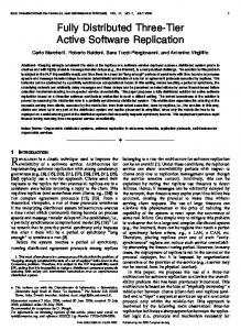
for details). It might also come as a surprise that both the exact identity of a node (j) and the parameter of TSLS(k) are not present. The parameter k is implicitly mapped to q because q becomes relevant as an approximation only when there are many rounds in the improvement step of TSLS(k). When there is only one round (as in TSLS) or just a few (when k is large), then the method by which q is derived becomes less accurate. For sufficiently small k (that lead to many rounds), the exact value of k does not affect q.3 Similarly, the lack of j in Eq. (3) means that q captures the amount of improvement that is available to all nodes, irrespectively of the exact identity (turn) of each one. As will be shown shortly, this is the basic amount of improvement to consider under TSLS(k), whereas the exact identity has a negligible additional contribution. Due to the rather elaborate form of Eq. (3) it is difficult to understand the behavior of q by inspection only; it is very easy, however, to use (3) for producing graphs that reveal its behavior. For this purpose, we consider a group in which the access costs are tl = 0, tr = 1, ts = 2 and we plot q for two kinds of power-law demands, a = 0.4 and a = 0.8 (Fig. 2) and for varying n, C. The two figures show that there are significant performance gains under TSLS(k). The gain of each and every node of the group can double with respect to the corresponding GL one under a = 0.4 whereas it can be significant (25% improvement) under the more skewed demand a = 0.8. The improvement increases with larger groups (n) as more 3
The value of k affects GEQ j , and thus qj also, marginally through the gain component (iii) (defined in Appendix B). As this
gain component is typically very small, it is ignored in the derivation of Eq. (3).
16
C
C
100 80
60 40
40
20
20
2.2
1.25
2
q
100 80
60
q
1.2
1.8
1.15
1.6
1.1 20
20 40
40 60
n Figure 2:
60
n
80 100
80 100
Illustration of the behavior of q under power-law demand for two values of the skewness parameter: a = 0.4 (left
graph) and a = 0.8 (right graph). The access costs are: tl = 0, tr = 1, ts = 2.
objects become available from remote nodes. It decreases as the nodes become larger (C), in which case the GL placement includes most of the valuable objects. In Tables 3, 4 we compare the q obtained from the previous examples with min qj and avg qj obtained by executing TSLS(k) for k = 1. The main conclusion from these tables is that the approximate analytic expression q is very close (typically within 1-2%) to the actual min qj and avg qj from the execution of TSLS(k). The fact that min qj and avg qj and the approximation (that does not consider specific nodes) are so close to each other, points to the fact that for sufficiently small k, the identity of a node has a negligible effect on its gain under TSLS(k).
7
A protocol for applying the Nash equilibrium for DSR
In this section we outline a protocol for implementing TSLS or TSLS(k) in a distributed replication group.
7.1
Deciding turns for the improvement step
First, we describe a simple way for deciding turns that can be used with both TSLS and TSLS(k); for TSLS the ordering has an impact on the individual gains, whereas for TSLS(k) under small k, the ordering has a diminishing effect on the gains. Consider an arbitrary labelling of nodes, not related to the ordering in which nodes take turns. Let Th denote a “merit” quantity associated with node vh , 1 ≤ h ≤ n, based on which vh ’s turn is decided. Th 17
C
5
n
10
15
20
C
50
75
100
q
1.404
1.392
1.385
min qj
1.438
1.432
1.430
avg qj
1.440
1.422
q
1.620
min qj
1.632
50
75
100
q
1.096
1.089
1.085
min qj
1.101
1.096
1.093
1.431
avg qj
1.102
1.096
1.093
1.602
1.592
q
1.131
1.121
1.116
1.625
1.621
min qj
1.125
1.119
1.116
5
n
10
avg qj
1.634
1.626
1.622
avg qj
1.125
1.119
1.116
q
1.725
1.704
1.692
q
1.145
1.135
1.129
min qj
1.726
1.718
1.711
min qj
1.135
1.130
1.125
avg qj
1.728
1.719
1.712
avg qj
1.136
1.130
1.126
q
1.787
1.764
1.752
q
1.152
1.142
1.136
min qj
1.776
1.764
1.761
min qj
1.140
1.135
1.130
avg qj
1.778
1.765
1.761
avg qj
1.141
1.135
1.130
Table 3:
15
20
Table 4:
Comparison of the approximate analytic expres-
Comparison of the approximate analytic expres-
sion q to the actual qj ’s from executing TSLS(k) under power-
sion q to the actual qj ’s from executing TSLS(k) under power-
law demand a = 0.4 and tl = 0, tr = 1, ts = 2.
law demand a = 0.8 and tl = 0, tr = 1, ts = 2.
will be defined in such a way that larger ids will be assigned to nodes having larger values of Th . At the end, a node whose value of Th is the jth largest one, will be re-labelled vj , thus taking the jth turn. There are many ways to define Th for a node; among them the following three are of particular interest because they can be naturally associated with a common case in which nodes have similar demand patterns and where a higher turn is better (see Sect. 5.2): ⎧ ⎪ ⎪ (proportional fairness) C ⎪ ⎨ h Th = (pro social benefit) ρh ⎪ ⎪ ⎪ ⎩ C ·ρ (hybrid) h
h
The first one caters to proportional fairness. It suggests that a node’s turn, or equivalently its share of the extra gain produced through the cooperation, be proportional to the amount of resource (storage capacity) that the node contributes. Under such Th , vj is the jth largest node. The second definition is a socially inclining one. It favors nodes that generate more requests, as these nodes have the largest influence on the social utility. Under such Th , vj is the jth more active node. Notice that following such a criterion for deciding turns is by no means equivalent to the Socially Optimal (SO) strategy. An equilibrium placement under the pro social benefit criterion favors active nodes by allocating them a bigger share of the extra 18
gain produced through the cooperation; this is to say that all other nodes will have (at least) their GL gain intact, whereas under SO, the benefited nodes may cause other nodes to fall below the GL level of gain. The third expression for Th is a hybrid way of splitting the gains of the cooperation; it favors nodes that contribute more storage and also produce more requests. Having defined the criterion based on which turns are decided, we move on to defining a protocol for implementing the algorithms and obtaining the equilibrium placement that corresponds to the decided ordering.
7.2
Distributed protocol
A straightforward centralized implementation would require each node to report rj and Cj to a central node responsible for executing the TSLS algorithm and sending back the placements Pj . The problem with such a centralized architecture is that it requires transmitting n rate vectors rj , with each one containing N (object id, request probability) pairs; for large N this can lead to the consumption of too much bandwidth by all nodes as much as by the central node, which has to send back the placements. We, therefore, turn our attention to the development of the following fully distributed protocol which involves three phases: Phase DT: During this phase, turns are decided. 1. Each node vh multicasts4 to the group its merit pair (Ch , ρh ), while listening for, and storing, such pairs from other nodes. The truthfulness of the transmitted pair is crosschecked later on by other nodes during the operation of the distributed group. 2. Having listened to n − 1 other merit pairs, each node may compute its turn j based on a pre-agreed definition of Th . Phase 0: In this phase the initial placements according to TSLS are computed and distributed. 1. Each node vj computes its initial placement Pj0 and multicasts it to the group. Taking turns is not required at this phase and nodes may transmit their information concurrently. 4
Native, or end-system, multicast can be employed.
19
2. Nodes listen and store the initial placements of other nodes. Phase 1: In this phase, the initial placements of TSLS are improved. 1. Node vj waits for its turn (i.e., until vj−1 completes its own turn and transmits) and then computes its improved placement Pj1 as described by TSLS. 2. Following the computation of Pj1 , node vj transmits Ej1 and Ij1 to the group. 3. Nodes vj � , j < j � ≤ n receive Ej1 and Ij1 and use them to produce Pj1 using also Pj0 , which they have from Phase 0. To implement the TSLS(k) algorithm, Phase 1 needs to be repeated until no node has any more changes to perform. As was mentioned earlier, TSLS(k) provides a tradeoff between the improved fairness and the increased time required to perform multiple rounds at Phase 1. The volume of transmitted information, however, is essentially the same as with the baseline TSLS. The aforementioned protocol has several advantages. It achieves a degree of parallelism, by permitting nodes to compute their initial placements during Phase 0 independently and concurrently with other nodes. Phase 1 involves a distributed computation too, albeit a sequential one. The major advantage, however, relates to the reduction in the amount of transmitted information as compared to a centralized computation which requires the transmission of n·N � pairs (object id, request frequency) towards the central point and then vj ∈V Cj object ids sent back from the central point to the nodes carrying the placements Pj1 . Our protocol limits � the amount of transmitted information to less than 3 · vj ∈V Cj object ids (initial placements plus eviction and insertion sets, with the worst case occurring when all nodes change all their objects at the improvement step ). This represents a substantial reduction in the amount of transmitted information, as typically the number of available objects is several orders of magnitude larger than the aggregate storage capacity of the group. Furthermore, lists of object ids can be represented succinctly by employing simplr compression techniques such as Bloom filters [19, 3], whereas rate vectors composed of (object id, request frequency) elements, are much harder to represent and communicate. In the above protocol, the transmitted information could be reduced further by not sending Ej1 ’s. The TSLS algorithms needs to know whether at least one copy of an object exists 20
somewhere in the group, and not its exact location. Proposition 2 guarantees that evicted objects are multiple ones, so specifying the eviction set of each node is not required for the execution of TSLS as it is guaranteed that evicted objects exist elsewhere in the group. Transmitting the Ej1 ’s, however, is valuable for the purpose of truthfulness checking. Having Pj0 , Ij1 and Ej1 , every node can compute the final placement Pj1 of every other node vj . Then, if a node requests an object oi that appears to belong to Pj1 , but vj fails to deliver it, then this can be taken as an indication that vj has been untruthful. A node may be tempted to be untruthful and, say, declare at Phase DT a storage capacity that is larger than its actual one. The purpose for doing that is that under TSLS and the proportional fairness criterion, such a false declaration can lead to the assignment of a higher, thus better, turn (on the other, if TSLS(k) is employed, ordering is of limited importance). Knowing the exact placement of other nodes guards against such exploitations as untruthful nodes can be disclosed. Similar checks can be performed regarding the declared request rate.
8
Numerical examples
In this section we present some simple numerical examples mostly for the purpose of demonstrating the operation of TSLS and TSLS(k). When comparing against the social optimal placement, we use the method of Leff et al. [1] (Appendix C) to obtain it. In the first example, there are two nodes that generate requests following the exact same Zipf-like distribution, i.e., rij = ρj · K/ia . The local access cost is, tl = 0, the remote one, tr = 1, and the cost of accessing the origin server, ts = 2; this leads to a hop-count notion of distance. There are N = 100 distinct objects, and each node has a capacity for C = 40 objects. In Table 5 we show the objects replicated under the GL, SO, and EQ replications strategies for fixed ρ1 = 1 and varying ρ2 ; here the EQ strategy is produced by the baseline TSLS. The GL strategy selects for each node the first 40 most popular objects, i.e., those with ids in {1:40}, independently of ρ2 . The SO strategy, however, is much different. As the request rate from Node 2 increases, SO uses some of the storage capacity of Node 1 for replicating objects that do not fit in Node 2’s cache, thereby depriving Node 1 of valuable storage capacity for its own objects. For ρ2 = 10, Node 1 gets to store only 3 of its most popular objects, while
21
placement strategy
Node 1 objects
Node 2 objects
GL, ρ2 = X
{1:40}
{1:40}
SO, ρ2 = 1
{1 : 16} ∪ {41 : 64}
{1:40}
SO, ρ2 = 2
{1 : 12} ∪ {41 : 68}
{1:40}
1.6 1.55
1.7
v2 – SO 1.65
{1 : 9} ∪ {41 : 71}
{1:40}
{1 : 7} ∪ {41 : 73}
{1:40}
SO, ρ2 = 5
{1 : 6} ∪ {41 : 74}
{1:40}
SO, ρ2 = 6
{1 : 5} ∪ {41 : 75}
{1:40}
1.45
SO, ρ2 = 7
{1 : 4} ∪ {41 : 76}
{1:40}
1.4
SO, ρ2 = 8
{1 : 4} ∪ {41 : 76}
{1:40}
SO, ρ2 = 9
{1 : 3} ∪ {41 : 77}
{1:40}
SO, ρ2 = 10
{1 : 3} ∪ {41 : 77}
{1:40}
EQ, ρ2 = X
{1 : 23} ∪ {41 : 57}
{1:40}
Table 5:
gain Gj
SO, ρ2 = 3 SO, ρ2 = 4
1.5
v2 – EQ (TSLS)
v2 – EQ (TSLS(1))
v1 – EQ (TSLS)
v1 – EQ (TSLS(1))
v1, v2 – GL v1 – SO
1.35 1.3 1
2
3
4
5
6
7
8
9
ρ2 (request rate of v2)
Figure 3:
An example with v1 , v2 having the same Zipf-
Individual node gains for the example of Ta-
like demand pattern with a = 0.8. The number of available
ble 5. “vj – XX” denotes the gain for node vj under the
objects is N = 100 and the storage capacity of each node is
placement strategy XX.
C = 40. Also, tl = 0, tr = 1, ts = 2, ρ1 = 1.
it uses the rest of its storage for picking up the next 37 more popular objects for Node 2, starting with the one with id 41. Under the EQ strategy Node 1 (v1 ) stores 23 of its most popular objects. Node 2 (v2 ) is the second one (i.e., the last one) to improve its placement, and it naturally selects the initial 40 most popular objects. We now turn our attention to the gain Gj of the two nodes under the various placement strategies (the corresponding access cost can be obtained from the expression ts −Gj ). Figure 3 shows that as ρ2 increases, the gain of v2 under SO increases as it consumes storage from v1 for replicating objects according to its preference; v1 ’s gain under SO decreases rapidly as a result of not being able to replicate locally some of its most popular objects. In fact, for ρ2 > 2.5, v1 ’s gain becomes worse (lower) that the corresponding one under GL. From this point and onwards, v1 is being mistreated by the SO strategy and thus has no incentive in participating in it, as it can obviously do better on its own under a GL placement. By following an EQ strategy, a node’s gain is immune to the relative request intensities and this is why the EQ lines are parallel to the x-axis of Fig. 3. v1 ’s gain under the EQ produced by TSLS is immune to the increasing ρ2 and strictly higher than its gain under GL. This demonstrates the fact that the EQ strategy avoids the mistreatment problem. Under the EQ produced by TSLS both nodes achieve higher gains than with GL, but it is v2 that benefits the most, and thus incurs a higher gain than v1 . This owes to the fact that v2 is 22
10
Table 6:
algorithm
Node 1 objects
Node 2 objects
TSLS
{1 : 23} ∪ {41 : 57}
{1:40}
TSLS(1)
{1 : 23} ∪ {25, 27, 29, 31 . . . , 55, 57}
{1 : 23} ∪ {24, 26, 28, 30, . . . , 54, 56}
TSLS(2) .. .
{1 : 23} ∪ {25, 26, 29, 30 . . . , 53, 54, 57} .. .
{1 : 24} ∪ {27, 28, 31, 32 . . . , 55, 56} .. .
TSLS(17) .. .
{1 : 23} ∪ {41 : 57} .. .
{1:40} .. .
TSLS(40)
{1 : 23} ∪ {41 : 57}
{1:40}
An example of the placement produced by TSLS and TSLS(k). Here v1 , v2 have the same Zipf-like demand pattern
with a = 0.8. The number of available objects is N = 100 and the storage capacity of each node is C = 40. Also, tl = 0, tr = 1, ts = 2.
the second (last) one to improve its placement and, thus, has an advantage under TSLS as discussed in Sect. 5.2. The difference in performance between the two nodes can be eliminated by employing the TSLS(k) algorithm. To show this, Fig. 3 includes the gains of the two nodes under the EQ strategy that is produced by TSLS(1). The corresponding lines almost coincide, which demonstrates the ability of TSLS(k) to be fair and to assign identical gains to v1 and v2 (as opposed to TSLS which, in this example, favors v2 ). The placements produced by TSLS(k) (for the previous example) are exemplified in Table 6 for different values of k. The round-robin k-constrained operation of TSLS(k) is evident in the produced placements. For example TLSL(1) places in each one of the two nodes the first 23 most popular objects, while it assigns the next 34 objects (object 24 - object 57) to the two nodes interchangeably. TSLS(2) similarly, assigns the initial most popular objects to both nodes, while it assigns the rest most popular ones (up to the available storage capacity) interchangeably, two objects at a time. TSLS(k) operates similarly for larger k, up to k = 17, at which point it reduces to the baseline TSLS. In the previous example, the equilibrium strategy for v2 identified by the TSLS algorithm, P21 , was identical to its GL strategy P20 , i.e., v2 made no changes to its initial placement during the improvement step of TSLS (on the other hand, v1 changed its initial placement during the improvement step). This has been a consequence of the fact that both nodes followed the exact same demand pattern. This is not, however, the case in general. The following example, depicted in Table 7, demonstrates an example in which both nodes improve their initial placements. The left portion of the table shows the object popularity ranking which,
23
node object popularity ranking (decreasing order)
init. placement
impr. placement eviction set insertion set
v1
4 7 5 3 2 9 1 8 10 6
P10
= {4, 7, 5, 3}
P11 = {4, 7, 5, 1}
E11 = {3}
I11 = {1}
v2
2 9 3 5 6 1 4 8 7 10
P20 = {2, 9, 3, 5}
P21 = {2, 9, 3, 6}
E21 = {5}
I21 = {6}
Table 7:
An example with v1 , v2 having different demand patterns. Here the number of available objects is N = 10 and the
storage capacity of each node is C = 4. The demand pattern of each node is Zipf-like with a = 0.8 but the popularity ranking is different for the two nodes.
in this example, is not the same for both nodes; v1 ’s object ranking in decreasing order of popularity is 4, 7, 5, . . . , 6, while for v2 it is 2, 9, 3, . . . , 10. The right part of the table depicts the initial placement, the improved placement, as well as the insertion and eviction sets for the two nodes. Notice that v1 evicts object 3 which is included in the initial placement of v2 and inserts in its position the next most valuable object that is not included in the initial placement of v2 , which is object 1. Then v2 takes turn in improving its initial placement and evicts object 5 to insert object 6. The resulting placement (P11 , P21 ) is an equilibrium pair.
9
Related work
We are aware of only a few very recent works on game-theoretic aspects of object replication. The most relevant to our work is the one due to Chun et al. [28], which studies distributed selfish replication (despite calling it caching). However, this work does not consider storage capacity limits on the nodes, while it also addresses more complex payment games and, thus, differs substantially from our approach. Another related work is due to Er¸cetin and Tassiulas [29], on market-based resource allocation in content delivery networks. Their focus, however, is on a three-part market game between content providers, distributors, and consumers, and thus they consider only very simple object replication strategies (greedy local ones). Our work on distributed selfish caching in [17] is, to the best of our knowledge, the only one studying similar problems under distributed caching (looking at different replacement algorithms, cache configurations and inter-cache cooperation schemes). Recent works on incentives in P2P networks, e.g., Antoniadis et al. [30], study the problem of attracting users to a P2P network and making them contribute more content. The aforementioned work and other similar ones, formulate the problem at a completely different level as compared to our work, as they focus on the number of files shared by each node, without identifying the 24
identities of these files, whereas we focus on identifying the exact set of files shared.
10
Conclusions and future work
This work has described two algorithms and an efficient distributed protocol for implementing equilibrium object placement strategies in a distributed selfish replication group. Such placement strategies become meaningful when replication nodes cater to their local utilities, as is the case with some content distribution applications that are run under multiple authorities (e.g., P2P, distributed web caching). In such applications, following a socially optimal placement strategy may lead to the mistreatment of some nodes, possibly causing their departure from the group. Our equilibrium strategies on the other hand, guarantee that all nodes are better off participating in the group as opposed to operating in isolation in a greedy local manner. This keeps a distributed group from splitting apart, by creating an excess gain for all (stemming from the cooperation) while forbidding the mistreatment of any one of the nodes. An interesting line for future work is to investigate the case that nodes are allowed to communicate and negotiate to form alliances. Such alliances would cooperate and try to secure for each one of their members a gain that is potentially higher than the one that each member can achieve by acting selfishly on its own. This would require, however, additional protocols and mechanisms to be installed, thus increasing the overall complexity (computational and exchange of information) as compared to the complexity which is required for implementing the presented equilibrium strategies.
References [1] Avraham Leff, Joel L. Wolf, and Philip S. Yu, “Replication algorithms in a remote caching architecture,” IEEE Transactions on Parallel and Distributed Systems, vol. 4, no. 11, pp. 1185–1204, Nov. 1993. [2] Duane Wessels and K. Claffy, “ICP and the Squid web cache,” IEEE Journal on Selected Areas in Communications, vol. 16, no. 3, Apr. 1998.
25
[3] Li Fan, Pei Cao, Jussara Almeida, and Andrei Z. Broder, “Summary cache: a scalable wide-area web cache sharing protocol,” IEEE/ACM Transactions on Networking, vol. 8, no. 3, pp. 281–293, 2000. [4] Jianping Pan, Y. Thomas Hou, and Bo Li, “An overview DNS-based server selection in content distribution networks,” Computer Networks, vol. 43, no. 6, Dec. 2003. [5] I. Stoica, R. Morris, D. Liben-Nowell, D.R. Karger, M.F. Kaashoek, F. Dabek, and H. Balakrishnan, “Chord: A scalable peer-to-peer lookup protocol for internet applications,” IEEE/ACM Transactions on Networking, vol. 11, no. 1, pp. 17–32, 2003. [6] P. Krishnan, Danny Raz, and Yuval Shavit, “The cache location problem,” IEEE/ACM Transactions on Networking, vol. 8, no. 5, pp. 568–581, Oct. 2000. [7] Bo Li, Mordecai J. Golin, Giuseppe F. Italiano, Xin Deng, and Kazem Sohraby, “On the optimal placement of web proxies in the internet,” in Proceedings of the Conference on Computer Communications (IEEE Infocom), New York, Mar. 1999. [8] Lili Qiu, Venkata Padmanabhan, and Geoffrey Voelker, “On the placement of web server replicas,” in Proceedings of the Conference on Computer Communications (IEEE Infocom), Anchorage, Alaska, Apr. 2001. [9] Eric Cronin, Sugih Jamin, Cheng Jin, Anthony R. Kurc, Danny Raz, and Yuval Shavitt, “Constraint mirror placement on the internet,” IEEE Journal on Selected Areas in Communications, vol. 20, no. 7, Sept. 2002. [10] Madhukar R. Korupolu, C. Greg Plaxton, and Rajmohan Rajaraman, “Placement algorithms for hierarchical cooperative caching,” in Proceedings of the 10th Annual Symposium on Discrete Algorithms (ACM-SIAM SODA), 1999, pp. 586 – 595. [11] Konstantinos Kalpakis, Koustuv Dasgupta, and Ouri Wolfson, “Optimal placement of replicas in trees with read, write, and storage costs,” IEEE Transactions on Parallel and Distributed Systems, vol. 12, no. 6, pp. 628–637, June 2001.
26
[12] Jussi Kangasharju, James Roberts, and Keith W. Ross, “Object replication strategies in content distribution networks,” Computer Communications, vol. 25, no. 4, pp. 376–383, Mar. 2002. [13] Ivan D. Baev and Rajmohan Rajaraman, “Approximation algorithms for data placement in arbitrary networks,” in Proceedings of the 12th Annual Symposium on Discrete Algorithms (ACM-SIAM SODA), Jan. 2001, pp. 661–670. [14] Thanasis Loukopoulos and Ishfaq Ahmad, “Static and adaptive distributed data replication using genetic algorithms,” Journal of Parallel and Distributed Computing, vol. 64, no. 11, pp. 1270–1285, Nov. 2004. [15] Nikolaos Laoutaris, Vassilios Zissimopoulos, and Ioannis Stavrakakis, “Joint object placement and node dimensioning for internet content distribution,” Information Processing Letters, vol. 89, no. 6, pp. 273–279, Mar. 2004. [16] Nikolaos Laoutaris, Vassilios Zissimopoulos, and Ioannis Stavrakakis, “On the optimization of storage capacity allocation for content distribution,” Computer Networks, vol. 47, no. 3, pp. 409–428, Feb. 2005. [17] Nikolaos Laoutaris, Georgios Smaragdakis, Azer Bestavros, and Ioannis Stavrakakis, “Mistreatment in distributed caching groups: Causes and implications,” Technical Report BUCS-TR-2005-026, Compter Science Department, Boston University, Boston, MA, July 2005. [18] Martin J. Osborne and Ariel Rubinstein, A Course in Game Theory, MIT Press, 1994. [19] Burton Bloom, “Space/time trade-offs in hash coding with allowable errors,” Communications of the ACM, vol. 13, no. 7, pp. 422–426, July 1970. [20] John W. Byers, Jeffrey Considine, Michael Mitzenmacher, and Stanislav Rost, “Informed content delivery across adaptive overlay networks,” IEEE/ACM Transactions on Networking, vol. 12, no. 5, pp. 767–780, Oct. 2004. [21] Andrei Broder and Michael Mitzenmacher, “Network applications of Bloom filters: A survey,” Internet Mathematics, 2004, [accepted for publication]. 27
[22] D. Karger, E. Lehman, F.T. Leighton, M. Levine, D. Lewin, and R. Panigrahy, “Consistent hashing and random trees: Distributed caching protocols for relieving hot spots on the World Wide Web,” in Proceedings of the 29th Annual Symposium on Theory of Computing (ACM STOC), May 1996, pp. 654–663. [23] A. Leff, L. Wolf, and P. S. Yu, “Efficient LRU-based buffering in a LAN remote caching architecture,” IEEE Transactions on Parallel and Distributed Systems, vol. 7, no. 2, pp. 1991–205, Feb. 1996. [24] Christos H. Papadimitriou and Kenneth Steiglitz, Combinatorial Optimization: Algorithms and Complexity, Dover Publications, New York, 1998. [25] Nikolaos Laoutaris, Orestis Telelis, Vassilios Zissimopoulos, and Ioannis Stavrakakis, “Distributed selfish replication,”
Technical Report, Department of Informat-
ics and Telecommunications, University of Athens, 2005,
available on-line at:
http://www.cnl.di.uoa.gr/∼laoutaris/cgame TECH.pdf. [26] Lee Breslau, Pei Cao, Li Fan, Graham Philips, and Scott Shenker, “Web caching and Zipf-like distributions: Evidence and implications,” in Proceedings of the Conference on Computer Communications (IEEE Infocom), New York, Mar. 1999. [27] Anirban Mahanti, Carey Williamson, and Derek Eager, “Traffic analysis of a web proxy caching hierarchy,” IEEE Network, vol. 14, no. 3, pp. 16–23, May 2000. [28] Byung-Gon Chun, Kamalika Chaudhuri, Hoeteck Wee, Marco Barreno, Christos H. Papadimitriou, and John Kubiatowicz, “Selfish caching in distributed systems: A gametheoretic analysis,” in Proc. ACM Symposium on Principles of Distributed Computing (ACM PODC), Newfoundland, Canada, July 2004. ¨ ur Er¸cetin and Leandros Tassiulas, “Market-based resource allocation for content [29] Ozg¨ delivery in the internet,” IEEE Transactions on Computers, vol. 52, no. 12, pp. 1573– 1585, Dec. 2003.
28
[30] Panayotis Antoniadis, Costas Courcoubetis, and Robin Mason, “Comparing economic insentives in peer-to-peer networks,” Computer Networks, vol. 46, no. 1, pp. 1–146, Sept. 2004. [31] Xueyan Tang and Samuel T. Chanson, “Adaptive hash routing for a cluster of clientside web proxies,” Journal of Parallel and Distributed Computing, vol. 64, no. 10, pp. 1168–1184, Oct. 2004. [32] R.S. Garfinkel and G.L. Nemhauser, Integer Programming, Wiley, New York, 1972.
A A.1
Proofs of Propositions 1-6 Proposition 1
Re-write Gj (P ) from Eq. (1) as follows: ⎛
⎞
� � ⎜ � ⎟ ⎟ Gj (P ) = ⎜ r · (t − t ) + r · (t − t ) + rij · (ts − tr ) ij s l ij r l ⎠ ⎝ oi ∈Pj oi ∈P / −j
oi ∈Pj oi ∈P−j
(4)
oi ∈P−j
The new expression is derived by considering objects that are replicated at vj and again elsewhere in the group, and re-expressing their gain by splitting it into two parts through rij · (ts − tl ) = rij · (ts − tr ) + rij · (tr − tl ). Notice now that given P−j , the quantity outside the parenthesis of Eq. (4) becomes a constant, i.e., it does not depend on the objects selected for replication at vj . Thus to maximize Gj (P ) amounts to maximizing the quantity inside the parenthesis. The quantity inside the parenthesis depends on both the objects replicated at other nodes, and the objects selected for replication at vj ; it is the exact quantity that is maximized by solving the aforementioned 0/1 Knapsack problem (notice that Eq. (4) is composed of the gijk values of objects that are considered in the 0/1 Knapsack formulation). This proves the claim of the proposition.
29
A.2
Proposition 2
Consider two objects oie ∈ Ej1 and oii ∈ Ij1 . By their definition oie ∈ Pj0 and oii ∈ / Pj0 which implies that: gi0e j ≥ gi0i j
(5) −
1 Suppose now that contrary to the claim of the proposition oie ∈ / (Pj0 ∩ P−j ) which translates −
1 / P−j since oie ∈ Pj0 . Since oii is inserted in place of the evicted oie at the improvement to oie ∈
step, it must be that: gi1i j > gi1e j
(6)
−
1 / P−j , oie retains its Step 0 gain (by definition of gijk ), hence: Since oie ∈
gi1e j = gi0e j
(7)
Finally, from the definition of the gain function in Eq. (2): gi1i j ≤ gi0i j
(8)
gi1i j > gi0e j
(9)
Combining equations (6), (7) gives:
Multiplying Eq. (8) by −1 and adding side-by-side with Eq. (9) leads to gi0e j < gi0i j which is −
1 clearly false as it contradicts Eq. (5). Thus it must be that oie ∈ (Pj0 ∩ P−j ), which proves
the claim of the proposition.
A.3
Proposition 3
Before going into the proof, notice that since all accesses to objects at remote nodes cost the same, the following observation can be written with regard to the ratio between the gain of a represented object and the gain of the same object when it is unrepresented. −
1 Observation 1 For all oi ∈ P−j and all vj ∈ V ,
1 gij 0 gij
=
rij (tr −tl ) rij (ts −tl )
=
tr −tl ts −tl
= τ < 1.
In other words, the relative reduction of gain between represented and unrepresented objects is the same for all different objects and all different nodes.
30
Consider now two object oie ∈ Ej1 and oii ∈ Ij1 . By their definition oie ∈ Pj0 and oii ∈ / Pj0 which implies that: gi0e j ≥ gi0i j
(10)
Since oii is inserted in place of the evicted oie at the improvement step, it must be that: gi1i j > gi1e j
(11)
−
1 Proposition 2 gives that oie ∈ P−j ; combined with Observation 1 this leads to:
gi1e j = τ · gi0e j
(12) −
1 Suppose now that contrary to the claim of the proposition, oii ∈ (Pj0 ∪ P−j ) which translates −
1 to oii ∈ P−j since oii ∈ / Pj0 . By using Observation 1, this assumption leads to:
gi1i j = τ · gi0i j
(13)
Substituting (12), (13) in (11) we can write τ · gi0i j > τ · gi0e j , which simplifies to: gi0i j > gi0e j
(14) −
1 Inequality (14) is clearly false as it contradicts with (10). Thus it must be that oii ∈ / (Pj0 ∪P−j ),
which proves the claim of the proposition.
A.4
Proposition 4
1 1 1 Let P−j = P11 ∪ . . . ∪ Pj−1 ∪ Pj+1 ∪ . . . ∪ Pn1 denote the set of objects collectively held by nodes −
1 1 other than vj at the end of TSLS; notice that generally P−j �= P−j (the latter refers to the
set of objects collectively held by the other nodes during vj ’s turn at the improvement step). To prove the proposition, it suffices to show that for every node vj ∈ V , Gj (P 1 ) ≥ 1 1 Gj ((P11 , . . . , Pj−1 , Pj , Pj+1 , . . . , Pn1 )), for all Pj ∈ {Pj } (recall that {Pj } denotes the set of
placement strategies for node vj ). As Proposition 1 states that solving the 0/1 Knapsack −
1 problem under given P−j maximizes vj ’s gain, what we need to show here is that solving the −
1 1 instead of P−j , leads again to the same placement Pj1 , i.e., 0/1 Knapsack, this time under P−j −
1 1 ) = Greedyj (P−j ), and that this holds true for all vj , 1 ≤ j ≤ n − 1 (it obviously Greedyj (P−j
holds true for j = n). In other words, we need to show that for all vj , the changes in the 31
global placement contributed by the nodes that improved their placements following vj ’s turn, do not affect the optimality of vj ’s placement, as it was determined at the time of its turn. Looking at a given vj , the differences between the global placements at vj ’s turn and at the termination of TSLS are determined by: (a) the multiples that were evicted, i.e., Eh1 ’s, and (b) the unrepresented ones that were inserted, i.e., Ih1 ’s, j + 1 ≤ h ≤ n. We will show that −
1 1 these changes do not affect the optimality of Pj1 , i.e., Pj1 = Greedyj (P−j ) = Greedyj (P−j ). −
1 , but was later evicted by some of the node(s) Consider oie , an object that belonged to P−j
that were holding it during vj ’s turn. Proposition 2 guarantees that in the end at least one node will still be replicating oie , i.e., oie ∈ P 1 . This precludes the case that vj would decide / Pj1 . If on the other hand, oie ∈ Pj1 to modify Pj1 so as to include oie , in the case that oie ∈ then again the evictions of some multiple copies of oie at remote nodes cannot trigger changes to Pj1 . Consider now oii , an object that was inserted by a node following vj ’s turn. Proposition 3 guarantees that oii is an unrepresented one, which in turn means that oii ∈ / Pj1 . This in effect means that its insertion may not cause the reduction of the gijk value of any object oi ∈ Pj1 , as the only such object that would be affected (its value be reduced thus making it eligible for eviction), would be oi = oii ; oii however does not belong to Pj1 . The previous two arguments regarding oie and oii guarantee that node vj has no reason to change Pj1 as a result of the −
1 1 transition from P−j to P−j , and this holds true for all vj . Combining the previous with the 1 (stems from Proposition 1), establishes that P 1 is a pure fact that Pj1 maximizes Gj given P−j
Nash equilibrium for DSR.
A.5
Proposition 5
Since N and Cj ’s are all finite, in order for TSLS(k) not to terminate in a finite number of rounds, it would require it to enter a loop, in which some objects would be evicted and then be re-inserted indefinitely. Propositions 2 and 3, however, which also apply to TSLS(k), don’t permit for such loops to occur. This is because they establish: (1) that only multiple objects may be evicted, and (2) that only unrepresented objects may be inserted. Since the number of objects N is finite, this guarantees that the elimination of the unprofitable multiple objects will be completed after a finite number of rounds M . It also points to the fact that 32
M will be small, as each inserted object may be inserted by only one node (this precludes the visiting of all possible global placements, whose number is exponentially dependent on the input). To realize the stated upper bound on M , observe that it is the largest node that may perform the maximum number of changes, and thus cause the maximum number of rounds. For appropriately selected rate vectors rj , the largest node may change all its initial objects for new ones5 , and thus cause up to C max /k rounds.
A.6
Proposition 6
The Nash equilibrium property follows from the fact that at round M , all nodes are given the opportunity to improve their placements after observing the contents of other nodes, but no node has such an improvement to perform.
B
Derivation of q of Eq. (3)
A full round of the improvement step of TSLS(k) is defined to be a round in which each one of the n nodes performs the maximum number of allowed changes, that is k. Let R denote the last full round and let i be the index of the last object that is inserted by the last (the nth) node at the last full round. As each inserted object gets replicated only once in the group (Proposition 3) it is clear that i will be larger that any other index of an inserted object. Taking into consideration that objects 1 . . . C are represented in the group due to the initial GL placement, that the inserted objects are consecutive ones, and that nk unrepresented objects are inserted in total at each full round, we obtain that R =
i−C . nk
It is also possible to identify h, the index of the object whose place on the nth node is taken by i at the last full round. To do that we must take into consideration that with every batch of n − 1 consecutive full rounds: (i) nk of the least popular objects of the GL placement become “unique-ized”, i.e., are forced (through the evictions) to reside in only one node of the group (Proposition 2 guarantees that it is impossible to evict all the copies of an initially represented object); (ii) (n − 1)nk consecutive unrepresented objects are inserted; (iii) h reduces by nk as 5
This would require that all the objects in its initial placement be multiple ones, and that at least C max unrepresented objects
may profitably take their place. The second requirement can easily occur if the largest node requests objects with rates that tend to be uniformly distributed to the different objects.
33
compared to its value prior to the current batch of n − 1 full rounds.6 If R was a multiple of n − 1 then we would be able to accurately identify h through the following equation. h=C−
i−C (n + 1)C − i + n ·k+1= nk n
(15)
Given that the approximation that we are deriving is relevant when TSLS(k) performs many rounds, we can ignore the remainder of the integer division of R with n − 1 and retain (for the sake of simplicity) the h given by Eq. (15). Since we assumed that object i gets the position of object h, it must be that it leads to a higher excess gain for node n, i.e.: pi (ts − tl ) ≥ ph (tr − tl )
(16)
Substituting in Eq. (16) pi and ph (making use of our assumption that all nodes follow the same generalized power-law demand) and using also h from Eq. (15), we can write the following inequality for i: � i ≤ min
� (n + 1)C + n , nC , nφ + 1
where φ =
tr − tl ts − tl
a1 (17)
At this point we are ready to write an expression for GEQ j , the gain of the jth node under the into three components: (i) the gain EQ placement produced by TSLS(k). We will split GEQ j contributed by the initial (most popular) objects of the GL placement that are not affected by the improvement step (objects 1 . . . h − 1 which we denote by the set (H)); (ii) the gain contributed by any other object that does not belong to (H), but exists somewhere – locally or remotely – in the group (objects h . . . i fall in this category); (iii) the gain contributed by any object that does not belong to (H) but is replicated locally (in this category we have the set of objects (U) which comprises the unique-ized k-tuples that were kept locally, and the set of objects (I) which comprises the locally inserted objects). These sets are illustrated in Fig. 4. The objects of category (i) contribute to the overall gain with the product of their request probability times a weight (ts − tl ). The objects of category (ii) contribute similarly, but 6
To understand the eviction/insertion process see that at the first full round nodes 1 ≤ j ≤ n − 1 evict the same objects
C − k + 1 . . . C and insert different consecutive ones C + (j − 1)k + 1 . . . C + jk, while node n evicts a different set of objects C − 2k + 1 . . . C − k and inserts objects C + (n − 1)k + 1 . . . C + nk. The “unique-ized” objects of the first round (C − k + 1 . . . C) remain at node n. The unique-ized objects of the next full round (C − 2k + 1 . . . C − k) will remain at node n − 1, and so on until the completion of the (n − 1)th full round. Then another n − 1 batch of full rounds will begin, with node n being the one to sustain the currently unique-ized k-tuple of objects.
34
inserted objects (I) ( each square contains (n−1) slices with k consecutive objects in each slice ) obj 1
obj h−1
11 00 01 1 0 00 11 01 1 0 (H) initial GL part unique−ized GL objects (each slice a consecutive k−tuple)
Figure 4:
(U)
Tomography of the objects that are replicated at a node after the end of TSLS(k). (H) denotes the set of objects
that belong to the “head” of the GL placement, i.e., objects that are left intact by the improvement step because they are too valuable. (U) denotes the set of unique-ized objects, that is objects that were on the GL placement of all the nodes but were subsequently eliminated from all the nodes but the local one. (I) denotes the set of objects that were inserted locally by the improvement step.
with a smaller weight (ts − tr ) (the weight that amounts to a remote object). The objects by a partial weight of category (iii) are local objects; they have already contributed to GEQ j (ts − tr ) as they also belong to (ii), but must contribute by an additional weight (tr − tl ), so as to fill up to the weight (ts − tl ) that amounts to local objects (we have split the contribution of such objects in two parts similarly to what we have done in the proof of Proposition 1). The following approximate expression for GEQ considers only the contribution of (i) and (ii) j and disregards the contribution of (iii) which is typically very small (see Sect. 6.2): h−1 i � � 1 1 + (t − t )K s r a l la l=1 l=h � � (a) (a) (a) = (ts − tl )KHh−1 + (ts − tr )K Hi − Hh−1
GEQ ≈ (ts − tl )K j
(a)
In the previous expression, Hm =
�m l=1
(18)
1/la denotes the mth Harmonic number of order a.
(a)
When 0 ≤ a < 1, Hm can be approximated by its integral expression (see also [31]): � m m1−a − 1 (a) 1/la dl = Hm ≈ 1−a 1
(19)
The expression of vj ’s gain under the GL placement is much simpler: GGL = GGL = (ts − tl )KHC j
(a)
(20)
from Eq. (18) The approximation q of qj that is given in Eq. (3) is obtained by dividing GEQ j from Eq. (20), employing the integral approximation of Eq. (19), normalizing tr , ts with GGL j by considering tl = 0, and substituting h, i from Eqs (15), (17). 35
C
Socially optimal replication
Leff, Wolf and Yu [1] have derived the socially optimal replication strategy under a global utility by transforming the replica placement problem into a capacitated transportation problem [32] that can be solved efficiently in polynomial time. Let X = {Xij : 1 ≤ i ≤ N , 1 ≤ j ≤ n} be a matrix of binary decision variables Xij that equal 1 if object oi is replicated at node vj , and 0 otherwise; X defines a global placement. Also define zij , 1 ≤ i ≤ N , 1 ≤ j ≤ n + 1, as follows:
⎧ ⎨ r · (t − t ) ij r l zij = � ⎩ n� r � · (t − t ) r s j =1 ij
for 1 ≤ j ≤ n for j = n + 1
Leff, Wolf and Yu showed that the socially optimal replication strategy is given by the solution of the following capacitated transportation problem. maximize subject to
� �N f (X) = n+1 j=1 i=1 zij · Xij �n+1 1≤i≤N j=1 Xij ≥ 1, �N 1≤j≤n i=1 Xij ≤ Cj , �N j =n+1 i=1 Xij < ∞,
36