Oct 10, 2014 - Distributed SPS Algorithms for Non-Asymptotic. Confidence Region Evaluation. Francesca Bassi, Michel Kieffer, Vincenzo Zambianchi, Davide ...
Distributed SPS Algorithms for Non-Asymptotic Confidence Region Evaluation Francesca Bassi, Michel Kieffer, Vincenzo Zambianchi, Davide Dardari, Gianni Pasolini
To cite this version: Francesca Bassi, Michel Kieffer, Vincenzo Zambianchi, Davide Dardari, Gianni Pasolini. Distributed SPS Algorithms for Non-Asymptotic Confidence Region Evaluation. EuCNC 2014, Jun 2014, Bologne, Italy. pp.1-5, 2014, .
HAL Id: hal-01073681 https://hal-supelec.archives-ouvertes.fr/hal-01073681 Submitted on 10 Oct 2014
HAL is a multi-disciplinary open access archive for the deposit and dissemination of scientific research documents, whether they are published or not. The documents may come from teaching and research institutions in France or abroad, or from public or private research centers.
L’archive ouverte pluridisciplinaire HAL, est destin´ee au d´epˆot et `a la diffusion de documents scientifiques de niveau recherche, publi´es ou non, ´emanant des ´etablissements d’enseignement et de recherche fran¸cais ou ´etrangers, des laboratoires publics ou priv´es.
Distributed SPS Algorithms for Non-Asymptotic Confidence Region Evaluation Vincenzo Zambianchi, Michel Kieffer, Francesca Bassi, Gianni Pasolini, and Davide Dardari
Abstract—In this paper, the distributed computation of confidence regions for parameter estimation is considered. Some information diffusion strategies are proposed and compared in terms of the required number of data exchanges to get the corresponding region. The effects of algorithms truncation is also addressed. As support for the theoretical part, numerical results are presented.
I. I NTRODUCTION A wireless sensor network (WSN) is composed of powerconstrained sensing devices, cooperating in processing local measurements to complete a common task [1]. The task can be simple environmental monitoring (e.g., temperature, pollution levels) or the evaluation of a complex function of the measurements (e.g. localization of a source of signal [2]). The reference scenario considered here is the estimation of a parameter vector p∗ from the set of local and noisy measurements at the nodes. To provide coherent estimates at all nodes, robustness against equipment failure, and scalability versus network size, a distributed protocol working in absence of a central processing unit is desirable. In [3], [4] this is accomplished via recursive weighted least square estimation, where a consensus-based algorithm allows to incorporate information from neighbouring nodes in the local estimate. A similar approach is taken for the Bayesian framework in [5], where consensus-based distributed Kalman filtering is proposed. The algorithms in [3]–[5] converge asymptotically in time, but it is not possible to predict the quality of the local estimates in the non-asymptotic scenario without statistical knowledge of noise distribution. In some applications (e.g., in source localization) the characterization of the confidence region associated to the estimate can be more valuable than the evaluation of the point estimate itself. In this work we thus address the problem of the evaluation of non-asymptotic confidence regions for the estimation of p∗ . Non-asymptotic indicates that the estimate is evaluated from a finite amount of measurements (unlike classical Cramer-Rao bound-like asymptotic confidence regions). In the presence of a central processing unit the characterization of the non-asymptotic confidence regions can be accomplished using the results in [6]–[9]. Specifically, the methods in [6], [7] allow to derive a lower bound on the probability that p∗ falls within the confidence region, whereas Vincenzo Zambianchi, Davide Dardari and Gianni Pasolini are with CNIT, University of Bologna, Italy, Michel Kieffer is with L2S, CNRS, SUPELEC, Univ. Paris-Sud, Gif-sur-Yvette, France. Francesca Bassi is with ESMESudria, Ivry-sur-Seine, France. This work has been supported by the European commission within the NoE Newcom#.
the exact probability can be obtained using the sign perturbed sums (SPS) algorithm in [8]. In [9] efficient computation of the confidence regions is obtained using interval analysis techniques. These methods do not require precise statistical knowledge of the noise, and work under very mild assumptions on its distribution. The aim of this work is to provide fully distributed solutions for the in-node computation of the non asymptotic confidence regions, based on the SPS algorithm [8]. The SPS method is easily amenable to a distributed form, which converges in time to the centralized algorithm. We consider three distributed approaches (data flooding and parallel in-node processing, distributed processing via average consensus, and mixed flooding+consensus) able to provide exact confidence regions at each node, even for early truncation of the communication protocol. The performance is evaluated, for a target confidence level, in terms of the size of the confidence regions expressed as a function of the amount of data to be exchanged, and hence the energetic cost. This allows to compare the energetic efficiency of the proposed solutions. II. T HE C ENTRALIZED SPS A LGORITHM Let us recall, first of all, the centralized SPS algorithm [8] for the computation of non-asymptotic confidence regions. Consider a network of N nodes taking different noisy observations {yi }, for i = 1, 2, . . . , N , of a parameter p∗ belonging to the parameter space P, having dimension np . The following local linear scalar measurement model is considered for the ith node: yi = ψ Ti p∗ + wi ,
(1)
where ψ i is the regressor vector, supposed known only at the corresponding node i, and wi is the measurement noise. The only assumption we make on the measurement noise is that it is independent from node to node and its distribution is symmetric with respect to zero, this setting a quite general domain of applications. The SPS algorithm returns the exact confidence region ˆ of p∗�, obtained �as the around the least squares estimate p PN solution of the normal equations i=1 ψ i yi − ψ Ti p = 0. Specifically, define the unperturbed sum s0 (p) =
N X i=1
� � ψ i yi − ψ Ti p
(2)
and the m − 1 sign perturbed sums sj (p) =
N X
� � αj,i ψ i yi − ψ Ti p ,
(3)
i=1
where j = 1, . . . , m − 1 and αj,i ∈ {±1} are independent, identically distributed and equiprobable random signs, drawn at each node i. Given the squared norm of all previous quantities zj (p) = ||sj (p)||22 ,
j = 0, . . . , m − 1,
(4)
the confidence region Σq for the true parameter value p∗ is defined as Σq = {p ∈ P|z0 (p) is not among the q largest zj (p)} m−1 X τj (p) ≥ q , (5) = p ∈ P j=1 where τj (p) = 1 if zj (p) − z0 (p) > 0 and 0 otherwise. The rationale is that, for the true parameter value, the unperturbed sum is closely related to the measurement noise and it is therefore small, while for parameter values that are far from the true one, the perturbed sums are larger than the unperturbed one. In [8] it was proven that the confidence level is Prob(p∗ ∈ Σq ) = 1 −
q . m
(6)
It is worth noting that this algorithm requires a central entity with full knowledge of regressors ψ i , measurements yi , and coefficients αj,i . In the following section we will investigate three different solutions to overcome this limitation and let each node capable of computing (5) locally. III. I NFORMATION D IFFUSION S TRATEGIES This section presents three different solutions for the distributed evaluation of confidence regions. In all cases no central processing unit is assumed, hence confidence regions are locally evaluated at each node. The first solution here investigated is based on the flooding of all required quantities across the entire network and the subsequent in-node computation of the SPS algorithm. This will not only ensure that the computed confidence region is the same at all nodes, but also that it is exactly the same as in the centralized version of the algorithm. In the second solution, the information needed for the in-node computation of the SPS algorithm are, instead, exchanged according to an average consensus algorithm [10]. The third solution, whose details will be provided in the following, is a combination of flooding and consensus. Let us observe, finally, that for energy saving reasons, truncation of the information diffusion algorithms is often desirable. The effects of truncations in the considered algorithms is also investigated in subsection III-D. This constitutes, to the author knowledge, a relevant advance with respect to the current literature.
A. Information Diffusion Through Flooding In a flooding algorithm,h the generic node i initially broadi (0) casts its own state xi = ψ Ti , yi at time 0. At the successive step, it collects the states from neighbors, then forwards (1) a� new data packet containing� the aggregated state xi = � � n� �o n� �o ψ Ti , yi , ψ Tj , yj , where ψ Tj , yj dej∈Ni
j∈Ni
notes the set of regressors and measurements pairs collected from nodes j in the neighborhood Ni of node i. To avoid network collapse due to cycles, duplicated states are discarded. This process is repeated until each node in the network has collected the state from all nodes. Afterwards, each node is able to compute the perturbed and unperturbed sums in (2) and (3) for any p, and hence derive the confidence region. No transmission of αj,i is necessary, provided that all nodes agree on seeds for their random generators. Note that each node has (0) to transmit a packet containing Dflood = np + 1 values in (last) the first iteration and Dflood = N (np + 1) values in the last iteration. B. Information Diffusion Through Consensus Looking at (2) and (3) it is evident that the computation of s0 (p) and sj (p) does not necessarily require the knowledge of each single quantity, but rather of aggregated values. This suggests the adoption of consensus strategies that are well suited for distributed computation of sums or averages. A consensus scheme may be viewed as the following discrete time evolving system [10]–[12] x(k+1) = W x(k) (7) h iT (k) (k) (k) is the global state at where x(k) = x1 , x2 , . . . , xN time k, whose ith entry is the local state at node i. W is the system dynamic matrix that depends on the consensus algorithm as well as on network topology. Proper structures of W asymptotically lead to a global state whose entries are all equal to the average of the initial quantities x(0) [11], [12]. In particular, the convergence of the consensus algorithm is assured by the following three necessary and sufficient conditions: 1T W = 1T ,
W1 = 1,
ρ(W − 11T /N ) < 1
(8)
where ρ denotes the spectral radius (see [11]). We choose the Metropolis matrix, which allows a faster convergence than others. Each entry of the matrix is 1 if (i, j) ∈ E, 1+max{d Pi ,dj } 1− wi,q if i = j, (9) wi,j = (i,q)∈E 0 otherwise, where di = |Ni | denotes the degree of node i (i.e., the number of neighbors) and E is the set of edges in the network topology. According to (7), each node performs its local state update as follows N X (k+1) (k) wi,j xj . (10) xi = j=1
To the purpose of applying the described consensus algorithm to the problem of distributed calculation of (2) and (3), define the following averages that do not depend on p N 1 X ψ yi b0 = N i=1 i N 1 X A0 = ψ ψT N i=1 i i
N 1 X bj = αj,i ψ i yi N i=1
(11)
N 1 X Aj = αj,i ψ i ψ Ti N i=1
(12)
0.9 0.8 0.7 0.6
for j = 1, 2, . . . , m − 1. The consensus algorithm is launched on all Aj ’s and bj ’s (including b0 and A0 ). At step k = 0, the local state at node i is given by i x(0) = i h � � � T T T T (ψ i yi ) , ψ i ψ i , (αj,i ψ i yi ) j , αj,i ψ i ψ i j , with j = 1, 2, . . . , m − 1, that is, the single addends in (11) and (12). At each successive step the ith node updates its own state according to (10). Once a consensus on Aj and bj is reached, each node is able to locally evaluate (2) and (3) for any value p in the parameter search space. We want to underline that no particular value of the parameter p has to be transmitted and that getting averages, instead of the true sums, does not affect the SPS algorithm since the comparison of rescaled norms or norms gives the same ordering in (5). Therefore the algorithm works also without the knowledge of N . Note that the state is composed of Dcons = m(3np + n2p )/2 values, where symmetry of ψ i ψ Ti is exploited. The state dimension is constant during the entire running of the algorithm but is larger than that initially required by flooding. C. Mixed Flooding+Consensus Approach As observed, the pure average consensus algorithm requires an amount of data to be transmitted that is initially strictly larger than that required by flooding. However, in few iterations the amount of data transmitted with flooding exceeds Dcons due to data accumulation at nodes. This fact suggested the introduction of a third mixed strategy conceived as follows: flooding, as described in Sec. III-A, works until the amount of data flooded by nodes exceeds Dcons . Afterwards, nodes switch to a consensus strategy as the one described in Sec. III-B. (0) The correct initialization for the consensus state xi , in this case, will be obtained as the average of the already received quantities during the initial flooding. The numerical results will show the benefits of this approach when the maximum amount of data exchanged is limited due to energy constraints. D. Effects of Information Diffusion Truncation When energy or traffic constraints are present, as typically happens in WSNs, whatever algorithm is used it has to be truncated after a certain number of steps or when the total amount of data exchanged has reached a maximum tolerable threshold. In this case, the confidence region is derived before collecting the whole set of measurements and regressors, in the flooding approach, or before reaching the consensus on the Aj ’s and bj ’s, in the consensus approach. Our aim is to determine the characteristics of the confidence region defined by SPS when truncation is considered.
0.5 0.4 0.3 0.2 0.1 0 0
0.2
Fig. 1.
0.4
0.6
0.8
1
Network of 100 nodes considered in the simulations.
Truncating the consensus algorithm entails that (2) and (3) are estimated taking into account only the data actually received at node k, that is: b sk,0 (p) = b sk,j (p) =
N X i=1 N X
� � ck,i ψ i yi − ψ Ti p
(13)
� � ck,i αj,i ψ i yi − ψ Ti p ,
(14)
i=1
where j = 1, . . . , m − 1, and ck,i ∈ [0, 1]. Coefficients ck,i do not depend on index j since they depend only on the effectively covered communication links, that are the same for all j’s. As for the truncated flooding algorithm, the estimations of (2) and (3) have the same expressions (13) and (14) that hold for the consensus case, but with ck,i being exactly 1 or 0 if data corresponding to node i have, respectively, been received or not at node k. In any case, (13) is the normal equation that would be obtained in a centralized context, considering a weighted least-squares estimator, with a diagonal weight matrix Ck = diag (ck,1 , . . . , ck,N ). Similarly, (14) is the sign perturbed sum that would be obtained when considering weighted leastsquares. The confidence region, obtained considering (13) and (14) in (5), is a non-asymptotic confidence region associated to the weighted least-squares estimate. Upon reaching completion of the flooding or convergence of the consensus algorithm, the ck,i are either all equal to one (flooding) or equal to 1/N (consensus). As a consequence, in a distributed setup, the same asymptotic result as in the centralized approach can be obtained (asymptotic equivalence). This is no more true when the truncated flooding or consensus algorithms are adopted. Fortunately, it is possible to assert that any time-truncation of the information-diffusing algorithms still produces confidence regions with the same level of confidence of the asymptotic one. Extended details for this will appear in a
0.46
0.34
0.34
0.3
0.46
0.26
p3
p2
p3
p2
0.3 0.4
0.4
0.26
0.34
0.34 0.22 0.15
0.2
0.25
0.25
p1
0.3
0.22
0.35
0.15
p2
0.25
0.2
p1
Fig. 2. Projection on the (p1 , p2 ) and (p2 , p3 )-planes of the 90% confidence region at node #1 after 4 consensus iterations. Coordinates in the parameter space are denoted as p1 , p2 , p3 .
ˆsk,0 (p∗ ) =
N X
0.46
p3
p2
0.3
(15) 0.34
0.22
and
0.15
0.2
p1 N X
0.4
0.26
ck,i ψ i wi
i=1
ˆsk,j (p∗ ) =
0.35
Fig. 3. Projection on the (p1 , p2 ) and (p2 , p3 )-planes of the 90% confidence region at node #1 after 30 consensus iterations. 0.34
companion paper; for now it suffices to say that following a similar approach as in [8], the evaluation of (13) and (14) for p∗ gives
0.3
p2
ck,i αj,i ψ i wi ,
(16)
i=1
with j = 1, . . . , m − 1. The truncation effect is therefore a deterministic rescaling of measurement noises wi , since it only depends on the number of performed iterations. This rescaling preserves independence as well as symmetry of noise distribution which are the only hypothesis necessary to make (5) and (6) valid. The conclusion is that the confidence region obtained in the presence of truncation is a region that contains the true parameter value with the same exact level of confidence as in the not truncated case, the only difference being the region shape. This will be further investigated in the numerical results and is a consequence of the fact that the asymptotic and the truncated amounts of collected information are not the same. IV. N UMERICAL R ESULTS In order to show the effects of truncation on the computation of confidence regions and compare the proposed distributed schemes, simulations were performed using Matlab along with the Intlab package [13]. We considered a network of N = 100 nodes randomly deployed with uniform distribution in a square area of unit width, as shown in Fig. 1. Each node takes a single scalar measurement according to (1) with the true parameter p∗ = [p∗1 , p∗2 , p∗3 ]T = [0.2, 0.3, 0.4]T . White Gaussian measurement noise was considered, with variance σ 2 = 115. The regressors are composed of random equiprobable and independent elements with values in {−1, 1}. No unit of measurement is specified because we do not want to restrict p∗ to any specific domain. The communication link distance is fixed to d = 0.18 to ensure network connectivity. Any two nodes under this
0.25
0.25
0.3
0.35
p2
Fig. 4. Projection on the (p1 , p2 ) and (p2 , p3 )-planes of the 90% confidence region at node #1 after a complete flooding run.
distance are considered to be communicating in a error-free way. Figs. 2 and 3 show the 90% confidence regions (q = 1, m = 10), computed at node #1, after 4 and 30 consensus iterations, respectively. For efficient computation of the regions, the method of contractors described in [9] was employed. The volume reduction, when a higher number of iterations is allowed, is quite evident. One can note that the true parameter is contained in the regions. The amount of data values that node #1 receives before being able to compute the confidence regions is, respectively, 3960 and 29700. The flooding algorithm is investigated in Fig. 4 where the 90% confidence region at node #1 is shown. In this case no truncation was applied and the required amount of data was 49540. The effect of information diffusion truncation, when a constraint on the maximum amount of received data at each node is present, is investigated in the following results. As indicator of the resulting confidence region extension, we considered the diameter of the single box outer approximation of the confidence region, defined as the longest side of the outer parallelepiped that approximates the confidence region. In Fig. 5 consensus and flooding algorithms are compared, again at node #1. As can be observed, the achieved confidence region with flooding is smaller than that obtainable with consensus when the same amount of received data is considered. As far as the mixed flooding and consensus approach is concerned, Figs. 6 and 7 show the diameter of the single box outer approximation as a function of the received number
1
Diameter of Single Box Outer Approximation
Diameter of Single Box Outer Approximation
10
Consensus 10
0
Flooding
−1
10
−2
10
0
Mixed Approach
Flooding
10
−1
10
0
1000
5000
10000
0
1000
Number of received data at node 1
Fig. 5. Diameter of the single box outer approximation as a function of the amount of received data at node #1. Consensus curve is in blue.
5000
10000
Number of data received at node 1
Fig. 6. Diameter of the single box outer approximation as a function of the amount of received data at node #1. The mixed approach curve is in blue.
of data at node #1. Fig. 6 was obtained for the topology shown in Fig. 1, while Fig. 7 was obtained with a smaller network of 50 nodes with d = 0.34, not shown here due to lack of space. As can be observed, in both cases there is a range of amount of received data wherein the mixed approach slightly outperforms flooding, which is, however, the best solution when no limitation on data exchanges is present (see the asymptotic behavior in Fig. 6 and 7). V. C ONCLUSIONS In this paper, the problem of efficient distributed evaluation of confidence regions for parameter estimations has been considered. Three different information diffusion strategies, namely flooding, average consensus and a mixed approach, have been compared in terms of confidence region outer approximation shape as a function of the amount of data required for the computation. Effects of truncation for the presented algorithms have been also addressed. Numerical results have been provided both to evaluate the truncation effect and to measure energetic efficiency of the presented algorithms. The main conclusions are that truncation does affect the region shape, but not the confidence level, and that, when the maximum amount of data exchanges is limited, an approach mixing flooding and average consensus is well suited. R EFERENCES [1] R. Verdone, D. Dardari, G. Mazzini, and A. Conti, in Wireless Sensor and Actuator Networks: technologies, analysis and design. Elsevier Ltd, London, 2008. [2] J. Matamoros, F. Fabbri, C. Anton-Haro, and D. Dardari, “On the estimation of randomly sampled 2D spatial fields under bandwidth constraints,” IEEE Trans. Wireless Commun., vol. 10, no. 12, pp. 4184– 4192, Dec. 2011. [3] I. D. Schizas, G. Mateos, and G. B. Giannakis, “Distributed LMS for consensus-based in-network adaptive processing,” IEEE Trans. on Signal Processing, vol. 57, no. 6, pp. 2365–2382, June 2009. [4] G. Mateos, I. D. Schizas, and G. B. Giannakis, “Distributed recursive least-squares for consensus-based in-network adaptive estimation,” IEEE Trans. on Signal Processing, vol. 57, no. 11, pp. 4583–4588, November 2009. [5] R. Olfati-Saber, “Kalman-consensus filter: Optimality, stability, and performance,” in IEEE Conf. on Decision and Control Proc., Shanghai, China, December 2009, pp. 7036–7042.
Diameter of Single Box Outer Approximation
0.24
0.2
Flooding Mixed Approach
0.16
0.12
0
1000
3000
5000
7000
Number of data received at node 1
Fig. 7. Diameter of the single box outer approximation as a function of the amount of received data at node #1 with N = 50 nodes. The mixed approach curve is in blue.
[6] M. C. Campi and E. Weyer, “Guaranteed non-asymptotic confidence regions in system identification,” Automatica, vol. 41, no. 10, pp. 1751– 1764, October 2005. [7] M. C. Campi, S. Ko, and E. Weyer, “Non-asymptotic confidence regions for model parameters in the presence of unmodelled dynamics,” Automatica, vol. 45, no. 10, pp. 2175–2186, October 2009. [8] B. C. Cs`aji, M. C. Campi, and E. Weyer, “Non-asymptotic confidence regions for the least-squares estimate,” in Proc. IFAC SYSID, Brussels, Belgium, 2012, pp. 227–232. [9] M. Kieffer and E. Walter, “Guaranteed characterization of exact nonasymptotic confidence regions as defined by {LSCR} and {SPS},” Automatica, vol. 50, February 2014. [10] L. Xiao, S. Boyd, and S. Lall, “A scheme for robust distributed sensor fusion based on average consensus,” in Proc. of Information Processing in Sensor Networks, IPSN 2005. Fourth International Symposium on, April 2005, pp. 63–70. [11] L. Xiao and S. Boyd, “Fast linear iterations for distributed averaging,” Syst. Control Lett., vol. 53, no. 1, pp. 65–78, September 2004. [12] R. Olfati-Saber, J. Fax, and R. Murray, “Consensus and cooperation in networked multi-agent systems,” Proc. IEEE, vol. 95, no. 1, pp. 215– 233, January 2007. [13] S. Rump, “INTLAB - INTerval LABoratory,” in Developments in Reliable Computing, T. Csendes, Ed. Dordrecht: Kluwer Academic Publishers, 1999, pp. 77–104. [Online]. Available: http://www.ti3.tu-harburg.de/rump/