18 A formatted HTML document converted from the XML document shown in ..... representation for thicker segments and wire frame representation for more ...
DISTRIBUTED, WEB-BASED MICROSTRUCTURE DATABASE FOR BRAIN TISSUE
A Thesis by WONRYULL KOH
Submitted to the Office of Graduate Studies of Texas A&M University in partial fulfillment of the requirements for the degree of MASTER OF SCIENCE
May 2000
Major Subject: Computer Science
DISTRIBUTED, WEB-BASED MICROSTRUCTURE DATABASE FOR BRAIN TISSUE A Thesis by WONRYULL KOH
Submitted to Texas A&M University in partial fulfillment of the requirements for the degree of MASTER OF SCIENCE
Approved as to style and content by:
__________________________
__________________________
Bruce H. McCormick (Chair of Committee)
Nancy M. Amato (Member)
__________________________
__________________________
Donald H. House (Member)
Ian S. Russell (Member)
__________________________
Wei Zhao (Head of Department)
May 2000
Major Subject: Computer Science
iii
ABSTRACT
Distributed, Web-based Microstructure Database for Brain Tissue. (May 2000) Wonryull Koh, B.S.; B.S., The University of Texas at Austin Chair of Advisory Committee: Dr. Bruce H. McCormick
A finite element model of the cerebral cortex enables a structured visualization of its gross anatomy and provides access to the neuronal databases associated with each finite element of tissue. Partitioned by finite elements, the distributed, web-based microstructure database serves as a tool for organizing neurons and neuronal forests, and for modeling local cortical microstructure by wiring up the forests. Embedding the database in XML adds structure and web-accessibility to the inherent information. When integrated with the brain tissue scanner, the distributed, web-based microstructure database serves as a comprehensive infrastructure for organizing brain tissue at three different hierarchical levels: volume, neuronal morphology, and network.
iv
To my parents
v
ACKNOWLEDGEMENTS
I would like to thank Dr. Bruce H. McCormick for his invaluable guidance and insights. Many of the ideas in this thesis stem from his vision and have been shaped by his vast knowledge and encouragement. I thank Dr. Nancy Amato for being an excellent role model throughout my graduate studies. I thank Dr. Donald House and Dr. Ian Russell for their generosity and enthusiasm in sharing their expertise. Finally, I thank my parents and sister for their unending love and belief in me, that know no bounds.
vi
TABLE OF CONTENTS
Page ABSTRACT .......................................................................................................................iii DEDICATION ................................................................................................................... iv ACKNOWLEDGEMENTS ................................................................................................ v TABLE OF CONTENTS ................................................................................................... vi LIST OF TABLES ...........................................................................................................viii LIST OF FIGURES............................................................................................................ ix CHAPTER I
INTRODUCTION............................................................................................... 1 A. Background.................................................................................................. 2
II
VOLUME DATA AND VISUALIZATION ...................................................... 5 A. B. C. D.
III
Brain tissue database at the gross-anatomy level......................................... 7 From the gross anatomy to the finite element brain .................................... 9 Generating three-dimensional flat maps of the cerebral cortex ................. 14 Visualization of the finite elements brain .................................................. 15
NEURON/FOREST DATA AND VISUALIZATION..................................... 16 A. Neuron morphology modeling................................................................... 16 B. Neuron visualizer ....................................................................................... 17 C. Representing neurons and neuronal morphology in a finite element model ......................................................................................................... 19 D. Implanting neurons in finite elements........................................................ 20 E. Immersion within a forest of neurons and glial cells ................................. 22
vii
CHAPTER IV
Page
NETWORK DATA AND VISUALIZATION ................................................. 24 A. Embed the distributed database system in XML ....................................... 24 B. Build a web-based graphical interface to gyri models ............................... 27 C. Treatment of partial neuronal information in a finite element host ........... 29
V
3D RECONSTRUCTION AND SIMULATED SECTIONING ...................... 35 A. 3D reconstruction of neurons..................................................................... 35 B. Simulated sectioning .................................................................................. 37
VI
SYNAPSE GENERATION AND IDENTIFICATION.................................... 38 A. Synapse generation .................................................................................... 38 B. Build a distributed database system for the description of brain tissue ..... 40
VII CONCLUSIONS ............................................................................................... 42 A. Summary.................................................................................................... 42 B. Future work ................................................................................................ 42 REFERENCES................................................................................................................. 44
viii
LIST OF TABLES
TABLE
Page
1
File structure associated with a finite element host........................................... 25
2
Extended file structure associated with a finite element host ........................... 30
ix
LIST OF FIGURES
FIGURE
Page
1
Brain tissue database and interface....................................................................... 2
2
Brain tissue database at the gross-anatomy level leading to the brain tissue database at the microstructure level...................................................................... 6
3
Brain tissue database at the gross anatomy level .................................................. 8
4
Anatomical cross-sections of brain at 1 mm intervals (not drawn to scale) ........ 9
5
Subdivision of anatomical cross-sections into 4 mm x 4 mm x 1 mm tissue blocks (not drawn to scale)................................................................................... 9
6
Hierarchical subdivision of the cerebral cortex .................................................. 10
7
Brain tissue database from the gross anatomy level to the finite element model .................................................................................................................. 11
8
A finite element embedded in 4 mm x 4 mm x 1 mm tissue blocks................... 12
9
Gyrus decomposition preserving gyral axial symmetry [11] ............................. 13
10 Mapping a template onto a gyral macro element [11] ...................................... 13 11 Anatomically consistent finite elements for a segment of the middle temporal gyrus [6] .............................................................................................. 14 12 Neuron visualizer................................................................................................ 17 13 Neuron visualizer with all three (neuron, section and data) windows turned on........................................................................................................................ 19 14 Finite element populated with synthetic neurons [3].......................................... 21 15 Finite element model for part of the neocortical shell [3] .................................. 21 16 A processed XML document describing a hierarchical network data structure associated with a finite element host................................................... 26
x
FIGURE
Page
17 Root.dtd............................................................................................................... 27 18 A formatted HTML document converted from the XML document shown in Figure 16 by a set of style rules.......................................................................... 28 19 Helix data set with 10 segments [6].................................................................... 36 20 Point of closest approach by a dendritic segment to an axial fiber (axon) ........ 39
1
CHAPTER I
INTRODUCTION
This thesis proposes a database and interface system for brain tissue that supports organization and visualization of three types of brain tissue data: volume data, neuron/forest data, and network data (Figure 1). The database component is built on a hierarchically distributed file system: at the top of the hierarchy lie hexahedral finite elements, which host individual neurons and neuronal forests. Neuronal forests are wired up by interconnecting synapses between neurons.
Embedding the database
component in XML adds structure to the inherent information, and thus enables structured visualization of data. Exploring the Brain Forest, a virtual environment currently in design [7], presents hierarchical views of the brain at several levels of scale from a global overview to immersion within its forest of neurons. The virtual environment provides a 3D graphical model of brain data sets drawn from microscopy of human brain tissue. A finite element model is implanted with a database of either traced biological neurons or synthetically generated neurons. Forests of synthetic neurons can be generated in graphical form that are both visually and statistically indistinguishable from equivalent populations of biological neurons.
A credible forest of neurons can be grown
The journal model is Neurocomputing.
2
synthetically within the computer and displayed graphically given sufficient data. By wiring up the forests based on the synapse data, network visualization is achieved.
Databases
Data types
Volume database
Volume data
3D reconstruction
Neuron / Forest database
Section visualization (2D)
Simulated sectioning
Neuron / Forest visualization
Neuron / Forest data
Synapse generation
Network database
Visualization
Synapse identification
Network data
Network visualization
Figure 1. Brain tissue database and interface
A. Background The distributed, web-based microstructure database for brain tissue proposed in this thesis is part of an ongoing research to visualize and model brain development and connectivity at the Scientific Visualization Laboratory in Department of Computer Science at Texas A&M University. Past participants of this ongoing research have
3
developed and contributed to a virtual exploratory environment called Exploring the Brain Forest. Exploring the Brain Forest was originally based on a three-dimensional finite element mesh generated from the human neocortex. As extended here, the scheme is species independent, and presents a structural information framework from the global anatomy of the brain to immersion within neuronal forests in neocortical tissue. The database and interface system in this thesis tries to integrate past research on this exploratory environment and to build a unifying platform to organize and visualize brain tissue data at three levels: volume, neuron/forest, and network. Batte, Chow, and McCormick [3, 4, 11] developed and implemented a finite element decomposition method that partitions the neocortex into a structured grid of hexahedral finite elements. The finite element decomposition of the brain, when embedded with our distributed microstructure database, provides a 3D visualization environment and an infrastructure for our database and interface system, and is discussed in detail in Chapters II and III. Mulchandani developed the neuron visualizer [26], a graphical user interface program that displays a neuron's morphology in three dimensions from a stochastically generated and statistically validated representative neuron population, as for example modeled by McCormick and DeVaul's neuron morphology modeler (N++) [13, 21]. In our proposed database and interface system, the neuron visualizer, discussed in Chapter IV, also displays biological neurons reconstructed from physical sections. Burton and McCormick [8, 10] developed an automated parallel neuron tracing system, the Spaghetti Factory. In our database and interface system, the Spaghetti
4
Factory is an interconnecting element between volumetric data and neuron/forest data types. To be consistent, we used object definitions used by the Spaghetti Factory to describe our volumetric data at the gross anatomy level, as discussed in Chapter II. In addition, we devote a chapter to briefly describe the Spaghetti Factory so that each of the three types of brain tissue data and their interconnecting elements (Figure 1) constitutes a chapter in this thesis. The insight to build a virtual exploratory environment for brain tissue and the numerous efforts to develop its separate components provide a foundation for our distributed, web-based microstructure database for brain tissue that, when integrated and extended with the previous components of the Exploring the Brain Forest, can serve as a complete organization and visualization tool for three types of brain tissue data: volume, neuron/forest, and network. In subsequent chapters, we present the database and interface system at three tissue levels and two interconnecting elements between them.
5
CHAPTER II
VOLUME DATA AND VISUALIZATION
Modeling brain morphology in one comprehensive framework, from its gross anatomy to its finite elements and then to its tissue and cellular levels of detail, brings richness to our understanding of brain organization that complements and transcends knowledge derived exclusively from brain atlases and neuron tracing. Exploring the Brain Forest, an exploratory environment based on a three-dimensional finite element mesh generated from human neocortex [6], serves as an organization and visualization tool for volume data. In this chapter, we discuss the volumetric data at the gross anatomy level, obtained from anatomical cross-sections of brain at approximately 1 mm intervals. Contours extracted from these anatomical cross-sections lead to reconstruction of a solid model of brain cortical area and nuclei. The solid model is decomposed into hexahedral elements to form a finite element model that organizes neuron/forest data at the microstructure level (Figure 2).
6
Tissue
Data
Reconstruction
Brain
Stack of thick anatomical cross-sections (at ~1mm intervals)
Thick section image stack
Contours Solid model of brain cortical areas and nuclei
Decomposition Finite element model of brain
Stacks of thin sections
Thin section image stack
Contours of ROIs (regions of interest) Solid models of neuron segments
Assembly Neurons / Forests
Figure 2. Brain tissue database at the gross-anatomy level leading to the brain tissue database at the microstructure level
7
A. Brain tissue database at the gross-anatomy level The volume database is built based on the data collected from axially crosssectioned images of brain tissue at approximately 1 mm intervals (Figure 3). The data collection at the gross anatomy level follows the conventions employed by the National Library of Medicine’s Visible Human Project. The Visible Human Project built a digital image library of volumetric data representing a complete, normal adult male and female, distributed over computer networks to be used in clinical medicine and biomedical research.
Its volumetric data includes “digitized photographic images from
cryosectioning, digital images derived from computerized tomography (CT) and digital magnetic resonance images (MRI) of cadavers" [1]. The MRI images of both the male and female cadavers were obtained at 4 mm intervals. The CT images and the cyrosectioned anatomical images for the male cadaver were obtained at 1 mm intervals. The anatomical cross-sections are 2048 pixels by 1216 pixels, where each pixel is defined by 24 bits of color. There are 1871 cross-sections. The complete male data set is 15 gigabytes in size. The CT and anatomical images from the female cadaver were obtained at 1/3 mm intervals instead of 1.0 mm intervals. The female data set is about 40 gigabytes in size [27]. Much as the Visible Human Project produced 15 GB of volumetric data by axially sectioning a male cadaver at 1mm intervals, a brain is axially sectioned at approximately 1 mm intervals (Figure 4) to yield anatomical cross-sections. A thick section stack stores these anatomical cross-sections from which contours are extracted to reconstruct a solid model of brain cortical area and nuclei. In addition, the anatomical
8
cross-sections are subdivided into tissue blocks, typically 4 mm x 4 mm x 1 mm in size, that harbor finite elements decomposed from the reconstructed solid model (Figure 5).
Tissue
Data
Reconstruction
Brain
Stack of thick anatomical cross-sections (at ~1mm intervals)
Thick section image stack
Contours Solid model of brain cortical areas and nuclei
Decomposition Finite element model of brain
Stacks of thin sections
Thin section image stack
Contours of ROIs (regions of interest) Solid models of neuron segments
Assembly Neurons / Forests
Figure 3. Brain tissue database at the gross anatomy level
9
Figure 4. Anatomical cross-sections of brain at 1 mm intervals (not drawn to scale)
4 mm 4 mm
1 mm
Figure 5. Subdivision of anatomical cross-sections into 4 mm x 4 mm x 1 mm tissue blocks (not drawn to scale)
B. From the gross anatomy to the finite element brain The human neocortex can be viewed as a 3D shell in physical space with complex geometry. The hierarchical subdivision of the neocortex, from its anatomical lobes to the finite elements of its gyri, presents a natural structural information framework. The cerebral cortex is partitioned into four lobes; the lobes are divided into
10
major anatomical gyri and their associated sulci; the gyri are divided into macro elements, and macro elements are partitioned into finite elements (Figure 6). Hence, a finite element belongs to a gyrus which, in turn, belongs to a lobe. The finite element model, therefore, reflects the hierarchical organization of the cerebral cortex and provides 30-60 times finer grain size than traditional partitions into cortical areas (e.g., Brodmann [9] and Von Economo [33] cytoarchitectural partitions).
Brain
Lobes
Anatomical cross-sections (at ~1 mm intervals)
Gyri
Tissue blocks (4 mm x 4 mm x 1 mm)
Macro elements
Finite elements
Figure 6. Hierarchical subdivision of the cerebral cortex
From our database at the gross anatomy level, the decomposition of the reconstructed solid model of brain cortical areas and nuclei based on the contours extracted from the anatomical cross-sections yields the finite element model (Figure 7). Each finite element is approximately 4 mm x 4 mm x 3 mm in size and is embedded in
11
several of the 4 mm x 4 mm x 1 mm tissue blocks subdivided from the anatomical crosssections (Figure 8).
Tissue
Data
Reconstruction
Brain
Stack of thick anatomical cross-sections (at ~1mm intervals)
Thick section image stack
Contours Solid model of brain cortical areas and nuclei
Decomposition Finite element model of brain
Stacks of thin sections
Thin section image stack
Contours of ROIs (regions of interest) Solid models of neuron segments
Assembly Neurons / Forests
Figure 7. Brain tissue database from the gross anatomy level to the finite element model
12
Figure 8. A finite element embedded in 4 mm x 4 mm x 1 mm tissue blocks
Batte, Chow, and McCormick [3, 4, 11, 32] decomposed the neocortex into a structured grid of hexahedral finite elements to build the cortical mesh. The decomposition is based upon sulci and gyri, which can serve as anatomical landmarks for registration and functional imaging. Their finite element model decomposes the neocortex by gyri, while preserving gyral axial symmetry (Figure 9). The resulting 3D mesh is a solid model for each gyrus (conforming to its axial symmetry) and in turn is a solid model (not surface model) of the entire neocortex (Figures 10 and 11). The finite element decomposition of the cerebral cortex, in conjunction with grid generation within each finite element, provides a 3D-visualization environment.
In addition, when
embedded with the brain tissue database at the microstructure level, it provides the infrastructure for an information management system.
13
Major Sulcal Boundary Gyral Line of Symmetry Gyral Struct
Figure 9. Gyrus decomposition preserving gyral axial symmetry [11]
Mapping
Macro Element Template Finite Element
Figure 10. Mapping a template onto a gyral macro element [11]
14
Figure 11. Anatomically consistent finite elements for a segment of the middle temporal gyrus [6]
C. Generating three-dimensional flat maps of the cerebral cortex Through anatomically constrained grid generation, the cerebral cortex is decomposed into a structured mesh of hexahedral finite elements. The inverse mapping from physical space to mesh space (i.e., parameter space) generates a three-dimensional flat map of the cerebral cortex [11, 19]. The top and bottom planar faces of the slab represent 2D flat maps of the outer and inner surfaces of the cerebral cortex, respectively. Intermediate planes in the slab represent flat maps of the boundaries between the six cortical layers. All such 2D flat maps are in registry in the 3D flat map. Informally, the surface of the human cerebral cortex, if flattened, has an area of a 13-inch diameter pizza [15]. The cerebral cortex with average thickness 3 mm, if flattened, would match a 13 inch pizza both in area and in thickness. When diced with uniformly spaced rectilinear cuts, the pizza is a 2D array of identical cubes. Each cube, considered as a unit cube, maps to exactly one finite element, and neighboring cubes map to neighboring finite elements. If a finite element represents only the local volume
15
within a given cortical layer, then the pizza becomes 6 layers thick, each of which maps to a given cortical layer. The top and bottom surfaces of the 6-layered flat map correspond to the outer and inner surface of the cerebral cortex, respectively. Subdividing the cortical surface into 5000 finite element columns corresponds to approximately 4 mm rulings on the pizza. As a further extension, 2D flat maps can be displaced by ellipsoidal surfaces, which offer less tearing and less distortion. For 3D flat maps, an equivalent move would be to the shell of an ellipsoid. D. Visualization of the finite elements brain From an initial entry point, the user is able to navigate upward or downward through the hierarchical subdivisions of the neocortex. When the user navigates upward, the initial view is identifiable at the next level by a coloring/highlighting scheme. With the 3D flat mapping, navigating around the cortex is straightforward. Individual finite elements, or clusters of finite elements, are extractable (as drawers in a chest) and replaceable when their use is finished. A virtual reality interface allows users to navigate and explore the inner space of the human brain [6].
16
CHAPTER III1
NEURON/FOREST DATA AND VISUALIZATION
A. Neuron morphology modeling The neuron morphology modeler (N++), a framework for modeling neuron morphology [13, 21, 22, 24], can both quantitatively describe and stochastically generate neuron populations. All models of neuron morphology are limited by the available optical resolution. At the data level, an object-oriented description of cells (their dendritic and axonal arbors, soma, and spines) forms the basis for a neuron morphology database. The knowledge level components for neuron morphology modeling are the neuron generator and neuron morphology knowledge bases, and the statistical analyzer. They take neuron population data and generate normative stochastic L-system models of their neuronal morphology [24]. In L-system modeling, each genotype is assigned a non-deterministic grammar, where the replacement rules are chosen stochastically. The critical distribution functions governing the stochastic generation of dendritic and axonal trees are defined in McCormick and DeVaul [13, 21]. Stochastic L-system models for pyramidal, stellate, and motor neurons have produced synthetic neurons with good proximity to neurons described in the neurobiology literature.
1
Chapter III constitutes the first half of the paper, "Distributed, web-based microstructure database for brain tissue," Neurocomputing (2000), in press.
17
B. Neuron visualizer A neuron visualizer (Figure 12) is a graphical user interface program that reads the object model format of a neuron's morphology and displays the neuron in three dimensions [26]. The neuron visualizer has three windows: a neuron view window, a section view window, and a data view window.
Figure 12. Neuron visualizer
The neuron view window displays in 3D a neuron’s morphology and its volume of interests (VOIs). The neuron's morphology is recreated from input files using one of three display types. The stick type displays all segments as lines of integral thickness and gives nearly instantaneous response when navigating or editing features (Figure 12). The
18
cylindrical type draws segments as colored, lighted cylinders with diameters and tapers proportional to the measured segment diameters, and provides more realistic view of neuronal morphology (Figure 13). A third display type, the hybrid type, uses cylindrical representation for thicker segments and wire frame representation for more terminal segments to minimize display times. The user interactively controls the camera’s view of the scene, including field of view, eye position, and gaze direction. The neuron view window also includes Volumes of Interests (VOIs) from sectional 3D reconstruction implemented by Burton's the Spaghetti Factory, an automated neuron reconstruction system [6].
The Spaghetti Factory searches each scanned section for Regions of
Interests (ROIs), and then wraps them in oriented bounding boxes. Next, contiguous ROIs found in adjacent sections are bound together into Volumes of Interests (VOIs) which are the building blocks of dendritic or axonal segments. The neuron view window visualizes ROIs by coloring their outlines and VOIs by making them transparent. The section view window, when turned on, displays the intersections of a plane along the z-axis with the displayed neuronal morphology in the neuron view window (Figure 13).
This window simulates viewing consecutive sections of neural tissue
containing a stained neuron. The section view window can display either synthetic data from the 3D reconstruction or sectional data from the brain tissue scanner [20] used to reconstruct the neuron. When the user selects a segment in the neuron view window using point-and-click mouse interaction, information relevant to the selected segment, such as the IDs of the segment, its daughter segments, and the junction, are displayed in the data view window (Figure 13).
19
Figure 13. Neuron visualizer with all three (neuron, section and data) windows turned on
C. Representing neurons and neuronal morphology in a finite element model Five types of information characterize each neuron within brain tissue: •
A unique identifier (which can be considered a label attached to its soma)
•
The position of its soma within a brain-based local coordinate system (e.g., location within a specific hexahedral finite element of the brain)
•
Orientation of its 3D soma relative to the local coordinate system
•
The morphology of its processes: (e.g., dendritic arbor, axonal arbor, and soma)
20
•
Labeling and location of its synapses with other neurons and their processes within the tissue. Each neuron within the brain tissue is represented by the morphology of its
dendritic arbor, axonal arbor, and soma. Conventions for this morphological description follow the representational scheme of McCormick and DeVaul [13, 21]. For each segment (dendritic, axonal, or somal), its synapses with other neuronal processes, when known, are independently labeled. Each synapse is assigned optional additional information (if known) such as its neurotransmitter type, position along the segment, and the shape of its spine (if present). D. Implanting neurons in finite elements Finite elements provide a frame for visualizing and modeling neuronal forests [4, 6]. Each reconstructed neuron in the neuron morphology database, whether a traced biological neuron or a synthetically generated neuron, is assigned to the finite element containing its soma. The cerebral cortex, so modeled (Figure 13), can be viewed as a giant “chest of drawers” where a “drawer” (any selected finite element or cluster of neighboring finite elements) can be “opened” as a file and its population of neurons visualized, as illustrated in Figure 14 [6]. These finite elements, therefore, define a file structure isomorphic to the cerebral cortex as modeled and visualized at the cellular and tissue level. Approximately 2300 finite elements of the scale and complexity shown in Figure 15 (typically 4mm x 4mm x 3mm) are needed to model a hemisphere of the human cerebral cortex.
21
Figure 14. Finite element populated with synthetic neurons [3]
Figure 15. Finite element model for part of the neocortical shell [3]
Neuron morphology is highly dependent upon the shape and size of the local environment, that is, the finite element in which the neurons develop. Neurons that grow within a truncated pyramidal finite element (near the bottom of a sulcus) and those that grow within a brick-shaped finite element (near the gyral crest) look very different. Moreover, chemical (e.g., Netrin) concentration gradient fields are needed to shape the growing pyramidal cells. Otherwise, their terminal apical fibers would fail to fold over gracefully and run parallel to the cortical surface. The finite elements of the immediate neuronal neighborhood are required to grow simulated neuron populations that (ideally) are indistinguishable from those seen microscopically. This, of course, is the goal of anatomical realism, paralleling the goal of visual realism. To grow synthetic neurons, one needs a local coordinate system, for example, to align the apical dendrites of pyramidal cells and to compute chemical gradient forces (as described above). To keep this coordinate system simple, we chose to restrict ourselves
22
to tricubic mapping of the unit cube onto the finite element. In particular, all edges of the finite element are at worst simple cubic Bezier or NURBS curves [14, 16, 19]. Tricubic mapping is an extension to 3D of the familiar bicubic surface mapping strategies used in mapping the unit square onto a surface patch. Had we chosen finite elements that represented trilinear deformations of the unit cube, then to preserve surface appearance, the finite elements would have had to be too small. A single neuron with a soma in one element would have dendrites passing through dozens, perhaps hundreds, of neighboring small finite elements. From this perspective, our finite elements are a compromise between the diameter of typical dendritic trees (500-1000 µm) and the typical radius of Gaussian curvature of the cortical surfaces (both outer and inner). For human cerebral cortex our experience suggests the number of finite element columns required for both hemispheres is about 4600 elements (each the full depth of the cortical surface). E. Immersion within a forest of neurons and glial cells The neuronal environment is framed in a finite element model of the embedding brain tissue. There are several strategies for visualizing these forests of neurons. The neuronal forest imagery is sufficiently complex that its presentation in a virtual reality simulation requires several entwined display strategies to be successful. Two such strategies exploiting limitations of the human visual system, gaze-contingent and scale-dependent geometric modeling, are employed to reduce the graphical complexity of the environment.
These techniques are used to display the neural
environment created by virtual microscopy of the brain tissue. The first (scale-
23
dependent) display strategy is contingent upon displaying model neurons in multiple levels of geometric detail. The second (gaze-contingent) display strategy tracks the viewer’s eye and matches the imagery to the gaze-contingent perceptual limitations of the human visual system.
24
CHAPTER IV2
NETWORK DATA AND VISUALIZATION
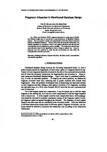
A. Embed the distributed database system in XML For packaging the file system associated with the finite element host (Table 1), the Extensible Markup Language (XML), which describes a class of data objects called XML documents, provides a useful approach (Figure 16) [5]. XML documents can contain both character data and markup. Markup encodes a description of the document's storage layout and logical structure. A Document Type Definition (DTD), a file separate from the main XML document (Figure 17), provides a set of rules for the XML document to which it is attached. The DTDs set the instructions for the structure of the XML document and define what elements are going to be used throughout the document. Hence, the DTD acts as a rule book that allows authors to create new documents of the same type and with the same characteristics as a base document [17, 28]. An XML processor reads XML documents and provides access to their content and structure.
2
Chapter IV Sections A and B constitute the second half of the paper, "Distributed, web-based microstructure database for brain tissue," Neurocomputing (2000), in press.
25
Table 1. File structure associated with a finite element host Type directory/file Root
Name
Contents
Root
Neuron subdirectory
Neuron label
FE universal FE location within brain address FE geometry file Hexahedron parameters Neuron subdirectories Neuron address Coordinates within the FE Soma geofile Soma synapse file
Dendritic segment subdirectory (level n)
Dendritic segment label
Dendritic segment subdirectories (level 1) Axonal segment subdirectories (level 1) Dendritic segment geofile
Dendritic segment synapse file
Axonal segment subdirectory (level m)
Axonal segment label
Daughter dendritic segment subdirectories (level n+1) Axonal segment geofile
Axonal segment synapse file
Daughter axonal segment subdirectories (level m +1)
Purpose
Position and orientation of soma within the FE For each synapse, identifies site of postsynaptic terminal and universal synaptic address of its associated presynaptic terminal
Initial position and orientation of segment (relative to segment at level n-1, length, diameter, taper, trajectory parameters, etc. For each synapse, identifies site of postsynaptic element and universal synaptic address of its associated presynaptic terminal
Initial position and orientation of segment (relative to segment at level m1, length, diameter, NURBS parameters, etc. For each synapse, identifies site of presynaptic terminal and universal synaptic address of its associated postsynaptic element
26
Figure 16. A processed XML document describing a hierarchical network data structure associated with a finite element host
27
]>
Figure 17. Root.dtd
B. Build a web-based graphical interface to gyri models XML provides information about the structure and content of documents, but leaves issues of document style and presentation to the software package used to parse and process it [29]. The markup governs content and structure, whereas associated style sheets govern how the content and structure are presented to the user. In order to build a web-based graphical interface to XML-based database (Figure 18), a set of style rules that define the attribute settings for each markup element is needed. Each style rule has
28
two parts: the selector and the declaration. The selector is the markup element to which the style rule is applied, whereas the declaration is specific information about how the element should be presented.
Figure 18. A formatted HTML document converted from the XML document shown in Figure 16 by a set of style rules
Embedding the distributed database system in XML not only provides structure but also adds flexibility in presenting information. An XML document may contain files
29
describing the morphology of a neuron, a rendering of a finite element model, or an interactive 3D-environment set in Virtual Reality Modeling Language (VRML) [2] or Java3D [31]. The style rules associated with the XML document facilitate presentation of different types of information in an XML browser. In addition, an XML browser allows a unified view of XML database documents distributed over the Web, paralleling the way an HTML browser sews together HTML documents distributed over the Web, and, therefore, adds web-accessibility to the distributed database system. A web-based graphical interface to the finite element models, using XML, enables a structured visualization of cortical gyri and provides access to the generated databases. When embedded in the graphical interface, Exploring the Brain Forest, a virtual reality environment set in VRML, coordinates an exploratory and interactive viewing environment for the human cerebral cortex. C. Treatment of partial neuronal information in a finite element host So far, we have only considered representing neuronal morphology cases whose soma, fibers and processes are all contained within a finite element host. However, other than synthetically generated neurons with such prior-constraints, it is unlikely that a neuron reconstructed from scanned blocks of tissue remains solely within one finite element host. Many of the neuronal processes reconstructed from a tissue block are likely to emanate from neurons whose somata reside in adjacent blocks (or finite elements). Some axonal fibers may be association fibers whose neurons have their soma in finite elements half way across the brain, and their exact finite element of origin is
30
probably not known. Accordingly, some methods to label fibers entering or leaving the finite element become necessary. Before labeling fibers entering or leaving the finite element, we extend our file structure associated with a finite element host to include 'ambiguous' segment subdirectories (Table 2). Ambiguous segments are neuronal fibers that are not yet distinguished as either dendritic or axonal. When additional information becomes available (such as the fiber's soma, the type of its parent segment, etc.), ambiguous segments can be reclassified as dendritic or axonal segments.
Table 2. Extended file structure associated with a finite element host Type directory/file Root
Name
Contents
Purpose
Root
FE universal address
FE location within brain Hexahedron parameters
FE geometry file Neuron subdirectories Neuron subdirectory
Neuron label
Ambiguous segment subdirectories Neuron address Soma geofile Soma synapse file Dendritic segment subdirectories (level 1) Axonal segment subdirectories (level 1)
Dendritic segment subdirectory (level n)
Dendritic segment label
Dendritic segment geofile
Dendritic segment synapse file
Coordinates within the FE
31
Table 2. Continued Type directory/file
Name
Contents
Purpose
(If an exiting segment,) - exiting segment label - entering segment label if known (If an entering segment,) - entering segment label
Axonal segment subdirectory (level m)
Axonal segment label
Daughter dendritic segment subdirectories (level n+1) Axonal segment geofile
Axonal segment synapse file (If an exiting segment,) - exiting segment label - corresponding entering segment label if known (If an entering segment,) - entering segment label
Ambiguous segment subdirectory (level n)
Ambiguous segment label
Daughter axonal segment subdirectories (level m +1) Ambiguous segment address
Coordinates within the FE
Segment geofile Segment synapse file (if an exiting segment) - exiting segment label - corresponding entering segment label (if an entering segment) - entering segment label Ambiguous segment subdirectories (level n+1)
Position and orientation of segment within the FE
32
For treatment of partial neuronal information, we assume that all fibers in a finite element model whose somata reside in it are traced, labeled, and stored in our finite element file structure. We consider two cases where the fibers' soma of origin is known and where it is not known. (1) Treatment of exiting and entering segments whose soma of origin is known By our assumption above, the exiting segment in this case is uniquely labeled, is classified as either dendritic or axonal, and contains all the relevant information associated with this segment as specified in our file structure table. We give this exiting segment a unique exiting segment label. In addition, we notice that this exiting segment is entering an adjacent finite element. We also uniquely label the entering segment and classify it as dendritic or axonal. Finally, we record the bi-directional link between two segments by storing the entering segment label with the associated exiting segment and the exiting segment label with the associated entering segment. (2) Treatment of exiting or entering segments whose soma of origin is not known Since the soma of origin is not known, this segment cannot be classified as exiting or entering upon encounter. Hence, we initially label this segment as both entering and exiting. When we find that this segment bifurcates or terminates in the finite element, we can reclassify it as an entering segment.
Similarly, it can be
reclassified as an exiting segment when more information becomes available based on the direction of biological growth. Initially, it may not be clear whether this segment is dendritic or axonal. Hence, we classify this segment as ambiguous. When its soma of
33
origin or the classification of its parent segment is known, the segment can be appropriately reclassified as dendritic or axonal. Next, we present a recursive algorithm that shows the overall structure of treating partial neuronal information in a finite element model. At any given stage of the reconstruction process in which we encounter partial neuronal morphology information, we keep a set of maximal subtrees. Each subtree stores the maximal partial neuronal information associated with its subtree root. The subtrees are merged as more information becomes available to ultimately yield the file structure for a neuron subdirectory in which they are the neuron's segment subdirectories.
Algorithm TracePartialNeurons Input: Neuronal morphology information in a finite element Output: File structure table associated with a finite element host 1. Identify all segments and store them in a set S 2. For each segment s in S 3.
Uniquely label s
4.
Classify s as both entering and exiting segment
5.
Classify s as ambiguous segment
6.
Mark s as a root and store it in the set R
7.
Delete s from S
8. For each root r in R 9.
Trace all fibers associated with r
34
10.
Merge r with its associated fibers and make bi-directional links between the parent and child segments
11.
if r can be classified as dendritic or axonal
12. 13. 14.
classify r and all the nodes in its subtree accordingly if r can be classified as entering or exiting classify it and its corresponding exiting/entering segment accordingly.
15. if more neuronal morphology information exists, call TracePartialNeurons
35
CHAPTER V
3D RECONSTRUCTION AND SIMULATED SECTIONING
A. 3D reconstruction of neurons Burton and McCormick described a fast automated system, called the Spaghetti Factory, for tracing neurons in parallel, adequate to support a quantitative analysis of neuron morphology [8, 10]. The system automates digitized neuron feature extraction and reconstruction, thereby replacing current largely manual techniques for tracing individual neurons. Serial sections of brain tissue are created by physical sectioning. Sections are processed during scanning to determine regions of interest (ROIs) and to quickly cull unnecessary image data. An aggressive data culling and compression scheme reduce the original volumetric data into an ROI-based image collection that makes temporary secondary storage feasible. Neighboring reconstructed segments created from these matches are disambiguated resulting in an abbreviated structural description of the tissue’s neurons and fiber tracts. The Spaghetti Factory provides the type conversion from brain tissue volume data to neuron/forests data (Figure 19): It literally “extrudes” volume data into parallel streams of neuronal segments and fibers, which are then reassembled into neuron/forest data. The ROIs of each tissue section serve as mobile “holes” in the extrusion plate [6]. The knowledge of what segments, fibers, and their bifurcations look like, modeling the
36
knowledge base of a trained microscopist, makes the automated reconstruction of neurons and their mutual connections possible. The forest of 3D reconstructed neurons is placed in the neuron/forest database, and therefore can be drawn upon to build virtual environments using Exploring the Brain Forest [7] visualization software.
Figure 19. Helix data set with 10 segments [6]
The Spaghetti Factory uses Section, Image, Segmenter, Contour, OBB, Segment, Reconstructor, and Point2i or Point2f objects to solve the reconstruction problem [6]. A Section object representing a tissue section stores the section's Z-position, thickness, corresponding digital image also stored in the Image object, and the list of feature Contours extracted from the image. The Segmenter algorithm object assigned to the Section performs image segmentation. The Contour object stores boundary points from a neuron segment intersection. The OBB (oriented bounding box) object determines a minimal, aligned rectangle that tightly bounds a Contour. The Segment object saves
37
points along each segment path during the segment tracing process. The Point2i and Point2f objects represent 2D points and provide distance measurements. Finally, the Reconstructor object implements the segment tracing algorithm and defines a basic interface for specific reconstruction algorithms. The reconstructed neuron is rendered as a wireframe model, with the original neuron geometry rendered in transparent cylinders, thereby creating a skeleton and skin model. B. Simulated sectioning Nslicer, a tool that simulates sectioned data from existing neuron models, reads existing descriptions of 3D neuron models and creates a digital image sequence of sectioned tissue. Nslicer is written in C++ and utilizes the OpenGL graphics library for rendering [35]. Nslicer builds a cylindrical representation of the neuron’s process after loading the neuron description file. 3D line segments, with each segment modeled by polygonal cylinders of 5 to 9 sides, represent neural processes. The polygons are saved into a callable OpenGL display list for ease of rendering. When the description is read, X, Y, and Z maxima and minima are recorded for configuring the graphics display and determining the bounds for the sectioning within a right-handed coordinate system. Once loaded, Nslicer sets the position to the maximum Z value, which is "in front" of the neurons from the camera's point of view. Sectioning is performed as the user moves a translucent thin line along the Z-axis from maximum (in front) to minimum (in back). OpenGL's front and back clipping planes are set close together, and the neuronal processes at each level of the line are rendered [6].
38
CHAPTER VI
SYNAPSE GENERATION AND IDENTIFICATION
The brain can be represented as a collection of interconnected neurons. Brain connectivity can be described at the level of volume-filling circuitry that records which neuron (and type) is the source of the axon, where the axonal arbor projects (into which pools of neurons) and for each of its axonal segments, ascertains the type and location of all its synapses on postsynaptic neurons. Connections are mediated through synapses [34]. A synapse is a connection between a presynaptic and a postsynaptic process (e.g., between a source axon and a target dendrite). Hence, each synapse can be cut and split into its pre- and post-synaptic terminals. These terminals are labeled with a universal synaptic address and then assigned respectively to their pre- and post-synaptic neurons. This information completely describes the neural connectivity of the tissue: its neural network can be reconstructed solely from a description of its individual neurons. A. Synapse generation In principle, the synaptology at a volume-filling circuitry level of detail of all neurons within a finite element can be estimated [23]. We can generate a synthetic forest of neurons filling the specified finite element, where the forest preserves the spatial distributions (layer-by-layer) and neuron morphologies observed within the finite element [22]. Then examining each synthetic neuron in turn, we evaluate the probability
39
that its soma (considered as a segment at level 0) and higher-level dendritic segments form potential synapses with neighboring fibers. These neighboring fibers, candidates for synapse formation, can be axonal segments of neighboring neurons, recurrent axon collaterals, or association fibers. For each fiber, there is a point of closest approach by a dendritic segment, and it is at this point that a synapse is most likely to form [25] (Figure 20). To complete the process, we need to invoke the "principle of the promiscuous neuron", to wit "if a dendrite and a fiber can form a more perfect union (a synapse), they will" [18]. Clearly the probability of a synaptic union drops off sharply with the intersegment distance r.
But within 1-4 µm, the probability of spines developing and
synapses forming is high [34].
Figure 20. Point of closest approach by a dendritic segment to an axial fiber (axon)
40
Kristine Harris, in her recent lapsed time video of synapse formation in cultured neurons [18], shows budding spines “groping” for one another. So, quite as growthbased modeling of neuron morphology is driven by knowledge of growth cone dynamics, the synaptology of brain tissue will be driven by knowledge of spine dynamics and the groping process by which synapses are formed. B. Build a distributed database system for the description of brain tissue Each neuron, as described in Chapter IV, is assigned to the finite element that contains its soma. It is convenient to consider a distributed database system wherein each finite element is implemented as an independent host. This host contains all structural information relevant to both the finite element and to the neurons it contains. The directory structure of this host (i.e., finite element) is described in Table 1 in Chapter IV. Of central importance is the description of the subdirectories associated with an individual neuron. The root directory of a neuron contains a collection of files describing the soma and subdirectories of all first-order dendritic or axonal segments.3 The synapse file associated with each soma, dendritic or axonal segment includes, for each synapse, the synapse name and the universal address of its associated postsynaptic (or presynaptic) terminal. These files carry the brain connectivity information, allowing one to reassemble the brain from its individual neurons. These putative synaptic links will usually be estimated by geometric modeling.
3
Formally it is convenient to treat the soma as a segment at level 0. The soma, unlike segments at other levels, uniquely allows subdirectories for both dendritic and axonal segments. Typically there are 5-10 first-order dendritic segments (each with its own subdirectory) and one first-order axonal segment (and hence subdirectory).
41
The interpretation is both natural and straightforward. Web pages are assigned to all files, and in particular, to the synapse files described in the distributed database system. The user, examining a given dendritic segment of the neuron, can open the synapse page for the segment and select a postsynaptic terminal. A mouse click links the user to the associated axonal segment page of the presynaptic neuron, and identifies the associated presynaptic terminal. Similar strategies can be applied to axonal segments and soma.
42
CHAPTER VII CONCLUSIONS A. Summary A database and interface system for brain tissue that supports organization and visualization of three types of brain tissue data -- volume data, neuron/forest data, and network data -- is proposed and prototyped. The cerebral cortex is partitioned into hexahedral finite elements, each of which hosts neuronal databases associated with it. A microstructure database system was established to organize individual neurons and to model local cortical microstructure by wiring up the neuronal forests. A prototype XML system that includes a DTD for each database element and a set of corresponding XSL [12] rules has been implemented to add structured visualization and web-accessibility of data. For the work reported in this thesis, the database stores 1 to 10 synthetically generated neurons with geometric constraints that require them to reside within finite elements that contain their soma. B. Future work Our distributed, microstructure database system can be extended to accommodate a large-scale empirical data set. A list of future improvements follows: 1. Fully incorporate the neuron visualizer and the Spaghetti Factory into the XML system. The neuron visualizer is written in C++ and interfaced with the FastLight ToolKit (FLTK) to run on SGI or PC platforms. The Spaghetti Factory is written in
43
C++ and vtk [30], and run on Linux. These two software systems need to be incorporated into the XML system to be web-accessible and to benefit from the structured information management and visualization offered by XML. When fully integrated, they add the functionalities to interactively read and edit the neuronal input files, to generate their 3D images, and to view their corresponding section image stacks, ROIs and VOIs. 2.
Extend the DTD and style rules for our XML system.
As step 1 above is
implemented, we need to expand our DTD and style rules to include more elements and attributes. 3. Model and match the afferent and efferent fibers of the finite elements. With the empirical data, we are bound to observe some fibers that enter or leave a finite element, where their soma of origin is not known. These fibers need to be recorded and matched together in order to effectively trace neurons from the volumetric data. 4. Estimate and implement synapses in our XML system.
Given empirical data,
candidates and their respective probabilities for synapse formation need to be efficiently calculated.
Once a synapse is identified, its pre- and post- synaptic
terminals are linked by a unique synaptic address and can be visualized in juxtaposition. 5.
Create geometric models of local cortical networks.
Once synapses are
systematically estimated, we need to create geometric models of local cortical microstructure to develop neuroanatomically based cortical circuit models that reconstruct the connectivity of the tissue and quantify its neural components.
44
REFERENCES [1]
M. Ackerman, Accessing the Visible Human Project, D-Lib Magazine (October 1995), http://www.dlib.org/dlib/october95/10ackerman.html.
[2]
A.L. Ames, D.R. Nadeau, J.L. Moreland, VRML 2.0 Sourcebook, 2nd Ed., John Wiley & Sons, Inc., New York, 1997.
[3]
D.A. Batte, Finite element decomposition and grid generation for brain modeling and visualization, MS Thesis, Department of Computer Science, Texas A&M University, 1997.
[4]
D.A. Batte, T.S. Chow, B.H. McCormick, Finite element decomposition of human neocortex, in: J.M. Bower (Ed.), Computational Neuroscience: Trends in Research, 1997, Plenum Press, New York, 1997, pp. 573-578.
[5] T. Bray, J. Paoli, and C. Sperberg-McQueen (Eds.), Extensible Markup Language (XML) 1.0, W3C Recommendation 10-Feb-98, 1998, http://www.w3.org/TR/1998/REC-xml-19980210. [6]
B.P. Burton, Automated 3D reconstruction of neuronal structures from serial sections, MS Thesis, Department of Computer Science, Texas A&M University, 1999.
[7]
B.P. Burton, T.S. Chow, A.T. Duchowski, W. Koh, B.H. McCormick, Exploring the brain forest, Neurocomputing 26-27 (1999) 971-980.
[8]
B.P. Burton, B.H. McCormick, Virtual Neurocomputing 26-27 (1999) 981-987.
[9]
K. Brodmann, Vergleichende Lolkalisationslehre der Grosshirnrinde, J. A. Barth, Leipzig, 1909.
microscopy
of
brain
tissue,
[10] G.J. Carman, H.A. Drury, D.C. Van Essen, Computational methods for reconstructing and unfolding the cerebral cortex, Cereb Cortex Nov-Dec;5(6) (1995) 506-517. [11] S. Chow, Finite element decomposition of the human neocortex, MS Thesis, Department of Computer Science, Texas A&M University, 1998. [12] S. Deach (Ed.), Extensible Stylesheet Language (XSL) Specification, W3C Working Draft 21-APR-99, 1999, http://www.w3c.org/TR/WD-xsl.
45
[13] R.W. DeVaul, B.H. McCormick, Neuron developmental modeling and structural representation 1. an introduction to the N++ language, an open stochastic L-system. Technical Report, Scientific Visualization Laboratory, Department of Computer Science, Texas A&M University, College Station, TX, December, 1996. [14] P. Dierckx, Curve and Surface Fitting with Splines, Clarendon Press, Oxford, 1995. [15] H. Drury, D. Van Essen, C. Anderson, C. Lee, T. Coogan, J. Lewis, Computerized mappings of the cerebral cortex: a multiresolution flattening method and a surfacebased coordinate system, Journal of Cognitive Neuroscience 8 (1) (1996) 1-28. [16] G. Farin, Curves and Surfaces for CAGD, 4th Ed., Academic Press, Inc., San Diego, CA, 1996. [17] C.F. Goldfarb, P. Prescod, The XML Handbook, Prentice Hall PTR, Upper Saddle River, NJ, 1998. [18] K. Harris, Video presentation, Society for Neuroscience Conference, Los Angeles, CA, 1998. [19] P. Knupp, S. Steinberg, Fundamentals of Grid Generation, CRC Press, Boca Raton, FL, 1994. [20] B.H. McCormick, Design of a brain tissue scanner, Neurocomputing 26-27 (1999) 1025-1032. [21] B.H. McCormick, R.W. DeVaul, Neuron developmental modeling and structural representation 2. the stochastic model, Technical Report, Scientific Visualization Laboratory, Department of Computer Science, Texas A&M University, College Station, TX, 1996. [22] B.H. McCormick, R.W. DeVaul, W.R. Shankle, J.H. Fallon, Modeling neuron spatial distribution and morphology in developing human cerebral cortex, Neurocomputing (2000), in press. [23] B.H. McCormick, W. Koh, W.R. Shankle, J.H. Fallon, Geometric modeling of local cortical circuitry, Neurocomputing (2000), in press. [24] B.H. McCormick, K. Mulchandani, L-system modeling of neurons, Proc. Visualization in Biomedical Computing, SPIE 2359 (1994) 693-705.
46
[25] B.H. McCormick, G.T. Prusky, S. Tewari, Stochastic modeling of the pyramidal cell modules, in: J.M. Bower (Ed.), Computational Neuroscience: Trends in Research, 1997, Plenum Press, New York, 1997, pp. 129-134. [26] K. Mulchandani, Morphological modeling of neurons, MS Thesis, Department of Computer Science, Texas A&M University, 1995. [27] National Library of Medicine, Fact sheet: the Visible Human Project, August 1999, http://www.nlm.nih.gov/pubs/factsheets/visible_human.html. [28] W.J. Pardi, XML in Action, Microsoft Press, Redmond, WA, 1999. [29] N. Pitts-Moultis, C. Kirk, XML Black Book, Coriolis Group, Albany, NY, 1999. [30] W. Schroeder, K. Martin, Lorensen, The Visualization Toolkit, 2nd Ed., Prentice Hall PTR, Upper Saddle River, NJ, 1998. [31] H. Sowizral, K. Rushforth, M. Deering, Java3D API Specification, Sun Microsystems Inc, December 1998, http://java.sun.com/products/javamedia/3D/forDevelopers/j3dguide/j3dTOC.doc.html. [32] J.F. Thompson, B.K. Soni, N.P. Weatherill, Handbook of Grid Generation, CRC Press, Boca Raton, FL, 1999. [33] C. Von Economo, The Cytoarchitectonics of the Human Cerebral Cortex, Oxford Univ. Press, Oxford, 1929. [34] E.L. White, Cortical Circuits: Synaptic Organization of the Cerebral Cortex Structure, Function, and Theory, Birkhauser, Boston, 1989. [35] M. Woo, J. Nieder, T. Davis, OpenGL Programming Guide, Addison-Wesley Developers Press, Reading, MA, 1997.