Diverse and Proportional Size-l Object Summaries for Keyword Search Georgios J. Fakas
Zhi Cai
Nikos Mamoulis
Department of Computer Science and Engineering HKUST Hong Kong
College of Computer Science Beijing University of Technology Beijing, China
Department of Computer Science The University of Hong Kong Hong Kong
[email protected]
[email protected]
[email protected]
ABSTRACT The abundance and ubiquity of graphs (e.g., Online Social Networks such as Google+ and Facebook; bibliographic graphs such as DBLP) necessitates the effective and efficient search over them. Given a set of keywords that can identify a Data Subject (DS), a recently proposed relational keyword search paradigm produces, as a query result, a set of Object Summaries (OSs). An OS is a tree structure rooted at the DS node (i.e., a tuple containing the keywords) with surrounding nodes that summarize all data held on the graph about the DS. OS snippets, denoted as size-l OSs, have also been investigated. Size-l OSs are partial OSs containing l nodes such that the summation of their importance scores results in the maximum possible total score. However, the set of nodes that maximize the total importance score may result in an uninformative size-l OSs, as very important nodes may be repeated in it, dominating other representative information. In view of this limitation, in this paper we investigate the effective and efficient generation of two novel types of OS snippets, i.e. diverse and proportional sizel OSs, denoted as DSize-l and PSize-l OSs. Namely, apart from the importance of each node, we also consider its frequency in the OS and its repetitions in the snippets. We conduct an extensive evaluation on two real graphs (DBLP and Google+). We verify effectiveness by collecting user feedback, e.g. by asking DBLP authors (i.e. the DSs themselves) to evaluate our results. In addition, we verify the efficiency of our algorithms and evaluate the quality of the snippets that they produce.
1.
INTRODUCTION
Keyword search on the web (W-KwS) has dominated our lives, as it facilitates users to find easily and effectively information using only keywords. For instance, the result for query Q1 =“Faloutsos” consists of a set of links to web pages containing the keyword(s) together with their respective snippets. Snippets are short fragments of text extracted from the search results (e.g., web pages); they significantly enhance the usability of search results as they provide an intuition about which results are worth accessing and which can be ignored. Furthermore, snippets may provide the complete answer Permission to make digital or hard copies of all or part of this work for personal or classroom use is granted without fee provided that copies are not made or distributed for profit or commercial advantage and that copies bear this notice and the full citation on the first page. Copyrights for components of this work owned by others than ACM must be honored. Abstracting with credit is permitted. To copy otherwise, or republish, to post on servers or to redistribute to lists, requires prior specific permission and/or a fee. Request permissions from
[email protected]. SIGMOD’15, May 31–June 4, 2015, Melbourne, Victoria, Australia. c 2015 ACM 978-1-4503-2758-9/15/05 ...$15.00. Copyright http://dx.doi.org/10.1145/2723372.2737783.
E XAMPLE 1. The OS for Michalis Faloutsos Author: Michalis Faloutsos ...Paper: On Power-law Relationalships of the Internet Topology. ......Conference: SIGCOMM. Year: 1999. ......Co-Author(s): Christos Faloutsos, Petros Faloutsos. ......Cites: Building Shared..., ...Cited by: The Structure..., ...Paper: BLINC: Multilevel Traffic Classification in the Dark. ......Conference: ACM SIGCOMM Computer Comm. Review Year:2005. ......Co-Author(s): T. Karagiannis, K. Papagiannaki. ......Cites: A Parametrizable methodology..., ...Cited by: P4P: Provider..., ...Paper: Transport Layer Identification of P2P Traffic. ......Conference: SIGCOMM. Year:2004. ......Co-Author(s): T. Karagiannis, A. Broido. ......Cites: Their Share: Diversity..., Cited by: Internet Traffic...... ... ...
to the searcher’s actual information needs (if, for example, the user is only interested in whether Michalis Faloutsos is a Professor), thus preventing the need to retrieve the actual result [27]. The keyword search paradigm has also been introduced in relational databases (R-KwS) (e.g., [19]). According to the R-KwS paradigm, we search for networks of tuples connected via foreign key links that collectively contain the keywords. For example, the query “Faloutsos”+“Agrawal” over the DBLP database returns tuples Faloutsos and Agrawal from the Author table and their associations through co-authored papers. However, the R-KwS paradigm may not be very effective when searching information about a particular data subject (DS) (e.g., Faloutsos and his papers, co-authors, etc.), because it only returns tuples containing the keywords (in this case only Faloutsos Author tuples). Hence, R-KwS fails to address search for the context of most important tuples around a central tuple (i.e., DS). In view of this, in [12], the concept of object summary (OS) was introduced; an OS summarizes all data held in a database about a particular DS, searched by some keyword(s). More precisely, an OS is a tree with the tuple nDS containing the keywords (e.g., Author tuple M. Faloutsos) as the root node and its neighboring tuples, containing additional information (e.g., his papers, co-authors etc.), as child or descendant nodes. The precise definition of an OS is discussed in Section 2; in a nutshell, a tuple is included in the OS if it is of high importance (based on link properties in the tuple network graph of the database) and it is connected to nDS via a short path. For instance, the result for Q1 is a set of OSs: one for each Faloutsos brother. Example 1 illustrates the OS for Michalis (the complete set of papers and the OSs of the other two brothers are omitted due to lack of space). Note that the OS paradigm is in more analogy to the W-KwS paradigm, compared to R-KwS paradigm. For instance, Example 1 resembles a web page (as both include comprehensive information about the DS). Therefore, for the non-technical users with experience only on W-KwS, the OS paradigm will be friendlier and also closer to their expectations.
E XAMPLE 2. The size-15 OS for Michalis Faloutsos Author: Michalis Faloutsos ...Paper: On Power-law Relationalships of the Internet Topology. ......Co-Author: Christos Faloutsos,... ...Paper: Power Laws and the AS-Level Internet Topology. ......Co-Author: Christos Faloutsos,... ...Paper: ACM SIGCOMM‘ 99. ......Co-Author: Christos Faloutsos,... ...Paper: Information survival thr.... .Co-Author: Christos Faloutsos,... ...Paper: The Connectivity and Fault... .Co-Author: Christos Faloutsos,... ...Paper: BGP-lens: Patterns and An... .Co-Author: Christos Faloutsos,... ...Paper: The eBay Graph: How Do.... .Co-Author: Christos Faloutsos,... E XAMPLE 3. The DSize-15 OS for Michalis Faloutsos Author: Michalis Faloutsos ...Paper: On Power-law Relationalships of the Internet Topology. .......Conference: SIGCOMM. Year: 1999. .......Co-Author: Christos Faloutsos, .... ...Paper: Information Survival Threshold in Sensor and P2P Networks. ......Co-Author: S. Madden, ..., Conference: INFOCOM. ...Paper: Power Laws and the AS-Level Internet Topology. .......Conference: IEEE/ACM Tr. Netw. Year: 2003. .......Co-Author: Christos Faloutsos,.. ...Paper: Network Monitoring Using Traffic Dispersion Graphs. ......Co-Author: M. Mitzenmacher, ...Conference: SIGCOMM.
E XAMPLE 4. The PSize-15 OS for Michalis Faloutsos Author: Michalis Faloutsos ...Paper: On Power-law Relationalships of the Internet Topology. .......Conference: SIGCOMM. Year: 1999. .......Co-Author: Christos Faloutsos, .... ...Paper: Denial of Service Attacks at the MAC Layer... ......Co-Author: S. Krishnamurthy, ..., Conference: MILCOM. ...Paper: Power Laws and the AS-Level Internet Topology. .......Conference: IEEE/ACM Tr. Netw. .......Co-Author: Christos Faloutsos,.. ...Paper: Reducing Large Internet Topologies for Faster Simulations ......Co-Author: S. Krishnamurthy, L. Cui,...Conference: NETWORKING.
In general, an OS is a concise summary of the context around any pivot database tuple or graph node, finding application in (interactive) data exploration, schema extraction, etc. (e.g., [16]). Another application of this summarization concept is on semantic knowledge graphs [25, 6]. In [14, 15], OS snippets are proposed (denoted as size-l OSs); size-l OSs are composed of only the l most important nodes. Example 2 illustrates the size-l OS for M. Faloutsos with l = 15 on the DBLP database. According to [14, 15], a size-l OS should be a standalone sub-graph of the complete OS, composed of the l most important nodes only, so that the user can comprehend it without any additional information. For this reason, the l nodes should form a connected graph that includes the root of the OS (i.e., nDS ). To distinguish the importance of an individual node ni to be included in a size-l OS, a local importance score (denoted as li(ni )) is defined. Based on the local importance scores of the nodes of an OS, we can find the partial OS of size l with the maximum importance score. However, this selection criterion (i.e., maximizing importance score) can render such snippets ineffective. For instance, in Example 2, the co-authorship of Michalis with Christos Faloutsos, who is a very important author monopolizes the snippet with papers coauthored only with Christos. Thus, we argue that the diversity of constituent nodes will improve the snippet’s effectiveness. In addition, we argue that frequent appearances of nodes in an OS should also be proportionally represented in an effective snippet. Hence, in this paper we propose two novel snippets, namely diverse and proportional size-l OSs denoted as DSize-l OS and PSize-l OS respectively. More precisely, in a DSize-l OS we favor diversity by penalizing repetitions of nodes, whereas, in a PSize-l OS, we favor proportionality, i.e., a frequent node should be analogously represented, facilitating diversity at the same time. For instance, the
DSize-l OS of Example 3 includes C. Faloutsos only twice, allowing the appearance of other important co-authors as well. Similarly, the PSize-l OS of Example 4 includes also frequent co-authors S. Krishnamurthy and L. Cui who do not appear at all in the DSizel OS. To compute them, we calculate a combined score per node, which integrates (1) importance, (2) affinity to the data subject node nDS and (3) diversity or proportionality. The efficient generation of DSize-l or PSize-l OSs is a challenging problem since information about the repetitions and frequencies of nodes is required and incremental computation is not possible (as opposed to the original size-l OS computation problem [14]). We propose a brute force algorithm, BF-l, that produces optimal solutions but scales badly. Then, we propose a greedy algorithm (LASP) and its optimization (2-LASP). Both algorithms are general and can address both DSize-l and PSize-l OS snippet types (with minor modifications). In addition, we propose two preprocessing techniques for the two snippet types (PPrelim-l and DPrelim-l, respectively) that prune the input OSs before processing them. We conducted an extensive experimental study on the DBLP bibliographic and Google+ social network datasets. We verify effectiveness by collecting user feedback, e.g., by asking DBLP authors (i.e., the DSs themselves) to evaluate our size-l OSs. The users suggested that the results produced by our method are very close to their expectations and they are more usable than the respective size-ls OSs, which disregard diversity. In addition, we investigated in detail and verified the efficiency and approximation quality of our algorithms. The contributions of this paper can be summarized as follows: (1) the introduction of two novel OS snippets, DSize-l and PSizel OS, which capture diversity and proportionality respectively; (2) the introduction of a brute force algorithm and efficient greedy algorithms for their generation; (3) an extensive experimental evaluation that verifies the proposed methodologies. The rest of the paper is structured as follows. Section 2 describes background and related work. Section 3 describes the semantics of DSize-l and PSize-l OSs. Sections 4 and 5 introduce the optimal and greedy algorithms respectively, whereas Section 6 introduces preprocessing algorithms for DSize-l and PSize-l OS computation. Section 7 presents experimental results. Finally, Section 8 provides concluding remarks.
2.
BACKGROUND AND RELATED WORK
In this section, we first describe the concepts object summary (OS) and size-l OS, which we build upon in this paper. We then present related work in R-KwS, ranking, and summarization. To the best of our knowledge, no previous work has focused on the computation of diverse and proportional size-l OSs.
2.1
Object Summaries
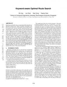
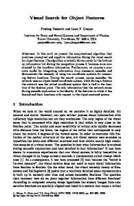
According to the keyword search paradigm of [11, 12], an object summary (OS) is generated for each node (tuple) nDS found in a graph (database) that contains the query keyword(s) (e.g., “Michalis Faloutsos” node of Author relation in the DBLP database1 ). An OS is a tree structure having nDS as a root and its neighboring nodes (i.e., those associated through foreign keys) as its children/descendant nodes. To construct the OSs, the relations which may hold the queried Data Subjects (DSs), denoted as RDS (e.g., the Author relation), and the relations linked around RDS are used. For each RDS , a Data Subject Schema Graph GDS is generated. Figure 2 illustrates the GDS for the Author relation of the DBLP database, whose schema is shown in Figure 1. A GDS is a directed labeled tree with 1
www.informatik.uni-trier.de/∼ley/db/
Author (1) 1.05, 7.38, 1, 1
Conference
ConfYear
Paper
Author
(1), 1,1
Figure 1: The DBLP Database Schema a fixed maximum depth that has an RDS as a root node and captures the subset of the schema surrounding RDS ; any surrounding relations participating in loop or many to many relationships are replicated accordingly. Namely, a GDS is a “treelization” of the schema graph, where RDS becomes the root, RDS ’s neighboring relations become child nodes and so on. Any looped and many to many relationships are replicated. Each relation in GDS is also annotated with statistical information that we describe later together with our methods. In order to generate an OS, the relations from GDS , which have high affinity with RDS are accessed and joined. The affinity of a relation Ri to RDS can be calculated by the formula: X af (Ri ) = wj mj · af (RParent ), (1) j
where j ranges over a set of metrics (m1 , m2 , . . . , mn ) and their corresponding weights (w1 , w2 , . . . , wn ), and af (RParent ) is the affinity of Ri ’s parent to RDS . The metrics’ scores range in [0, 1] and the corresponding weights sum to 1; thus, the affinity score of a node is monotonically non-increasing with respect to the node’s parent. More precisely we use four metrics: m1 considers the distance of Ri to RDS , i.e., the shorter the distance the bigger the affinity between the two relations. The remaining metrics consider the connectivity of Ri on both the database schema and data-graph. m2 measures the relative cardinality, i.e., the average number of tuples of Ri that are connected with each tuple in RP arent whereas m3 measures their reverse relative cardinality, i.e., the average number of tuples of RP arent that are connected with a tuple in Ri . m4 considers the schema connectivity of Ri (i.e., the number of relations it is connected to in the relation graph). Given an affinity threshold θ, a subset of GDS can be produced. Given a node (tuple) nDS in RDS , by traversing the GDS (e.g., by joining the corresponding relations) we can generate the OSs (Algorithm 4). For instance, for Q1 =“Faloutsos”, and for nDS =“Michalis Faloutsos” in the Author RDS of the DBLP database, the OS presented in Example 1 will be generated. Every tuple vi in the database carries a global importance weight gi(vi ), calculated using PageRank-inspired measures such as ObjectRank [3, 28] and ValueRank [13]. Due to the “treelization” of the schema graph by GDS , multiple tuples in an OS may correspond to the same tuple in the database. For instance, the same co-author (e.g., Christos Faloutsos) may appear multiple times (e.g., 12) in the OS of Michalis. Formally, for a node n of an OS, we use function g(n) to denote the corresponding tuple v in the database. Thus, for two OS nodes ni and nj , we may have g(ni ) = g(nj ) = v. We also denote as f r(v) (i.e., f r(g(ni ), or simply f r(ni )) the frequency of v in the given OS.
2.2
Size-l OSs
According to [14], given an OS and an integer l, a candidate sizel OS is any subset of the OS composed of l nodes, such that all l nodes are connected with nDS . The authors in [14] argue that a good size-l OS should be a standalone and meaningful synopsis of the most important and representative information about the particular DS (so that users can understand it as is, without any additional nodes). In particular, any intermediate nodes that connect nDS (e.g., M. Faloutsos) with other important nodes (e.g., C. Faloutsos) in the
Paper (0.92) 8.82, 7.38, 1, c(Paper) (33), 1, ( ) max(nDS)=0.6
PaperCitedBy(0.77) 7.38, 0, ∞→c(Paper), ( )
PaperCites (0.77) 7.38, 0, ∞→c(Paper), ( )
ConfYear (0.83) 0.84, 0.22, ∞→c(Paper),c(Paper)
( ), 33, 21
( ), 33, 21
(33), 33, 21
Co-author (0.82) 0.86, 0, ∞→c(Paper), ( ) ( ), 33, 21 mw(nDS)=0.7 mFr(nDS)=21
Conference(0.78) 0.22, 0, ∞→c(Paper), () ( ), 33, 21
DS
Figure 2: The DBLP Author G s, annotated with relation indexes: (affinity), max(Ri ), mmax(Ri ), UBFr(Ri ), c(Ri ), and exemplary nDS indexes: (c(Ri )), UBFr(Ri , mF r(nDS )) size-l OS guarantee that the size-l remains standalone, since these connecting nodes (e.g., co-authored papers) include the semantics of the associations. For instance, in Example 2, if we exclude paper “On Power-law . . . ” but only include the co-authors, we exclude the semantic association between nDS and co-author(s), which in this case is their common paper. The holistic importance PIm(Sl) of any candidate size-l OS Sl is defined as Im(Sl) = ni ∈Sl li(ni ), where li(ni ) = af (ni ) · gi(ni ). The affinity af (ni ) of a node ni equals the affinity of the relation where ni belongs (Eq. 1); the global importance gi(ni ) was defined in Section 2.1. A candidate size-l OS is an optimal size-l OS, if it has the maximum Im(Sl) over all candidate size-l OSs. The generation of a size-l OS is a challenging task because we need to select l nodes that are connected to nDS and at the same time result in the maximum score. An optimal dynamic programming algorithm (requiring O(nl2 ) time where n is the amount of nodes in the OS) and greedy algorithms were proposed in [14].
2.3
Keyword Search and Ranking
R-KwS paradigms facilitate the discovery of joining tuples (i.e., Minimal Total Join Networks of Tuples (MTJNTs) [19]) that collectively contain all query keywords and are associated through their keys; hence the concept of candidate networks is introduced (e.g., DISCOVER [19, 18]). R-KwS paradigms differ from OSs semantically, since they search for connections of keywords. Précis Queries [22, 24] resemble size-l OSs as they append additional information to the nodes containing the keywords, by considering neighboring relations. However, a précis query result is a logical subset of the original database (see [12] for a detailed comparison to size-l OSs). Other works in this context also investigate indexing and ranking techniques to facilitate efficiency [23]. Related ranking paradigms consider Importance, which weights the authority flow through relationships (e.g., ObjectRank [3, 28], ValueRank [13], PageRank [4], etc.) In this work we use nodes’ importance to model gi and more precisely global ObjectRank (for DBLP). Our algorithms are orthogonal to how importance of nodes is defined (alternative methods could also be investigated). Document Summarization. Web snippets [26, 27, 20] are examples of document summaries that accompany search results of W-KwSs in order to facilitate their quick preview. They can be
Table 1: Authors (ranked in descending pw[1] order) Name
li
fr
S.Krishnamurthy C.Faloutsos J.Cui T.Karagiannis M.Mitzenmacher G.Varghese K.Papagiannaki S.Madden M.Chrobak J.Eriksson
0.6 1.8 0.8 0.7 1.4 1.4 0.6 1.6 0.3 0.2
37 12 11 10 3 2 4 1 4 7
pq[1] pw[1] pq[2] pw[2] dv[1] dw[1] dv[2] dw[2] 12.3 4.0 3.7 3.3 1.0 0.7 1.3 0.3 1.3 2.3
7.4 7.2 3.0 2.3 1.4 0.9 0.8 0.5 0.4 0.4
7.4 2.4 2.2 2.0 0.6 0.4 0.8 0.2 0.8 1.4
4.4 4.3 1.8 1.4 0.8 0.6 0.5 0.3 0.2 0.2
1.0 1.0 1.0 1.0 1.0 1.0 1.0 1.0 1.0 1.0
0.6 1.8 0.8 0.7 1.4 1.4 0.6 1.6 0.3 0.2
0.9 0.9 0.9 0.9 0.9 0.9 0.9 0.9 0.9 0.9
0.5 1.6 0.7 0.6 1.2 1.2 0.5 1.4 0.3 0.1
either static (e.g., the first words of the document or metadata) or query-biased (e.g., containing the query keywords). However, the direct application of such techniques on OSs and databases in general is ineffective as they disregard the relational associations (e.g., for Q1, papers authored by Faloutsos will be disregarded as they do not include the "Faloutsos" keyword).
2.4
Diversity
Diversification of query results has attracted a lot of attention recently as a method for improving the quality of results by balancing similarity (relevance) to a query q and dissimilarity among results. Typically, given a query q and a desired number of results k, firstly we get a ranked list of results S in descending order of their similarity sim(si , q) to q. Then, the objective of diversification is to find a subset of S, R ⊆ S of size k, such that the elements in R are similar to q (w.r.t sim(q, si )) and at the same time dissimilar to each other (w.r.t. dis(si , sj )). The definition of sim and dis scores is orthogonal to the diversification problem per se and a variety of IR-based or probabilistic approaches have been used to define such functions (e.g., PageRank-based similarity). In most cases, the same function is used to estimate both scores (i.e., dis(si , sj ) = 1−sim(si , sj )). One of the earliest and most influential diversification functions is Maximal Marginal Relevance (MMR) [5], which trades off between the novelty (a measure of diversity) and relevance of search results; a parameter is used to control this trade off. A general framework for result diversification appears in [17] with eight axioms. In [17, 29], max-sum and max-min mono-objective objective functions and algorithms are proposed. Our proposed diversity definition is inspired by this mono-objective approach, where for each document, a single score trades off the relevance to the query and the dissimilarity from other documents. In [1, 2], probabilistic interpretations of sim and dis functions and objective functions are proposed. In [9, 10], an intuitive definition of diversity, called DisC diversity, is proposed where the computed diverse subset R covers all elements of S in the sense that for element in S there should be a similar element in R and at the same time the elements in R are dissimilar to each other (i.e., diversity). In [21], LogRank is proposed, a principled authority-flow based algorithm that computes a representative summary of the user’s activities by selecting activities that are simultaneously important, diverse and time-dispersed. Proportionality. [30, 8, 7] investigate proportional diversification. More precisely, in [8] an election-based method is proposed to address the problem of diversifying searched results proportionally (our work is inspired by this approach). However, this method disregards the similarity (or importance) of the computed set R to the query q and thus may result in including irrelevant objects into R. In [30], this limitation is addressed by considering relevance in the objective function. Differences. Our problem has two significant differences from the existing related works that renders their straightforward application inappropriate. (1) Related work considers diversifying a set
of mutually independent results (i.e., S and R sets) whereas we aim at finding an l-sized connected subtree of the OS, which is required to include the root nDS . (2) Previous work considers intervalscaled pairwise dissimilarity of elements (i.e., each element si ∈ S has a degree of dissimilarity to any other element sj ∈ S) whereas in our problem the dissimilarity between nodes is binary, i.e., OS nodes are either equal or not (i.e., either g(ni ) = g(nj ) or g(ni ) 6= g(nk )).
3.
DSIZE-L AND PSIZE-L SNIPPETS
We propose two types of size-l OSs, namely diverse DSize-l OSs and proportional PSize-l OSs, which extend the size-l OS definition [14] to capture diversity and proportionality, respectively. Similarly to size-l OSs, both DSize-l OSs and PSize-l OSs should be standalone sub-trees of the OS, composed of l important and representative nodes only, so that the user can understand them without any additional information. Thus, the l nodes should form a connected graph that includes the root of the OS (i.e., nDS ). We argue that an an effective DSize-l (PSize-l) OS should gracefully combine diversity (proportionality) and the local importance scores of constituent nodes. Hence, we propose that for each OS node ni , we estimate a respective score for diversity, proportionality, and local importance, denoted by dv(ni ), pq(ni ) and li(ni ), respectively. dv(ni ) (pq(ni )) and li(ni ) are combined to a single score dw(ni ) (pw(ni )) for a DSize-l (PSize-l) OS, simply denoted by w(ni ) when the context (i.e., diversity or proportionality) is clear. Then, the objective is to select the l nodes that (1) include nDS and form a connected subtree of the OS and (2) their sum of their w scores is maximized. Local importance (i.e., li(ni )) can be calculated as in the original size-l OS problem (i.e., by multiplying affinity with global importance [14]), thus hereby we discuss only diversity and proportionality. Recall that each OS node corresponds a single graph node (i.e., tuple) and that two different OS nodes may either correspond to the same tuple (e.g., g(ni ) = g(nj ) = v) or to different ones (e.g., g(ni ) 6= g(nj )) and this is the only criterion for their similarity. We do not consider the textual similarity among nodes, because this restricts the generality of our problem. For instance, although we can define similarity between papers (e.g., “On Power-law relationships of the Internet Topology” vs. “Power laws and the ASLevel Internet topology”) meaningfully, it does not make sense to define similarity between authors (e.g., “Chen” vs. “Cheng”). By considering categorical similarity only, we signify the importance of frequent nodes regardless their respective local importance.
3.1
Diversity (DSize-l OSs)
We suggest that the l nodes should be diversified by preventing the domination of very important nodes. For example, in the Michalis Faloutsos OS, the co-authorship with the very important author Christos Faloutsos dominates the snippet and this renders the snippet not representative. A natural criterion objective towards measuring diversity is to maximize the sum of dissimilarities between nodes. Thus, for a given graph node we suggest to estimate diversity as follows:
dv(ni ) = 1−
X nj ∈S,ni 6=nj
z(g(ni )) − 1 sim(ni , nj ) = 1− , (2) l−1 l−1
where sim(ni , nj )=1 if g(ni ) = g(nj ) or 0 otherwise; therefore the summation of similar nodes for ni in a snippet is z(g(ni )) − 1, where z(g(ni )) is the amount of times g(ni ) appears in the snippet. Dividing by l − 1, we normalize dv(ni ) in the range [0,1]. We also
denote as dv[z] the diversity for any node considering it appears z times in the snippet. For instance, for all nodes appearing only once, dv[1] = 1. As another example, consider l = 10 and that C. 2−1 = 98 = Faloutsos appears 2 times (i.e., z =2); dv[2] = 1 − 10−1 0.89 (Table 1). Note that this score corresponds to the graph node g(ni ); thus, both nodes will have the same dv, i.e 0.89 (an alterative way would be to score the first occurrence as 1 and the second as 0.78, since 1+0.78=0.89+0.89). This equation is inspired by (1) max-sum diversification that maximizes the sum of the relevance and dissimilarity of a set and by (2) the use of a mono-objective formulation, which, similarly to our equation, combines relevance and dissimilarity to a single value for each document [17]. Note that, in general, diversification approaches trade off (1) the similarity of results with the given query and (2) the dissimilarity among such results using a similarity measure (e.g., IR techniques). For instance, given a query “Internet Topology”, papers “On Power-law relationships of the Internet Topology” and “Power laws and the AS-Level Internet topology” have some similarity to this query but they also have some similarity among them; both types can be estimated using a common IR metric. This is not the case here, since (1) we do not have a similarity of nodes to the query but a local importance score in relation to nDS and (2) the similarity among nodes is categorical. Thus, local importance and categorical similarity are not meaningfully comparable. Note also that their respective values may not be in the same range (e.g., local importance may range in [0,10] whereas dv always ranges in [0,1]). Hence, unlike most diversification approaches, in the combining function dw(.) (to be defined in Section 3.3) we do not sum up local importance and dissimilarity, but multiply them.
3.2
Proportionality (PSize-l OSs)
We observe that in an OS we often find graph nodes (i.e., database tuples) multiple times. For instance, in the Michalis Faloutsos OS (see Table 1), we have 37 instances of S. Krishnamurthy, 12 instances of C. Faloutsos, 18 papers in INFOCOM, etc. We denote the frequency of a graph node v in an OS as f r(v) (or simply by f r when the context is clear). Graph nodes that appear in an OS multiple times could sometimes be comparatively weak in terms of importance, but still given their frequency in the OS, they should be represented analogously in an effective snippet. Thus, we suggest that in a PSize-l snippet, disregarding local importance (i.e., assuming that all nodes have the same li), we should include nodes in proportion of their frequency. For example, if a graph node v appears 37 times in the total of 1,259 OS nodes, then v should ideally appear bl·37/1, 259c times in the respective PSize-l OS. (Note that this may not practically possible as in-between nodes may also be required, i.e., the co-authored papers in our example.) Since l is small in size, we need some incremental selection policy to cover proportionally the different frequent sets; namely, at each iteration we can append a different frequent node (facilitating to some extend a round-robin selection). For this purpose, we propose the use of the proportional quotient as follows: pq(ni ) =
f r(g(ni )) , α · z(g(ni )) + 1
(3)
where z(g(ni )) is the times that the node ni is about to be added in the snippet (i.e., it has already been added z-1 times), f r(g(ni )) is the frequency that the node appears in the OS and α is a constant that can tune proportionality. This equation is inspired by the Sainte-Laguë Algorithm [8] (with α = 2) and empirically we found that it is very effective for our problem (other equations can also be considered, e.g., [7, 30]). For a given z value, i.e., a given z(g(ni )), we denote the respective quotient as pq(ni )[z]. The ra-
tionale of this quotient is to favor a frequent node and each time a node is added to the snippet its pq(ni )[z] score is significantly decayed so that other frequent items will be selected, in turn. This way diversification is also facilitated. For instance, considering f r = 12 and α = 2 for C. Faloutsos, by adding this node for the first time we get pq[1] = 12/3 = 4 and for the second time we get pq[2] = 12/5 = 2.4. Nodes Addition Order Criterion. Note that the order we consider adding a node determines the respective pq(ni )[z] and thus the aggregate score of a PSize-l OS P Sl. Thus we choose to add them in the order that maximizes the holistic Im(P Sl) score (Equation 5; to be defined in Section 3.3). For instance, consider OS nodes ni and nj with g(ni ) = g(nj ); if we add ni first, we get pq(ni )[1] that will result to the aggregate score Im(P Sl1 ); if we add nj first, we get pq(nj )[1] and respective aggregate Im(P Sl2 ) score. Therefore, we choose the order that will result to the largest aggregate score (i.e., arg max( Im(P Sl1 ), Im(P Sl2 ))). Note that we need this constraint as otherwise we may not get deterministic aggregate score (i.e., the same PSize-l OS may produce different scores depending the order we consider to append nodes).
3.3
DSize-l and PSize-l Definitions
Based on the above discussion, for DSize-l OSs, we propose the following combining score per node: dw(ni ) = li(ni ) · dv(ni ),
(4)
where li(ni ) = af (ni ) · gi(ni ) is the local importance of ni and dv is the diversity factor (Equation 2). Table 1 depicts examples of how these scores can be obtained by constituent scores for l =10. For instance, consider the simplified example where we need to select 5 authors (and thus an intermediary paper), then we will select twice C. Faloutsos (i.e., 0.89*1.8+0.89*1.8=1*1.8+0.78*1.8) and once S. Madden (1*1.6), M.Mitzenmacher (1*1.4) and G.Varghese (1*1.4). Note that a third addition of C. Faloutsos cannot compete the total 1.4 score, as the additional score is only 1.12 (i.e., (3*0.781-0.78)*1.8=0.56*1.8=1.08). D EFINITION 1 (DS IZE -l OS). Given an OS and l, a DSize-l OS is a subset of OS that satisfies the following: (1) The size in nodes of DSize-l OS is l (where l ≤ |OS|) (2) The l nodes form a connected tree rooted at nDS (3) Each node ni carries a weight dw(ni ) (obtained by Eq. 4) (4) The aggregated score of a DSize-l OS DSl can be calculated by: X Im(DSl) = dw(ni ), (5) ni ∈DSl
Let a candidate DSize-l OS be any OS subset satisfying conditions 1-3; then, the optimal DSize-l OS is the candidate snippet that has the maximum Im(DSl) among all such candidates. P ROBLEM 1 (F IND AN OPTIMAL DS IZE -l OS). Given an OS and l, find the candidate DSize-l OS of maximum score (according to Definition 1). Analogously, we define the proportionality score per node (i.e., pw = li · pq instead of Eq. 4), PSize-l OS and the optimal PSizel OS problem (a formal definition is omitted due to the interest of space). For instance, we observe that our selection policy will favor first the addition of S. Krishnamurthyan author and the respective co-authored paper; then, the addition of author C. Faloutsos with a co-authored paper; then, another round with these two authors, etc. Notation. For simplicity, we unify dw and pw into a single notation w and use w(n) to refer to the corresponding diversity or
Algorithm 1 The BF-l Algorithm
Algorithm 2 The Largest Averaged Path Algorithm
BF-l (OS, l) 1: maxScore=0 2: OSize-l ={}, curQ ={}, CSize-l ={} 3: OptimalS-l(OS, l, OS.nDS , CSize-l) 4: return OSize-l
LASP (l, nDS ) 1: OS Generation (nDS ) . generates OS, HF r and W 2: while (|size-l| < l) do 3: pi =path from maximum W node . i.e., m(pi ) 4: add first (l−|size-l|) nodes of pi to size-l 5: if (|size-l| < l) then 6: remove selected path pi from the OS tree and from W 7: for each child v of nodes in pi do 8: for each node nj in the subtree rooted at v do 9: update AP (nj ) on the OS tree 10: update AP (nj ) on W 11: for each node g(v) in pi do 12: if (g(v) in HF r) then 13: HF r[g(v)].z++ 14: for each (OS node n && g(n) == g(v)) do 15: for each node nj in the subtree rooted at n do 16: update AP (nj ) on OS tree using HF r[g(v)].z 17: update AP (nj ) on W 18: return size-l
OptimalS-l (OS, curLen, sNode, CSize-l) 1: if (curLen==0) then 2: Score=Calculate(CSize-l) 3: if (Score>MaxScore) then 4: OSize-l =CSize-l 5: MaxScore=Score 6: return 7: curNode=sNode 8: while (curNode6=null) do 9: AddS-l(CSize-l, curNode) 10: enQueue(CurQ, ChildrenOf(curNode)) 11: NextBF= deQueue(curQ) 12: OptimalS-l(OS, curLen-1, NextBF, CSize-l) 13: curNode= deQueue(curQ)
. Eq. 4
proportionality score of a node n in a DSize-l OS or PSize-l OS, respectively. In the rest of the paper, whenever the context is clear, we drop n from the notation and denote the diversity/proportionality score of a node simply by w. In addition, by w(n)[i] (or w[i] when the context is clear), we denote the diversity/proportionality score of node n, for z = i (i ≥ 1)
4.
BRUTE FORCE (BF-L) ALGORITHM
A brute force (BF-l) algorithm for computing the optimal DSizel (or PSize-l) OS would consider all candidate size-l trees, compute the respective scores, and eventually find the optimal solution. BFl generates all possible candidate trees by traversing the complete OS in a breadth first fashion, recursively (alternative traversals such as depth first can also be applied). Apparently, this algorithm computes the optimal results of both DSize-l and PSize-l OS problems (and even the original size-l OS problem [14]), since it considers all candidates. We present a pseudo code of BF-l in Algorithm 1 and hereby we describe the algorithm in more detail. Generation of candidate size-l OSs (CSize-l). Recursively, we add new nodes to the CSize-l (line 9); we start from the first node (i.e., the root) and we continue in a breadth first order by adding new nodes (e.g. by adding as next the first leftmost child, then its right sibling, etc.; we denote such a node as the next BF node and we describe it below in more detail). Once, we have appended l nodes to CSize-l (line 1), we enter in the if statement (curLen == 0), where we calculate the score for the particular CSize-l (using the respective equation). Then, we continue with recursions by replacing the lth item with all possible remaining nodes, then the (l − 1)th item etc., until we consider all candidate trees. Note that, because we replace nodes according to a breadth first traversal, i.e., from left to right and from top to down order, our algorithm does not produce duplicate candidate size-l OS results. n! ), where n is the numThe time complexity of BF-l is O( (n−l)!l! ber of nodes in OS and l is the required size. Note that an application of a dynamic programming algorithm [14] that could reduce this cost is not possible here, because the score of a diversified sizel OS (either DSize-l or PSize-l) is not distributive w.r.t. the scores of the subtrees it is composed of; the reason is that the two subtrees that contain one or more common tuples are not independent (i.e., they affect each others’ score due to the diversity components of the scoring formulae). In other words, given an OS tree T that can be decomposed to subtrees T1 , T2 , etc., the optimal diversified
size-l OS is not necessarily composed by some optimal diversified size-l0 OSs (l0 < l) of the subtrees T1 , T2 , etc. (which is the case for size-l OSs [14]). The reason is that the computation of an optimal diversified size-l0 OS in a subtree Ti disregards the diversity of its constituent nodes w.r.t. the snippets chosen from the other subtrees Tj 6= Ti . If we were to consider all possibilities of graph node frequencies in the snippets of other subtrees, this would require exponential space.
5.
LARGEST AVERAGED SCORE PATH (LASP)
The BF-l algorithm can be very expensive for large values of l or |OS|; thus we propose LASP, a greedy algorithm, that can produce a size-l OS of high quality at a much lower cost. In a nutshell, LASP firstly generates the OS. It also calculates for each node ni the w(ni )[1] score (i.e., using Equation 4 for z=1) and its corresponding average w(ni ) score per node (denoted as AP (ni )) of the path from ni to the root. Then, the algorithm iteratively selects and adds to the size-l OS the path pi of nodes with the largest AP . The rationale behind selecting paths instead of single nodes with the largest score is that, we can include nodes of very large importance while their ancestors have less importance as their score is averaged. LASP can compute both types of size-l OSs, i.e., PSize-l and DSize-l OSs. The difference between the two types is that the proportionality equation also considers the frequency of each node, which is calculated during the OS generation process. Thus, given an OS annotated with w and AP scores, the problem of determining either PSize-l or DSize-l is the same. Algorithm 2 is a pseudocode of the heuristic and Figure 3 illustrates an example. More specifically, LASP firstly generates the OS; during the OS generation, we also maintain a hash table of graph nodes and their frequency in the OS tree, denoted as HF r. HF r indexes for each graph node vi (1) f r(vi ), the frequency of vi in the OS, and (2) z(vi ), the current occurrences of vi in the size-l OS. HF r can easily be compressed by excluding nodes appearing only once in the OS; thus, if a node does not exist in HF r we can infer that it only appears once (line 12). For each node we also calculate the corresponding AP (ni ) of the path pi from the particular node to the root. In order to better manage nodes and their AP scores, during OS generation, we use a priority queue W . We then select the node with the largest AP and add the corresponding path to the size-l OS. We remove this pi from the OS and from W (lines 6). By re-
HFr vi fr(vi) z(vi) 7 8
3 2
n7 (v7) 80 46.7
HFr vi fr(vi) z(vi)
n1 (v1) 30 30
0 0
7 8
n2 (v2) 30 30
n3 (v3) 35 32.5
n4 (v4) 31 30.5
n5 (v5) 36 33
n6 (v6) 35 32.5
n8 (v8) 70 43.3
n9 (v7) 80 48.3
n10(v8) 70 43.7
n11(v7) 80 48.6
n12(v9) 55 40
n13(v10) 30 44
W
3 2
n7 (v7) 60 45
HFr vi fr(vi) z(vi)
n1 (v1) 30
1 0
7 8
n2 (v2) 30 30
n3 (v3) 35 35
n4 (v4) 31 31
n5 (v5) 36
n6 (v6) 35 35
n8 (v8) 70 50
n9 (v7) 60 47.5
n10(v8) 70 50.5
n11(v7) 80
n12(v9) 55 45
n13(v10) 30 30
W
3 2
n7 (v7) 60 45
n1 (v1) 30
1 1 n2 (v2) 30 30
n3 (v3) 35 35
n4 (v4) 31
n5 (v5) 36
n6 (v6) 35 35
n8 (v8) 52.5 41.3
n9 (v7) 60 47.5
n10(v8) 70
n11(v7) 80
n12(v9) 55 45
n13(v10) 30 30
W
ni n11 n9 n7 n13 n10 n8 n12 n5 n2 n6 n4 n1 n2
ni n10 n8 n9 n7 n12 n3 n6 n4 n2 n13
ni
n9 n7 n12 n8 n3 n6 n2 n13
w
w
w
47.5
48.6 48.3 46.7
44
43.7 43.3
40
33
32.5 32.5 30.5
(a) The initial OS
30
30
50.5
50
47.5
45
45
35
35
31
30
30
(b) First update
45
45
41.3
35
35
30
30
(c) The final update
Figure 3: The LASP Algorithm: The size-5 OS (annotated with OS and (graph) node ID, w and AP ; selected nodes are shaded) moving the nodes of pi from the OS, the tree now becomes a forest; each child of a node in pi is the root of a tree. Accordingly, the AP of affected nodes is updated (1) to disregard the removed nodes in the path selected at the previous step (lines 9 and 10) (2) and also to consider the revised z’s (i.e., z++, lines 12-17). This process (i.e., the selection of the path with the largest AP , the addition to the size-l OS, and the required updates) continues iteratively as long as the selected nodes are less than l. If less than |pi | nodes are needed to complete the size-l OS only the top nodes of the path are added to the size-l OS (because only these nodes are connected to the current size-l OS). Note that each time a path is selected, it is guaranteed to be connected with the previously selected paths (as the root of the selected path should be a child of a previously selected path), therefore the selected paths will form a valid size-l OS. Take for instance the example of Figure 3. Node n11 (i.e., graph node v7 ) has AP =48.6, because its path includes nodes n1 , n5 and n11 with average w(n11 ) being (30+36+80)/3=48.6. Assuming that l=5, at the first iteration, the algorithm selects and appends to size-l OS the path comprising nodes n1 , n5 and n11 with the largest AP , i.e., 48.6. For the remaining nodes, AP is updated to disregard the removed nodes (Figure 3(b)) and also w and thus the respective AP s are updated according to new occurrences of graph nodes. Namely, the new AP for n10 is 50.5, because its path now includes only n4 and n10 with average w(n10 ) being 50.5. Also, nodes n7 and n9 which correspond to the same graph node as n11 which has just been added to the size-l OS (i.e., g(n7 ) = g(n9 ) = g(n11 ) = v7 ) also need to be updated with new w and AP scores as to consider the revised z(v7 ) = 2. In general, if such nodes have descendants, then their descendants should also be updated because both their AP s and w are affected. The next path to be selected is that ending at n10 , which adds two more nodes to the size-l OS (Figure 3(c)). Note that AP (ni ) for each node ni corresponds to the path starting from ni to the root of the corresponding unselected tree (from the unselected forest). For instance, during the second update, p10 comprises n4 and n10 . Note also that the path’s root (e.g., n4 ) is always the child of a node (in the OS) which already exists in the current size-l OS, e.g., n1 in this case. Thus, each time we select a path to append to the size-l OS, we always get a valid OS. The time complexity of the algorithm is O(nl log(n)), where n is the size of the complete OS, as at each step the algorithm may choose only one node which causes the update of O(n) paths twice (firstly for the path size update and secondly for the z updates). Each update costs log(n) time using the priority queue W . In terms of approximation quality, this algorithm empirically produces very
good results. Hereby, we show cases where this algorithm will return the optimal DSize-l and PSize-l OSs. T HEOREM 1. If the nodes of an OS have monotonically decreasing w scores with respect to their distance from the root (i.e., when the score of each parent is not smaller than that of its children), then LASP returns the optimal PSize-l OS or DSize-l OS. We denote such an OS as monotonic OS(w). P ROOF. The optimal PSize-l or DSize-l should include the l nodes with the largest possible w score. Thus, we need to prove that our algorithm can achieve this goal when monotonicity on the w scores hold. Firstly, we show that since monotonicity holds on w, the respective AP scores should also be monotonic. For instance, consider the path n1 , n2 , . . . , nk with w(n1 ) > w(n2 ) > . . . > w(nk ). Then, AP (n1 ) > AP (n2 ) > .... > AP (nk ) since i) and AP (nj ) = for i < j we have AP (ni ) = w(n1 )+...+w(n i w(n1 )+...+w(nj ) . j
As a result, j · (w(n1 ) + . . . + w(ni )) > i · (w(n1 ) + ... + w(nj )) and finally that w(n1 ) + . . . + w(ni ) > i · · · w(nj ). Thus, we can also easily see that the w score of a node is greater than the AP scores of all its descendants. Also note that Equation 4 is monotonic for both types to the repetitions of the same node (i.e., anti-monotonic to z), e.g., w(ni )[1] > w(ni )[2]. Also, we still maintain the monotonicity of descendant nodes after repetitions, i.e., w(n1 )[z] > w(n2 )[z] where n1 is the ancestor of n2 (since dv or pq score is common and li is smaller; also note that a child node can not have a z greater than its ancestor). Thus, this algorithm will always select the unselected node with the maximum w score which is always a child of an already selected node (i.e., a root of a tree of the unselected forest). Note that because of the monotonicity properties mentioned above, only child nodes of already selected nodes can have the largest score. Thus, progressing iteratively, the l nodes will comprise the optimal PSize-l or DSize-l OSs since this set of l nodes will give the maximum score. T HEOREM 2. When the nodes of an OS have monotonically decreasing local importance (li) to their distance from the root (we denote such an OS as monotonic OS(li)), then LASP returns the optimal DSize-l OS. P ROOF. The dv equation (in contrast to pq) is monotonic to li. That is dv(ni )[z] ≤ li(ni ) for any z. Thus, if an OS is monotonic w.r.t. li, it will also be monotonic w.r.t. w. Thus, based on Theorem 1, the algorithm will give the optimal result. T HEOREM 3. When we have a monotonic OS(li) and all nodes have f r ≤ α + 1, then LASP returns the optimal PSize-l OS.
n1 (v1) 30 30
n7 (v7) 80 55
n2 (v2) 30 30
n3 (v3) 35 32.5
n4 (v4) 31 30.5
n5 (v5) 36 33
n6 (v6) 35 32.5
n8 (v8) 70 50
n9 (v7) 80 57.5
n10(v8) 70 50.5
n11(v7) 80 58
n12(v9) 55 45
n13(v10) 30 55
W
ni w
n1 (v1) 30
n11 n9
(a)
55 50.5 50
The Initial OS
45
n3 (v3) 35 35
n4 (v4) 31 31
n5 (v5) 36
n6 (v6) 35 35
n8 (v8) 70 50
n9 (v7) 60 47.5
n10(v8) 70 50.5
n11(v7) 80
n12(v9) 55 45
n13(v10) 30 30
W
n7 n13 n10 n8 n12 ...
58 57.5 55
n7 (v7) 60 45
n2 (v2) 30 30
...
ni n10 n8 n9 n7 n12 n3 w 50.5 50 47.5 45 45 35
(b)
n6
...
35
...
First Update
Figure 4: 2-LASP Algorithm
P ROOF. The pq equation (in contrast to dv) is not always monotonic to li. It is only monotonic when f r ≤ α + 1 that gives a w in [0, 1] and thus for these frequencies pq[z] ≤ li. Thus, since the OS is monotonic w.r.t. li, it is also monotonic w.r.t. pq. Thus, based on Theorem 1, the algorithm will compute the optimal result also in this case.
5.1 2-LASP The runtime cost of LASP is dominated by the numerous updates it applies; each time we add a node (or path) to the snippet, we have to update up to twice each of the remaining nodes. Hereby, we investigate the potential of reducing these updates by exploiting useful monotonicity properties. We observe that because of the proposed equations we expect recurrent monotonicity in the OSs; i.e., recurrent cases where the w of the parent is bigger than that of its child. More precisely, li = af · gi where af is monotonic by definition and additionally both dv and pq equations are monotonic to z, where z is expected to be larger at the bottom levels of the OS tree. Thus, we propose to relax LASP by averaging w pairs of nodes (hence the name 2-LASP). Namely, we take the average between the current node and the parent instead of the whole path from the current node to the root. As a consequence of this relaxation, updates will be required only on the affected pairs rather on the whole path to the root. Recall that the rationale of considering the average from each node to the root in LASP was to exploit nodes lower on the tree with larger scores than their ancestors. Specifically, in 2-LASP, at each addition, we update only pairs of scores (denoted as 2−AP ), i.e., AP between the affected node and its parent (instead of all remaining paths towards the root). For example, consider Figure 4; after adding n11 , in 2-LASP we only need to update (1) nodes at level 1, except the included n5 node (since node n1 is removed), plus n13 (since node n11 is removed) and (2) nodes n7 and n9 because of their z increment to 2. The first set of updates can easily conducted as they refer to child nodes of the selected path. The second set of nodes cannot be determined without traversing the whole tree. Thus, in HF r, instead of keeping the frequency of a graph node (i.e., f r), we keep the set of the OS nodes corresponding to the particular graph node (i.e., f rS, which also facilitates the frequency as well). In this example, HF r[v7 ].f rS = {n7 , n9 , n11 }; thus we can find and update all affected nodes in constant time. The worst case complexity of this algorithm remains the same as LASP. However, in practice it is much faster; for instance, for an exemplary OS of size 735 and l=50, LASP conducts 24,267 updates (in 145ms) whereas 2-LASP performs only 214 updates (in 14ms), resulting to snippets of similar quality. We can easily show that all optimality theorems that hold for LASP also hold for
2-LASP. Empirically, 2-LASP provides snippets of almost the same quality as LASP. We also investigated the 3-LASP algorithm (i.e., averaging the score of a node with that of its parent and grandparent). We found that 3-LASP is slower than 2-LASP as it requires more operations, while again giving results of similar effectiveness and quality as 2LASP and LASP. Note that LASP is in fact a 4-LASP algorithm for the DBLP and Google+ GDS s that we use in our experiments, as both graphs have a maximum path length 4.
6.
PRELIM-L ALGORITHMS
The aforementioned algorithms operate on the complete OS. Inspired by the prelim-l approach [14], we propose to produce a subset of the OS, denoted as DPrelim-l (or PPrelim-l) OS, that prunes nodes from the OS which have low probability to be considered for the size-l OS; this saves a lot from the OS generation time and the consequent size-l OS computation time. Note that the preliml generation approach of [14] considers the inclusion of the topl nodes, i.e., the l nodes with the highest li in the OS (allowing their repetitions); for clarity, we refer to this algorithm as VPreliml. The direct application of VPrelim-l is inappropriate here, especially for the PPrelim-l OS, for the following three reasons: (1) it allows the consideration in the top-l set of nodes repeatedly which is against the diversification requirements of PSize and DSize; (2) it fails to manage the non-monotonic relationship between w[z] and li of proportionality (i.e., w[1] > li), which requires the challenging estimation of frequency per node in the OS; and (3) it does not facilitate further pruning of nodes that are included multiple times. Recall, however, that the two properties, proportionality and diversity, are based on different equations and thus have different properties in measuring the w score. More precisely, the proportionality equation is more challenging as it requires the apriori knowledge of f r per node in order to produce w scores. Thus we first present more comprehensively a generalized version of the VPreliml approach, which addresses proportionality. This algorithm, denoted as PPrelim-l, considers the frequency and respective frequency upper bounds of nodes in an OS, in order to produce the so called PPrelim-l OS. Then, we present more synoptically the DPrelim-l algorithm with the required specializations and simplifications in order to produce DPrelim-l OS.
6.1
PPrelim-l
The computation of the optimal PSize-l OS is very expensive and, as a consequence, so is the computation of any PPrelim-l OS that is guaranteed to include the optimal PSize-l OS. Thus, we resort to a heuristic that aims to generate a PPrelim-l OS that includes at least the l distinct graph nodes with the largest w[1] scores (denoted as the topw l set). The rationale is that while searching for topw l and by appending the retrieved nodes to the PPrelim-l OS, we will generate a good superset of the PSize-l OS. The constraint of including only distinct nodes in topw l is necessary in order to facilitate eventual diversity. We generate the PPrelim-l OS by extending the complete OS generation algorithm (see Algorithm 4, described in [12]) to include three pruning conditions. For this purpose, cheap pre-computed indexes with statistics per GDS relation and per nDS node are employed (to be described shortly). More precisely, we traverse the GDS graph in a breadth first order, according to Algorithm 3. Let t be the distinct node with the lth largest w[1] retrieved so far. If the current tuple ni is greater than t, ni is added to the l-sized priority queue Wl which manages the topw l set (line 7, function AddNode of Algorithm 3). We also maintain HF r, a hash table managing the frequency of nodes. By considering the computed frequency HF r[ni ].f r of a node ni so far, which is less
Algorithm 3 The PPrelim-l OS Generation Algorithm GDS )
PPrelim-l (l, 1: t = 0; nj = nDS ; Wl = {}; Q = {} 2: addNode(nj ) 3: while !IsEmptyQueue(Q) do 4: Xnj = nj ; nj = deQueue(Q) 5: for each child relation Ri of R(nj ) in GDS do 6: if (UBFr(Ri )>1) then 7: if (R(nj ) 6= R(Xnj )) then . nj ∈ new relation 8: cmFr(Ri ) = 0; i = c(RP ari ) 9: else 10: UBFr(nj , Ri )=min{–i+cmFr(Ri ), mF R(nDS )} 11: else 12: UBFr(nj , Ri ) = 1 13: UBw(nj , Ri )= min{mw(nDS ), f (min{max(Ri ), max(nDS )}, min{(mF r(nDS ), UBFr(Ri ), UBFr(nj , Ri)}, 1)} 14: dUBw(nj , Ri )= min{mw(nDS ), f (min{mmax(Ri ), max(nDS )}, min{(mF r(nDS ), mUBFr(Ri )}, 1)} 15: if !(t≥UBw(nj , Ri ) && t≥dUBw(nj , Ri )) then . PrC.1 16: if (t≥dUBw(nj , Ri )) then . PrC.2 17: Ri (nj ): get up to l nodes with w[1] > t where w[1] = f (li, UBFr(nj , Ri ), 1) 18: else 19: get Ri (nj ) 20: for each tuple ni of Ri (nj ) do 21: if !((HFr[g(ni )].f r>1) && (w(ni )[2]1) then 4: UpdateHFr (ni ) . cmFr(ni ) 5: w(ni )= f (li, HFr[g(ni )].f r, 1) . Eq. 4 6: if ((w(ni )[1] > t) && (g(ni ) ∈ / Wl )) then 7: EnQueue (Wl , ni ) 8: if (|Wl | > l) then 9: DeQueue(Wl ) 10: if (|Wl | < l) then 11: t=0 12: else 13: t =minimum(Wl )
than or equal to actual frequency of ni , in fact we consider the lower bound of w. In the sequel, we first introduce the constructed indexes and then the pruning conditions. Index per GDS Relation. The following indexes are calculated during pre-processing per GDS relation Ri : (1) max(Ri ), i.e., the maximum value of li in Ri ; (2) mmax(Ri ), i.e., the maximum value of max(Ri ) of all Ri ’s descendant nodes in GDS or 0 if Ri has no descendants (i.e., Ri is a GDS leaf node); (3) UBFr(Ri ), i.e., the upper bound of joins a node in Ri can have with any nDS . During preprocessing, we can determine only for some cases these bounds; e.g., when up to 1 node from a relation (e.g., RP aper ) can only join with nDS . Otherwise, we assume infinite joins (e.g., the same co-author may appear in many papers); e.g., we assume UBFr(Coauthor)=∞. In order to facilitate the calculation of UBFr(Ri ), we also introduce the c(Ri ) variable which is the summation of tuples from Ri that can join with nDS . Thus, for N:1 relationships, c(Ri ) = c(RP ari ), where c(RDS ) = 1 and RP ari is the parent relation of Ri . Thus, given c(RP ari ) for cases where UBFr(Coauthor)=∞, we can estimate UBFr(Ri ) as a function of c(RP ari ), i.e., UBFr(Ri )= c(RP ari ) (denoted as ∞ → c(Ri ) in Figure 2); this association will be useful later, during the online calculation of tighter frequency bounds. Also note that since, we only need
c(RP ari ), we do not need to calculate c(Ri ) for leaf nodes (thus we denote their c(.) as () in Figure 2). Index per nDS node. During pre-processing we also maintain the following indexes per nDS : (1) max(nDS ) is the maximum li for all nodes in an OS (excluding nDS ); e.g., in Figure 2, max(nDS ) =0.6 is found in relation Paper. Note that this score overrides the maximum li score of all GDS relations (i.e., max(Ri ) and mmax(Ri )). (2) mw(nDS ) is the maximum w[1] of any node in the OS (excluding nDS ). Similarly to max(nDS ), this score is considered as the upper bound of w of all nodes of all relations (e.g., in Figure 2, mw(nDS )=0.7 is found in relation Co-Author). (3) mF r(nDS ), i.e., the maximum frequency of any node in the OS that belongs to a relation Ri with UBFr(Ri )>1, where mF R(nDS ) ≤ UBFr(Ri ). For instance, in the example of Author GDS in Figure 2, mF r(nDS ) =21 < UBFr(Ri )=33, thus we can use this as a tighter bound and thus override the UBFr(Ri ) bound. Variables and data structures. Let Ri (nj ) be the subset of Ri that joins with nj and R(ni ) be the relation where to ni belongs. HF r is a hash table which indexes for each graph node n f r(n), the computed frequency of n in the OS so far. While processing nj (in R(nj )) against a relation Ri with UBFr(Ri )> 1, we try to get a tighter bound than UBFr(Ri ) and mF r(nDS ), denoted as UBFr(nj , Ri ). For this purpose we maintain the current maximum frequency, denoted as cmF r(Ri ), a node was found so far from Ri (i.e., from processing predecessor nodes n1 , ..., nj−1 of nj against Ri , i.e., from their respective Ri (n1 ), ..., Ri (nj−1 ) sets). For instance, let the node nt from Ri be the most frequent among all Ri (n1 ), ..., Ri (nj−1 ) sets that was found so far and it was found 10 times; thus cmF r(Ri ) =10. Given cmF r(Ri ), UBFr(nj , Ri ) assumes that nt will appear in all the remaining sets Ri (nj ), ..., Ri (n|Ri | ) after processing nj . At the beginning, UBFr(nj , Ri ) can be very loose, so we compare it with mF r(nDS ), to keep the minimum of the two (lines 6-12). Then, we denote by UBw(nj , Ri ) the upper bound of the w[1] score that can be obtained from Ri (nj ) (line 13). We denote as dUB(nj , Ri ) the upper bound of w[1] of all nodes form Ri ’s descendant relations that can join with nj or 0 if Ri has no descendants. Similarly to UBw(nj , Ri ) calculation, dUBw(nj , Ri ) f (.) is defined by Equation 4 and z = 1 (line 14). Also note that, if Ri is a leaf node on GDS then mmax(Ri )=0 and thus dUBw(ni , Ri )= 0. UBw(nj , Ri ) and dUBw(nj , Ri ) bounds are specializations of max(Ri ) and mmax(Ri ) that have been used in prelim-l [14] in pruning conditions 1 and 2 respectively; however, they are tighter bounds as they are specific for the given nDS . Pruning Conditions. Each time we further process a node nj we employ three pruning conditions: Pruning Condition 1. If t is greater than or equal to the w[1] of all tuples of the current relation Ri and all its descendants (i.e., t >UBw(nj , Ri ) and t >dUBw(nj , Ri )), then there is no need to traverse the sub-tree starting at Ri (line 15). Pruning Condition 2. We can limit the amount of tuples returned by an Ri (nj ) join, up to l nodes (i.e., avoid computing the entire join of nj with Ri ) if we can infer that none of Ri ’s descendants (if any) can be fruitful for the topw l; i.e., when (t >dUB(nj , Ri )) (line 16). Then, we can extract only up to l tuples with w[1] greater than t (line 17). Pruning condition 3. When pruning condition 2 holds, we can safely extract only up to l nodes. However, when UBFr(Ri )>1, it is still possible that we extracted nodes which have already been added on the PPrelim-l and thus their w(ni )[z] is actually used (where z >1). Thus, we introduce a new pruning condition that checks first if a node ni already exists and then whether w(ni )[2] is less than t (line 21).
6.2
DPrelim-l OS
We simplify the previous algorithm by excluding all work concerning calculating or upper bounding the frequencies of nodes. For instance, indexes such as UBFr(Ri ), mF r(nDS ) and calculations of UBFr(nj , Ri ) are not required. We adjust accordingly our algorithm to include these alterations (e.g., exclude calculations of UBFr(nj , Ri ); functions (line 13, 14) use Eq. 2 and 4, etc.).
6.3
Discussion
In terms of cost, in the worst case, we need up to n extractions of nodes, where n is the amount of nodes in the complete OS. In practice, however, there can be significant savings if the topw l tuples are found early and large sub-trees of the complete OS are pruned. The PPrelim-l (resp. DPrelim-l) OS does not essentially contain the optimal PSize-l (resp. DSize-l) OS; in practice, however, we found that this is the case in most problem instances. This means that the PSize-l (resp. DSize-l) OS computation algorithms most likely give the same results when applied either on the PPrelim-l (resp. DPrelim-l) OS or the complete OS. Similarly to LASP and 2-LASP algorithms, DPrelim-l and PPrelim-l algorithms will produce optimal results (i.e., supersets of the respective optimal size-l OSs) when we have a monotonic OS(li) and monotonic OS(w) respectively. Note that PPrelim-l can not return an optimal solution when we have simply a monotonic OS(li) because the proportionality equation (in contrast to to the diversification equation) is not monotonic to li. The following theorem proves that if the li scores of modes are monotonic then the computed DPrelim-l OS will be optimal. T HEOREM 4. If the local importance scores of nodes (li) are monotonically non-increasing with respect to the distance of the nodes to nDS , then DPrelim will produce the optimal DPrelim-l OS (i.e., a superset of the optimal DSize-l OS). P ROOF. The DPrelim OS will include the (1) topw l set, i.e., l distinct nodes with the largest w[1] scores where t is the minimum (topw l) and (2) also all repetitions of topw l nodes with w[2] > t, denoted as repw l (since we only prune nodes with w[1] < t and w[2] < t in pruning condition 2 and 3 respectively). When we have a monotonic OS, we can produce the optimal DSize-l OS by using the LASP algorithm (Theorem 2) as follows. Initially, we will include j distinct nodes with the largest li scores (as they also correspond to the largest AP since w[1] = li, where j < l); where, a subset of these j nodes may have f r > 1. All these nodes are members of the topw l by definition. Then, consider that if the next node to be added (according to LASP) is a repetition of a node (i.e., we include it considering its w[2]); then, this node is member of repw l by contradiction since it should have w[2] > t (as otherwise another distinct node would have been selected). Thus, we conclude that the optimal DSize-l will comprise nodes from either topw l or repw l nodes which are included in DPrelim-l by definition. T HEOREM 5. Similarly, based on Theorems 1 and 4 we can easily see that the PPrelim can produce an optimal PPrelim-l OS if we have a monotonic OS(li) and all nodes have f r(ni ) < α + 1.
7.
EXPERIMENTAL EVALUATION
We experimentally evaluate the proposed snippets and algorithms. We emphasize on effectiveness comparisons between the two types of diversified snippets and also against the non-diversified size-l snippets [14]. Firstly, we thoroughly investigate the effectiveness and usability of the produced snippets with the help of human evaluators. Then, we evaluate the quality of the size-l OSs produced
by the greedy heuristics. Finally, we comparatively investigate the efficiency of the proposed algorithms. We used two databases: DBLP and Google+. The two databases have 3M and 14M tuples and occupy 513MB and 800MB on the disk, respectively. Google+ dataset was constructed by combining real data extracted from Google+ (i.e., users, activities and reactions which are publicly available). Followers and circles which were dealt as private by Google+ (and thus were publicly unavailable) were generated from the synthetic SNAP dataset 2 . We calculate global importance by using global ObjectRank [3]. For the DBLP dataset we use the default setting used in [3] and [14], i.e., the GA shown in Figure 10(a) and d = 0.85 and for Google+ the GA presented in Figure 10(b) and also d = 0.85. We calculate af as in [14], (alternatively an expert can define the GDS ’s and affinity manually, i.e., to select which relations to include in each GDS and their affinity). For proportionality, we use α =2. We used Java, MySQL, and a PC with an AMD Phenom 9650 2.3GHz (QuadCore) processor and 8GB of memory.
7.1
Effectiveness
We conducted an effectiveness evaluation with the help of human evaluators. The evaluators were professors and researchers from Universities in Cyprus and Hong Kong. Since the DBLP database includes data about real people, we asked the DSs themselves where possible (i.e., twelve authors or students of authors listed in DBLP) to suggest their own Author DSize-l and PSize-l OSs. The rationale of this evaluation is that the DSs themselves (even their students) have the best knowledge of their work and can therefore provide accurate summaries. For Google+, we presented 10 random OSs to nine evaluators and asked them to DSize-l and PSize-l them. First, we familiarized them with the concepts of OSs in general and the three types of size-l OSs. Specifically, we explained that a good size-l OS should be a stand-alone and meaningful synopsis of the most important information about the particular DS. In addition, we explained that DSize-l OSs and PSize-l OSs consider diversity and proportionality respectively. However, we avoided to discuss the advantages or disadvantages of the three types as to avoid any bias. In order to assist them with their tasks we provided them useful information per node, such as f r, li, dv[1], pq[1] and w[1]. For instance, we provided them, with the amount of times the co-author C. Faloutsos appears in the M. Faloutsos OS, his li etc. We also provided summative ranked tables (similar to Table 1 at the end of each OS ) with the top-15 most frequent and top-15 most important nodes and their respective w[1],...,w[5] scores. None of our evaluators were involved in this paper.
7.1.1
Precision and Recall
We provided evaluators with OSs and asked them to DSize-l and PSize-l them for l 10, 15, 30. Figure 5 measures the effectiveness of our approach as the average percentage of the nodes that exist in both the evaluators’ size-l OS and the computed size-l OS by our methods. This measure corresponds to recall and precision at the same time, as both the OSs compared have a common size. Figures 5(a) and 5(b) plot the recall of the DSize-l and PSize-l for DBLP Author and Google+ User GDS ’s. On average, the effectiveness of DSize-l and PSize-l OSs ranges from 67% to 82% for all cases, which is very encouraging. The results of Figure 5 are obtained using the LASP algorithm (as the BF algorithm was prohibitively expensive). We omit results obtained by our other algorithms as they do not vary from these results. For instance, the 2-LASP algorithm gave almost identical results as LASP and the use of DPrelim-l OSs or PPrelim-l OSs had no impact on effectiveness. As we show 2
http://snap.stanford.edu/data/egonets-Gplus.html
80
80
70
60
70
25
20
20
15
15
10
10
60 LASP (Complete OS)
DSize-l
DSize-l 50
25
Im(PSl)
90
Im(DSl)
90
Effectiveness
100
Effectiveness
100
50
PSize-l
5
LASP (Complete OS)
5
LASP (DPrelim-l)
PSize-l
LASP (PPrelim-l)
2-LASP (Complete OS)
2-LASP (Complete OS)
2-LASP (DPrelim-l)
10
l
(a)
15
2-LASP (PPrelim-l)
0
40
40
10
30
l
(b)
DBLP Author
15
0
5
30
10
15
20
25
30
35
40
45
50
5
10
15
20
25
l
(a)
Google+ User
35
40
45
50
l
DSize-l OSs, Author (|OS|=707)
(b)
PSize-l OSs, Author (|OS|=707)
120
250
Figure 5: Effectiveness (i.e., Recall=Precision)
30
100
200
10
Size-15 DSize-15 PSize-15
Size-30 DSize-30 PSize-30
8
80
Size-30 DSize-30 PSize-30
8
150
Im(PSl)
Size-15 DSize-15 PSize-15
Im(DSl)
10
100
60
Usability
Usability
40
6
LASP (Complete OS)
50
LASP (Complete OS)
LASP (DPrelim-l) 2-LASP (Complete OS)
6
2-LASP (Complete OS)
2-LASP (DPrelim-l)
2-LASP (PPrelim-l)
0
0 5
10
15
20
25
30
35
40
45
50
5
l 4
4 T1
T2
T3
T4
Evaluation Testing Task
(a)
DBLP Author
T1
T2
T3
T4
(b)
Usability Test
We conducted a comparative study of the usability of the three types that verifies users’ preference for DSize-l and PSize-l OSs over size-l OSs. Usability is the ease of use and learnability of a human-made object; namely, how efficient it is to use (for instance, whether it takes less time to accomplish a particular task), how easy it is to learn and whether it is more satisfying to use3 . More precisely, for a given OS, we measured the ease of use of all types through a usability test. We presented to users the three versions of size-l OSs in a random order to avoid any bias and we also gave them four tasks to complete for each OS. Then, we asked them to give a score in a scale of 1 to 10 and also to justify in their answers, where possible, the usability of the three approaches when completing these tasks. Namely, to score them considering (1) the ease of accomplishing each task, (2) how easy and (3) satisfying are to learn and use. For instance, the first task (T1) was to score the general use of all types; namely which one they prefer as a representative and informative snippet. For this purpose, we emphasized again that snippets should be short, stand-alone and meaningful synopsis of the most important and representative information about the particular DS; we avoided to discuss any advantages/disadvantages. The rest of the tasks were to extract information about the DSs. For instance, task 2 (T2), focusing on the Author relation, was to determine a couple of the most frequent co-authors of a given author (e.g., whether C. Faloutsos and S. Krishnamurthy are among the most frequent collaborators of M. Faloutsos); task 3 (T3) to determine a couple of the most important co-authors (e.g., whether C. Faloutsos and S. Madden are among the most important co-authors www.wikipedia.org/wiki/Usability
DSize-l OSs, User (|OS|=132K)
15
20
25
30
35
40
45
50
l
(d)
PSize-l OSs, User (|OS|=132K)
Figure 7: Quality on DBLP and Google+
Google+ User
later, they have very minor impact on the quality of the computed snippets.
3
(c)
10
Evaluation Testing Task
Figure 6: Usability of Size-l, DSize-l and PSize-l
7.1.2
LASP (PPrelim-l)
20
of M. Faloutsos); and task 4 (T4) to determine the most frequent journal/conference the DS has published. Similar tasks were used for Google+. Figure 6 averages the evaluators’ usability scores of the three methods per GDS and per task. The results show that evaluators preferred firstly PSize-l OSs, then DSize-l OSs and lastly size-l OSs for both datasets; they also preferred size l=30 over l=15. For instance, the average scores of all tasks and both values of l for PSizel, DSize-l, and size-l OSs are 7.5, 6.9, and 6.0 respectively for the Author GDS . The evaluators also provided justifications for their scores; we summarize them for each type and l. They explained that in general they prefer the concept of PSize-l OS as it also considers frequent nodes; which is a property other types do not consider. However, they pointed out although the inclusion of repeated frequent items is informative, it comes with the cost of excluding other important nodes. They found DSize-l very useful in covering the most important elements of an OS; however, they pointed out that rare but important elements may appear which again can be to some extend misleading. They found the non-diversified size-l summaries [14] more misleading as very important nodes are too dominant in them. The evaluators explained that l = 30 results include more information in the snippets, giving a better representation of frequent and important information of an OS.
7.2
Quality of Snippets
We now compare the holistic importance Im() scores of DSize-l and PSize-l OSs produced by the greedy methods. More precisely, the results of Figure 7 represent the average holistic scores for 10 random OSs per GDS . The average size (i.e., the amount of nodes) of OSs is also indicated (denoted as (|OS|)). The results show that in most cases the results of LASP and 2-LASP are of very similar quality, i.e., they have similar holistic Im() scores. The evaluation also reveals that using the DPrelim-l and PPrelim-l OSs result very minor quality loss compared to using the complete respective OSs; e.g., by using LASP on either a complete OS or the corresponding DPrelim-l OS, we obtain a DSize-l OS of the same Im(DSl). In
200
250
LASP (Complete OS)
LASP (Complete OS)
LASP (DPrelim-l)
LASP (PPrelim-l)
200
2-LASP (Complete OS)
2-LASP (Complete OS)
2-LASP (DPrelim-l)
2-LASP (PPrelim-l)
150 Times (ms)
Times (ms)
150
100
100
50 50
0
0
5
(a)
10
15
20
25
l
30
35
40
45
50
DSize-l OSs, Author (|OS|=707)
5
(b)
50
10
40
40
45
50
2-LASP (Complete OS) 2-LASP (PPrelim-l)
Times (s)
Times (s)
35
30
20
20
10
10
0
0
5
10
15
20
25
l
30
35
40
45
5
50
DSize-l OSs, User (|OS|=132K)
(d)
10
15
20
25
l
30
35
40
45
50
PSize-l OSs, User(|OS|=132K)
550
70 LASP (Complete OS) LASP (DPrelim-l) LASP (PPrelim-l) 2-LASP (Complete OS) 2-LASP (DPrelim-l) 2-LASP (PPrelim-l)
40 30 20
2-LASP LASP PPrelim-l DPrelim-l Complete OS
500 450 400
Times (ms)
Times (ms)
30
LASP (PPrelim-l)
40
2-LASP (Complete OS)
30
8.
350 300 250
10
200
0
150 375(87) 475(101) 606(118) 922(135) 1309(157)
PSize-l OSs, Author (PSize-10)
10
10 (139)
50
50 (272)
l (|PPrelim-l |)
|OS| (|PPrelim-l |)
(e)
l
LASP (Complete OS)
2-LASP (DPrelim-l)
50
25
PSize-l OSs, Author (|OS|=707)
LASP (DPrelim-l)
60
20
50 LASP (Complete OS)
(c)
15
(f)
PSize-l OSs, Author (|OS|=707)
Figure 8: Efficiency on DBLP and Google+
the case of PSize-l OSs, the maximum score difference between 2LASP and LASP is between 20 and 15.5. We did not compare with the optimal results, as the BF-l algorithm is too expensive.
7.3
generation and pre-processing time (bottom of the bar) and sizel computation (top of the bar) for each method for PSize-l. The figure also shows the average sizes of the complete OSs and the PPrelim-l for l = 10 and l = 50, respectively. The preliminary OS generation is always faster than that of the complete OS; for instance the PPrelim-5 OS’s size is approximately 10% of the size of the complete OS and its generation can be done up to 2.5 times faster. Also, 2-LASP is always faster at both phases (i.e. during OS generation and pre-processing and during size-l calculation) as at both phases more operations are required by LASP (recall that during pre-processing, the AP of a node in LASP corresponds is the path to the root, whereas in 2-LASP is the node with its parent only). In general as expected, both the OS size and l negatively affect the cost. The cost of the BF-l algorithm becomes unbearable for moderate OSs sizes and values of l. For instance, although using BF-l we could get results for l=5 (e.g., 16ms for the Author RDS ), we had to terminate the algorithm for l≥10 as it exceeded 30min of running. In summary, the BF-l algorithm is not practical at all whereas our greedy algorithms are very fast and as we showed in Section 7.2, their results are snippets of high quality. In addition, the use of preliminary OSs and 2-LASP is constantly a better choice over the complete OSs and LASP respectively since they are always faster with a negligible quality loss.
Efficiency
We compare the run-time performance of our greedy algorithms in Figure 8. We used the same OSs as in Section 7.2 (i.e., the same 10 OSs per GDS ). The Figures (a)-(e) show the costs of our algorithms for computing DSize-l (resp. PSize-l), excluding the time required to generate and pre-process OSs (i.e., the generation of scores (e.g., w and AP scores), priority queue W , etc.), where each algorithm operates on. More precisely, Figures 8(a)-(d) show the costs of our algorithms for computing size-ls from OSs of the two GDS s with various sizes and using a range of l values. The average sizes of the OSs on which the algorithms operate are indicated in brackets for each GDS . Figure 8(e) shows the scalability for Author PSize-l of different sizes, after fixing l=10 (analogous results were obtained from User GDS and DSize-l and thus we omit them). Each value on the x-axis represents an OS size (and the corresponding PPrelim-10 size). Comparing these numbers, we can get an indication of preliminary OSs savings; e.g., the OS with size 1,309 has a PPrelim-10 size 157 (i.e. 11% of the size of the complete OS). Finally, Figure 8(f) breaks down the cost to OS
CONCLUSION AND FUTURE WORK
In this paper, we introduced and investigated the effectiveness and efficiency of two novel types of size-l OSs, namely DSizel OSs and PSize-l OSs. We proposed a brute force algorithm, two efficient greedy heuristics and a preprocessing strategy that restricts processing on only a subset of the OS. Finally, we conducted a systematic experimental evaluation on the DBLP and Google+ datasets that verifies the effectiveness, approximation quality and efficiency of our techniques. The evaluation verified that the two novel snippets are preferred by human evaluators over non-diversified size-l OSs [14]. A direction of future work concerns the investigation of inter-diversity and inter-proportionality among a set of query results. For instance, for Q1 we get three OSs, one per Faloutsos brother; we can diversify M. Faloutsos DSize-l by avoiding information included in the C. Faloutsos DSize-l. Another challenging problem is the combined size-l and top-k ranking of OSs.
9.
ACKNOWLEDGMENTS
We would like to thank our evaluators for their time and generous help during the experimental evaluation of our work. George Fakas was supported by grants HKU 715413E and HKUST 617412 from Hong Kong RGC. Zhi Cai was supported by Beijing Natural Science Foundation grants 4144068 and SRF for ROCS, SEM.
10.
REFERENCES
[1] R. Agrawal, S. Gollapudi, A. Halverson, and S. Ieong. Diversifying search results. In WSDM, pages 5–14, 2009. [2] A. Angel and N. Koudas. Efficient diversity-aware search. In SIGMOD, pages 781–792, 2011. [3] A. Balmin, V. Hristidis, and Y. Papakonstantinou. Objectrank: Authority-based keyword search in databases. In VLDB, pages 564–575, 2004. [4] S. Brin and L. Page. The anatomy of a large-scale hypertextual web search engine. In WWW Conference, pages 107–117, 1998.
[5] J. G. Carbonell and J. Goldstein. The use of mmr, diversity-based reranking for reordering documents and producing summaries. In SIGIR, pages 335–336, 1998. [6] G. Cheng, T. Tran, and Y. Qu. Relin: relatedness and informativeness-based centrality for entity summarization. In The Semantic Web-ISWC 2011, pages 114–129, 2011. [7] S. Cheng, A. Arvanitis, M. Chrobak, and V. Hristidis. Multi-query diversification in microblogging posts. In EDBT, 2014. [8] V. Dang and W. Croft. Diversity by proportionality: an election-based approach to search result diversification. In SIGIR, 2012. [9] M. Drosou and E. Pitoura. Disc diversity: result diversification based on dissimilarity and coverage. PVLDB, 6(1):13–24, 2012. [10] M. Drosou and E. Pitoura. The disc diversity model. In EDBT/ICDT Workshops, pages 173–175, 2014. [11] G. J. Fakas. Automated generation of object summaries from relational databases: A novel keyword searching paradigm. In DBRank’08, ICDE, pages 564–567, 2008. [12] G. J. Fakas. A novel keyword search paradigm in relational databases: Object summaries. Data Knowl. Eng., 70(2):208–229, 2011. [13] G. J. Fakas and Z. Cai. Ranking of object summaries. In DBRank’09, ICDE, pages 1580–1583, 2009. [14] G. J. Fakas, Z. Cai, and N. Mamoulis. Size-l object summaries for relational keyword search. PVLDB, 5(3):229–240, 2011. [15] G. J. Fakas, Z. Cai, and N. Mamoulis. Versatile size-l object summaries for relational keyword search. TKDE, 26(4):1026–1038, 2014. [16] G. J. Fakas, B. Cawley, and Z. Cai. Automated generation of personal data reports from relational databases. JIKM, 10(2):193–208, 2011. [17] S. Gollapudi and A. Sharma. An axiomatic approach for result diversification. In WWW, pages 381–390, 2009. [18] V. Hristidis, L. Gravano, and Y. Papakonstantinou. Efficient ir-style keyword search over relational databases. In VLDB, pages 850–861, 2003. [19] V. Hristidis and Y. Papakonstantinou. Discover: Keyword search in relational databases. In VLDB, pages 670–681, 2002. [20] Y. Huang, Z. Liu, and Y. Chen. Query biased snippet generation in XML search. In SIGMOD, pages 315–326, 2008. [21] A. Kashyap and V. Hristidis. Logrank: Summarizing social activity logs. In WebDB, pages 1–6, 2012. [22] G. Koutrika, A. Simitsis, and Y. Ioannidis. Précis: The essence of a query answer. In ICDE, pages 69–79, 2006. [23] Y. Luo, X. Lin, W. Wang, and X. Zhou. SPARK: Top-k keyword query in relational databases. In SIGMOD, pages 115–126, 2007. [24] A. Simitsis, G. Koutrika, and Y. Ioannidis. Précis: From unstructured keywords as queries to structured databases as answers. The VLDB Journal, 17(1):117–149, 2008. [25] M. Sydow, M. Pikula, and R. Schenkel. The notion of diversity in graphical entity summarisation on semantic knowledge graphs. Journal of Intelligent Information Systems, 2013.
[26] A. Tombros and M. Sanderson. Advantages of query biased summaries in information retrieval. In SIGIR, pages 2–10, 1998. [27] A. Turpin, Y. Tsegay, D. Hawking, and H. E. Williams. Fast generation of result snippets in web search. In SIGIR, pages 127–134, 2007. [28] R. Varadarajan, V. Hristidis, and L. Raschid. Explaining and reformulating authority flow queries. In ICDE, pages 883–892, 2008. [29] H. L. Vieira, M. R. amd Razente, M. C. N. Barioni, M. Hadjieleftheriou, D. Srivastava, A. J. M. Traina, and V. J. Tsotras. On query result diversification. In ICDE, pages 1163–1174, 2011. [30] L. Wu, Y. Wang, J. Shepherd, and X. Zhao. An optimization method for proportionally diversifying search results. Advances in Knowledge Discovery and Data Mining, 70(2):390–401, 2013.
Appendix Algorithm 4 The OS Generation Algorithm OS Generation (nDS , GDS ) 1: enQueue(Q, nDS ) . Queue Q facilitates breadth first traversal 2: add nDS as the root of the OS 3: while !(isEmptyQueue(Q)) do 4: nj =deQueue(Q) 5: for each child relation Ri of R(nj ) in GDS do 6: get Ri (nj ) 7: for each tuple ni of Ri (nj ) do 8: enQueue(Q, ni ) 9: add ni on OS as child of nj 10: return OS
User
InCircles
circleOwner
plusOnes
Comment
Shares
Activity
FollowedBy
Follower
User
User
Activity
Activity
Activity
plusOnes
Comment
Shares
User
User
User
User
User
User
Figure 9: The Google+ User GDS
0.7 cites Conference
0.3 0.3
0.3 0.1
ConfYear
Paper
0.2 0.2
Author
0 cited
(a) The DBLP GA 0.5 followedBy
0.0
Comment
0.5 ownCircle
0.3 make
User 0.3
0.0
0.3 InCircle
0.5
0.7 create
Shares
0.0 Circles
Activity plusOnes 0.5
0.5 reactions
(b) The Google+ GA Figure 10: The GA s for the DBLP and Google+ Datasets