Mar 26, 2010 - ment: we start by describing the Java Open Source systems selected as the code base .... chine learning (RapidMiner, Weka), web-documentation. (XWiki) .... SDK. The developers indicate the system to be Produc- tion/Stable.
Dn -based Architecture Assessment of Java Open Source Software Systems Alexander Serebrenik, Serguei Roubtsov, Mark van den Brand Eindhoven University of Technology P.O. Box 513, 5600 MB Eindhoven, The Netherlands {a.serebrenik, s.roubtsov, m.g.j.v.d.brand}@tue.nl Abstract
While the original notion of Martin was intended as the quality measure of an individual package, we address a more common problem of assessing quality of the entire system architecture. In fact, Martin [11] hinted at the possibilities of such analysis by suggesting to calculate an average value of Dn . With respect to Dn analysis our contributions are threefold.
Since their introduction in 1994 the Martin’s metrics became popular in assessing object-oriented software architectures. While one of the Martin metrics, normalised distance from the main sequence Dn , has been originally designed with assessing individual packages, it has also been applied to assess quality of entire software architectures. The approach itself, however, has never been studied. In this paper we take the first step to formalising the Dn based architecture assessment of Java Open Source software. We present two aggregate measures: average normalised distance from the main sequence D¯n , and parameter of the fitted statistical model λ. Applying these measures to a carefully selected collection of benchmarks we obtain a set of reference values that can be used to assess quality of a system architecture. Furthermore, we show that applying the same measures to different versions of the same system provides valuable insights in system architecture evolution.
• To assess system architecture [9, 10] average Dn over all packages of the system. Interpreting the value obtained is, however, a challenging task as benchmarks are missing. Our first contribution (Section 3.2) is thus, creating the frame of reference for the average Dn by calculating the average normalised distance from the main sequence for a large number of systems. • It is well-known that average values do not provide sufficient insight in the actual distribution of values. Indeed, the average value does not tell us anything about presence of outliers. Therefore, more advanced statistical techniques are necessary. Our second contribution (Section 3.3) consists in presenting a statistical model for the distribution of Dn in real-world systems. Based on the model one can predict the percentage of packages with the Dn value exceeding a given threshold. If the expected value is significantly lower than the observed percentage of packages with the Dn value exceeding the threshold, the assessor can conclude that the system architecture scores worse than those of comparable systems.
1. Introduction In 1994 Martin [11] has introduced a series of metrics pertaining to quality of software architectures. The summary metrics, known as the normalised distance from the main sequence, denoted Dn and ranging between 0 and 1, measures balance between abstractness and stability of a package. Imbalance between abstractness and stability is considered to be undesirable as it impedes changeability of the package or is indicative of its uselessness. Therefore, Dn can be used to comprehend which packages of the system are well-designed and which are not. Recently Dn has been reported as being considered by experts as one of the most important criteria in determining complexity of applications [1]. In depth analysis carried out in [6] showed that the package with high Dn value is problematic from modifiability and reusability perspectives. Stability of the Dn metrics has been recently assessed in [20].
978-1-4244-3997-3/09/$25.00 © 2009 IEEE
• Finally (Section 4), we investigate how software evolution is reflected by the average Dn and by the statistical model developed. This study constitutes our third contribution. Furthermore, our paper contributes to the broad field of metrics-based architecture assessment by suggesting to shift the attention focus from calculating averages to studying distributions. Indeed, the approach developed in Section 3.3 goes beyond the study of Dn , and can be advantageous for
198
ICPC 2009
Authorized licensed use limited to: Eindhoven University of Technology. Downloaded on March 26,2010 at 11:41:50 EDT from IEEE Xplore. Restrictions apply.
any software metrics, e.g., the object-oriented software metrics introduced in [4]. To conduct our study we have chosen to focus on Java Open Source systems. Availability of the source code makes Open Source systems an ideal candidate for statistical analysis of metrics. A well-known Open Source software repository sourceforge counts more than 7000 Java projects, and Java is anno 2009 still the highest-ranked programming language according to the TIOBE Programming Community Index [19]. Reminder of the paper is organised as follows. In Section 2 we review different definitions of the metrics related to Dn . Sections 3 and 4 are dedicated to architecture assessment: we start by describing the Java Open Source systems selected as the code base and then proceed with presenting the contributions mentioned above. Section 5 discusses possible threats to validity of our results and the ways we countered them. Finally, Section 6 reviews possible directions for future work and concludes.
(A) (B) (C)
Ca Ca (p1 ) = 2 Ca (p2 ) = 1 Ca (p1 ) = 2 Ca (p2 ) = 1 Ca (p1 ) = 1 Ca (p2 ) = 1
Ce Ce (p1 ) = 1 Ce (p2 ) = 3 Ce (p1 ) = 1 Ce (p2 ) = 2 Ce (p1 ) = 1 Ce (p2 ) = 1
Dn Dn (p1 ) = 0.33 Dn (p2 ) = 0.25 Dn (p1 ) = 0.33 Dn (p2 ) = 0.33 Dn (p1 ) = 0.17 Dn (p2 ) = 0.50
Table 1. Afferent Ca , efferent Ce couplings and normalised distance from the main sequence Dn according to (A), (B) and (C).
ber of classes outside p that depend upon classes within p, and efferent coupling Ce (p) as the number of classes in p that depend upon classes outside p. Assuming c1 → c2 denotes that the class c1 depends on c2 , we write Ca (p) = #{c� |∃c(c ∈ Classes(p) ∧ ∃p� ∈ P (p� �= p ∧ c� ∈ Classes(p� ) ∧ c� → c)} and Ce (p) = #{c|c ∈ Classes(p) ∧ ∃p� ∈ P, c� ∈ Classes(p� )(p� �= p ∧ c → c� )}. This definition has been also applied in [9, 10, 16].
2. Distance from the main sequence In this section we recall the basic notions pertaining to the quality of the architecture of software systems as introduced by Martin in [11]. We start by recapitulating a number of auxiliary metrics and then formally introduce the normalised distance from the main sequence Dn . Recall that Java systems consist of packages. The Martin Metrics are functions from the set of packages P to Q. In their turn, packages consist of classes. Some of the classes can be denoted as abstract. Abstractness of a package p ∈ P is the ratio of the number of abstract classes in p and the total number of classes in p. Formally, Classes(p)∧abstract(c)} , where #S denotes A(p) = #{c|c∈#{c|c∈ Classes(p)} the cardinality of a set S. If A(p) = 0 then p is completely concrete, i.e., it does not contain any abstract classes. If A(p) = 1 then p is completely abstract, i.e., all it classes are abstract.
(B) In [12] as well as in Chapter 30 of [13] Ce (p) is defined as the number of classes in other components that the classes in p depend on. Formally, Ce (p) = #{c� |∃c ∈ Classes(p) ∧ ∃p� ∈ P (p� �= p ∧ c� ∈ Classes(p� ) ∧ c → c� )}. Afferent couplings Ca are defined as in [11]. This definition is also followed, e.g. in [3] and implemented in such tools as STAN4J [15] and Dependency Finder [18]. (C) Finally, JDepend [5] implements metrics based on packages rather than classes: Ca (p) and Ce (p) are, respectively, defined as the number of other packages that depend upon classes within p and the number of other packages that the classes within p depend upon. Formally, Ca (p) = #{p� |p� �= p ∧ ∃c, c� , (c ∈ Classes(p)∧c� ∈ Classes(p� )∧c� → c)} and Ce (p) = #{p� |p� �= p ∧ ∃c, c� , (c ∈ Classes(p) ∧ c� ∈ Classes(p� )∧c → c� )}. This view is shared, e.g., by [6].
Example 1 (Abstractness) Let p1 and p2 be packages such that Classes(p1 ) = {c11 , c12 , c13 } and Classes(p2 ) = {c21 , c22 , c23 }. Let further abstract(c) be true if and only if c is c11 . Then, A(p1 ) = 13 ≈ 0.33 and A(p2 ) = 03 = 0.
Example 2 (Afferent and efferent coupling) Example 1, continued. Let c12 → c11 , c13 → c21 , c21 → c11 , c22 → c11 and c23 → c12 (see Figure 1). The values of afferent and efferent couplings are summarised in Table 1.
Next, [11] introduces afferent coupling Ca (p) and efferent coupling Ce (p) as measures of dependence of other packages on p and of dependence of p on other packages, respectively. Since 1994 when the pioneering work of Martin [11] has appeared, the notions of afferent and efferent coupling became popular, which, unfortunately, led to conflicting definitions:
Instability I(p) is subsequently introduced as Ce (p) Ce (p)+Ca (p) . If I(p) = 0 then p does not depend on any other package, i.e., it is completely stable. If I(p) = 1 then p is completely unstable. Martin [12] introduces the notions of “zone of pain” and “zone of uselessness” as areas close to A = 0, I = 0 and
(A) In the original paper [11] as well as in Chapter 28 of [13] afferent coupling Ca (p) is defined as the num-
199 Authorized licensed use limited to: Eindhoven University of Technology. Downloaded on March 26,2010 at 11:41:50 EDT from IEEE Xplore. Restrictions apply.
3. Architecture assessment
p1 C11 {abstract}
C12
C13
In this paper we study the ways to assess quality of the system architecture based on Dn . We start by presenting the code base used for the evaluation and then proceed with discussing different assessment techniques and their applications to the code base.
3.1. Code Base
p2 C12
C12
Our evaluation has been based upon a set of twenty-one Open Source Java systems. With the notable exception of AProVE, available from http://aprove.informatik.rwth-aachen.de/ all other systems we have analysed can be found on http://sourceforge.net/projects/ followed by the system name. For each one of the systems we have considered its most recent version. To ensure validity of the results we collected systems belonging to different software domains such as J2EE (Hibernate, JAFFA, JBoss, Spring), entertainment (blue, MegaMek, projectB, VASSAL, VRJuggler), webapplication development tools (Flexive, wicket, ZK), machine learning (RapidMiner, Weka), web-documentation (XWiki), reporting (JasperReports), code analysis (RECODER, AProVE), scientific computing (cdk), file sharing (Azureus/Vuse) and a database management system (dbXML). Moreover, we took special care to include systems of various age, size and development status:
C13
Figure 1. Toy example architecture
A = 1, I = 1, respectively. The former case corresponds to concrete packages with multiple incoming dependencies, implying that these packages cannot be extended the way abstract entities can and that changing them might have severe impact on the large part of the system. On the other hand, packages in “zone of uselessness” are highly abstract and few other packages depend on them. Generalising these insights he further states that instability and abstractness of a package should be balanced, i.e., A(p) + I(p) = 1 should hold. Inspired by a similar notion in astronomy he calls the line A + I = 1 the main sequence and introduces the measure of remoteness of a package from this ideal bal√ . The distance D ranges between 0 ance: D = |A+I−1| 2
• For the sourceforge projects we considered the registration year as an indication of the project age, for AProVE we have contacted the developers directly.
√
and 22 , and is often normalised to range between 0 and 1: Dn = |A + I − 1|.
• Size is assessed by counting the number of packages developed for the system, i.e., by subtracting the number of third-party packages from the total number of packages. To ensure validity of the results we required the systems in the code base to count at least thirty packages not including third-party packages.
Example 3 (Distance from the main sequence) Example 2, continued. Table 1 demonstrates that different definitions of afferent and efferent couplings lead to different values obtained for Dn .
• Development status is provided by the system developers and can be one or more of: planning, pre-alpha, alpha, beta, production/stable, mature, inactive. As multiple development statuses can be indicated by the developers, we have taken the highest one. As we are interested in assessing architecture, we focus on stable and mature systems, assuming that the architecture of these systems has converged. For the sake of completeness, however, we also included systems with different development status. We did not consider systems at the planning or pre-alpha stage as such systems usually either have yet to release files for download, or their architecture is subject to significant amount of change in the future.
Keeping in mind the original goal of architecture assessment as a whole as opposed to quality of individual packages, we tend to prefer the approaches (B) and (C) above the approach (A). First of all, examples discussed in [13] seem to suggest (B) rather than (A). Second, approaches (B) and (C) make Ce to an object-oriented counterpart of the traditional notion of fan-out for procedural languages [7]. Finally, these are, to the best of our knowledge, the only approaches supported by readily available tools. In this paper we have chosen to restrict our attention solely to approach (C). Performing similar analyses based on the approach (B) is considered as a future work.
200 Authorized licensed use limited to: Eindhoven University of Technology. Downloaded on March 26,2010 at 11:41:50 EDT from IEEE Xplore. Restrictions apply.
System name AProVE Azureus (Vuze) blue cdk dbXML flexive Hibernate JAFFA JasperReports JBoss MegaMek projectB RapidMiner RECODER SpringFramework VASSAL VRJuggler Weka wicket XWiki ZK
Version 07 release 4.0.0.4 0.125.0 1.0.4 2 3.0.1 3.3.1 1.1.0 3.1.2 5.0.0 GA 0.5061 0.9.0 4.3 0.92 2.5.6 3.1.0 beta 6 2.2.1-1 3.6.0 1.2.7 0.9.543 3.5.2
Registration year 2001 2003 2003 2001 2000 2008 2001 2001 2001 2001 2002 2000 2004 2001 2003 2003 2000 2000 2004 2004 2005
Number of packages 344 425 67 87 71 105 105 139 59 1244 33 40 144 38 215 40 86 88 86 32 134
Development status Production/Stable Production/Stable Production/Stable Production/Stable Inactive Production/Stable Mature Mature Mature Production/Stable Alpha Beta Mature Production/Stable Production/Stable Production/Stable Mature Production/Stable Procution/Stable Production/Stable Mature
Table 2. Code Base
System name AProVE Azureus (Vuze) blue cdk dbXML flexive Hibernate JAFFA JasperReports Jboss MegaMek
D¯n 0.251 0.154 0.185 0.245 0.201 0.178 0.209 0.254 0.181 0.221 0.212
System name projectB RapidMiner RECODER SpringFramework VASSAL VRJuggler Weka wicket XWiki ZK
D¯n
base from 0.150 to 0.251 (exact values can be found in Table 3). The hypothesis that the values are normally distributed cannot be rejected (Shapiro-Wilk normality test W = 0.9726, p-value = 0.7907). Looking at the D¯n values obtained for our code base we observe that the real-world systems are quite far from the ideal case where D¯n = 0. We still can use the range we have obtained for D¯n as means to assess quality of system architecture. While relying solely on this value would be foolhardy, D¯n significantly exceeding 0.25 still might be considered as hinting at a problematic architecture. Clearly, for this interpretation to be valid the system being analysed should be comparable with the systems in the code base.
0.203 0.188 0.208 0.230 0.219 0.150 0.193 0.234 0.181 0.190
Example 4 (Dresden OCL Toolkit) As an example system we consider the Dresden OCL Toolkit [17], collection of tools supporting the Object Constraint Language. Development of the toolkit started from 1999 and its newest version is “Dresden OCL2 for Eclipse” based on the Eclipse SDK. The developers indicate the system to be Production/Stable. In “Dresden OCL2 for Eclipse” version 1.1 we have counted 135 packages after excluding the third-party code. Hence, “Dresden OCL2 for Eclipse” is comparable with the systems in the code base and one would expect D¯n not to exceed 0.25 significantly. Surprisingly, D¯n ≈ 0.326. Closer inspection of the system revealed that the Eclipse version has been released only recently: version 1.0 was released in June 2008, version 1.1
Table 3. D¯n distribution, μ ≈ 0.204, σ ≈ 0.028. Table 2 summarises this information.
3.2. Average Computing the average value of a collection of numbers is, probably, one of the most commonly used methods to evaluate the collection. Definition of Dn implies that in the ideal case D¯n should be zero. We have calculated the average value of Dn for all systems concerned. It turned out that D¯n ranges for our code
201 Authorized licensed use limited to: Eindhoven University of Technology. Downloaded on March 26,2010 at 11:41:50 EDT from IEEE Xplore. Restrictions apply.
1.5
2.0
2.5
% 15 12.5 7.895 7.907 0 11.628 7.955 4.651 12.5 25.373
1.0
System name projectB RapidMiner RECODER SpringFramework VASSAL VRJuggler Weka wicket XWiki ZK
0.5
% 6.977 9.647 2.985 16.092 23.944 30.476 3.81 33.813 5.085 15.595 12.121
Density
System name AProVE Azureus (Vuze) blue cdk dbXML flexive Hibernate JAFFA JasperReports Jboss MegaMek
0.0
Table 4. The A = 0, I = 1 packages. 0.0
in December 2008. Therefore, we believe that the system has yet to mature, which will lead to decrease of D¯n . Additional evidence of lack of system maturity is presented in Section 3.3.
0.2
0.4
0.6
0.8
1.0
Dn
Figure 2. Histogram for AProVE
We stress that while D¯n significantly exceeding 0.25 can be used as an alert, the opposite should not hold: D¯n can be close to zero but the system still may contain problematic packages. To gain better understanding of how the Dn values are distributed more advanced statistical techniques are necessary.
the AProVE benchmark and presented in Figure 2. On the x axis we have divided the values on [0; 1] in ten equidistant classes also known as bins. The y axis represents the statistical estimations of the density values, i.e., frequencies normalised such that the total area under the histogram equals to 1. Looking at the histogram we conjecture that Dn is distributed almost exponentially, i.e., its probability density function is similar to λe−λx . Observe, however, that our distribution is not exactly exponential, as its support is [0; 1] �1 rather than [0; ∞), i.e., 0 f (x)dx = 1 should hold for �1 the probability density function f . Since 0 λe−λx dx = 1 − e−λ we divide λe−λx by 1 − e−λ and look for the value of λ such that
3.3. Distribution of Dn As mentioned above, average values do not provide sufficient information about the actual distribution of the Dn values across the packages. An alternative approach would be to assess distribution by means of one of the statistical deviation values, e.g., the standard deviation. One might, however, expect the distribution of Dn to be highly asymmetric making standard deviation ill-suited for the distribution assessment: many packages can be expected to be both completely concrete (A = 0) and completely instable (I = 1). Our study, summarised in Table 4, confirmed this expectation: the “A = 0, I = 1” case amounts on average, for 12.6% of the packages. Therefore, we have tried to estimate the probability density function for the distribution of Dn . To this end we first had to conjecture to what family of distributions would our distribution belong, and then to estimate the coefficients. Strictly speaking it would have been possible that every system in the code base gave rise to a distribution from a different family. However, we are going to see that this turned out not to be the case. Investigating several projects from the code base we have encountered essentially a similar picture: the distribution was close to exponential. We base our conjecture on a histogram, constructed for
f (x) =
λ e−λx , 1 − e−λ
(1)
fits the Dn values measured “best”. In order to estimate the best fitting value of λ we use the maximum-likelihood fitting. Log-likelihood is optimised with the Nelder-Mead method [14]. Application of maximum-likelihood fitting requires the user to provide starting values for the distribution parameters, λ in our case. To this end we find the best fitting value λ0 for the exponential distribution and then divide it by 1 − e−λ0 . Summarising the previous discussion for each one of the systems in the code base we 1. fit an exponential model and determine the value of λ0 ; 2. calculate λs =
λ0 1−eλ0
;
202 Authorized licensed use limited to: Eindhoven University of Technology. Downloaded on March 26,2010 at 11:41:50 EDT from IEEE Xplore. Restrictions apply.
System name AProVE Azureus (Vuze) blue cdk dbXML Flexile Hibernate JAFFA JasperReports JBoss MegaMek projectB RapidMiner RECODER SpringFramework VASSAL VRJuggler Weka wicket XWiki ZK
λ 3.572 6.420 5.239 3.685 4.768 5.773 4.552 3.516 5.399 4.243 4.463 4.730 5.157 4.569 4.035 4.289 6.618 5.018 3.940 5.400 5.087
X2 1.351 0.287 0.933 0.755 1.047 2.778 0.508 2.957 4.487 0.268 2.567 0.555 0.264 1.715 0.410 1.354 1.451 0.369 1.042 2.178 1.249
p 0.99 1.00 1.00 1.00 1.00 0.95 1.00 0.94 0.81 1.00 0.96 1.00 1.00 0.99 1.00 0.99 0.99 1.00 1.00 0.98 1.00
Higher values of λ mean “sharper” peaks and “thinner” tails. Hence, given a new system one can repeat the procedure above and compare the values obtained with μλ or those in Table 5. However, ”sharper” peaks and “thinner” tails will result in smaller averages, i.e., one can expect strong disagreement between D¯n and λ. Reminder 1 (Agreements and disagreements) Recall that a disagreement (also known as negative correlation) indicates that the increase of variable x corresponds to decrease of variable y, and vice versa. If the relationship between x and y is close to a decreasing linear relationship, i.e., to the relationship that can be described as ax + by + c = 0 with a > 0, b > 0, the correlation coefficients such as the Pearson correlation coefficient r or Kendall’s τ will be close to -1. In the opposite situation, when the increase of x corresponds to the increase of y we talk about agreement (positive correlation). Should the relation between two variables x and y be close to an increasing linear relationship, i.e., to ax + by + c = 0 with a < 0, b > 0, the correlation coefficients are close to 1. If the correlation coefficient is close to 1 (-1) we say that an agreement (a disagreement) is strong; if the correlation coefficient is close to 0 we say that an agreement (a disagreement) is weak. For instance, the disagreement between D¯n and λ observed for our code base is strong, since the Pearson correlation coefficient is r = −0.991. Furthermore, we say that an agreement (a disagreement) is significant if the corresponding p value is small, i.e., it is unlikely that the relation has been observed just by chance. For instance, the disagreement between D¯n and λ for out code base is significant since p < 2.2 ∗ 10−16 . Important agreements and disagreements should be both strong and significant. Finally, we remark that in the remainder of this paper two different correlation coefficients are used. The Pearson correlation coefficient r is applicable if both variables are normally distributed, e.g., D¯n and λ. Kendall’s τ is more useful if (at least one of) the variables is not normally distributed, e.g., X 2 .
Table 5. Fitted models: λ estimates, goodness of fit
3. fit a model corresponding to (1) using λs as the starting value for λ. To estimate the goodness of the fit we apply Pearson’s 2 i) , chi-square test, i.e., we first calculate X 2 = Σni=1 (oi −e ei where oi and ei correspond to the observed values and expected values, respectively. To compute X 2 , we have divided [0; 1] in ten bins and constructed histogram akin to Figure 2. By substituting the class middles to the fitted model we obtain the expected values, while as the observed values we use the densities from the histogram. Second, we compare X 2 with the χ2 distribution for the corresponding number of degrees of freedom. The number of degrees of freedom in our case is 8: indeed, once the density values for eight bins are known, the density values for the remaining two can be calculated based on X 2 and the fact that the total area under the histogram equals 1. Table 5 presents the fitted models: the estimated λ, X 2 and the probability of the observations, i.e., p = P (X 2 ≥ χ2 ). Conventional criteria for statistical significance demand p to exceed 0.05, threshold easily topped by all systems in the code base. The λ values presented in Table 5 are normally distributed (Shapiro-Wilk normality test W = 0.9628, p = 0.5752) with the mean μλ ≈ 4.784 and standard deviance σλ ≈ 0.833.
Instead of analysing the shape of the distribution curve we propose to estimate excessively high Dn values. The power of the approach developed consists of our ability to predict the number of packages belonging to “zones of pain and uselessness”. Let z be the threshold such that a package belongs to one of the zones if Dn ≥ z. Then we need to estimate P (Dn ≥ z). � 1 λ e−λx dx = P (Dn ≥ z) = 1 − e−λ z 1 = (e−λ − e−λz ) = e−λ − 1 (e−λ )z e−λ − = e−λ − 1 e−λ − 1
203 Authorized licensed use limited to: Eindhoven University of Technology. Downloaded on March 26,2010 at 11:41:50 EDT from IEEE Xplore. Restrictions apply.
Coeff. μλ + 3σλ μλ + 2σλ μλ + σλ μλ μλ − σλ μλ − 2σλ μλ − 3σλ
“Better” 0.2 2.3 15.9 50.0 84.1 97.7 99.8
Formula −0.0006872843 − 1.000687 ∗ (0.0006868122)z −0.001582360 − 1.001582 ∗ (0.001579860)z −0.003647376 − 1.003647 ∗ (0.003634121)z −0.008429966 − 1.00843 ∗ (0.008359496)z −0.01960619 − 1.019606 ∗ (0.01922918)z −0.04627955 − 1.046280 ∗ (0.04423249)z −0.1132722 − 1.113272 ∗ (0.1017471)z
0.5 2.554 3.823 5.686 8.377 12.178 17.377 24.184
Thresholds 0.6 0.7 1.197 0.542 1.930 0.938 3.085 1.603 4.871 2.698 7.563 4.455 11.482 7.166 16.929 11.156
0.8 0.226 0.417 0.757 1.352 2.361 4.007 6.563
0.9 0.074 0.143 0.275 0.517 0.95 1.693 2.908
Table 6. Expected percentage of packages in zones of pain and uselessness Based on this calculation Table 6 summarises the expected percentage of packages belonging to zones of pain or uselessness in function of the threshold value, on one hand, and the λ value on the other. With “better” we indicate the percentage of systems with λ exceeding the one given in the “Coeff.” column as follows from the normal distribution.
improving the system, peaks demand a more serious inspection. To this end we have consulted the change log of the JBoss application server1 and counted the number of change log entries per version. We observed that the two peaks correspond to the two highest numbers of feature requests submitted: 28 for version 5.0.0 and 20 for version 4.0.2. To explain this correspondence we conjecture that multiplicity of feature requests in versions 5.0.0 and 4.0.2 focused the developers’ attention on developing functionality at expense of quality assurance. Once the number of feature requests dropped (version 4.0.4 GA) quality assurance got the developers’ attention, resulting in the lower value of D¯n . Verifying or rejecting this conjecture would demand a more thorough statistical analysis.
Example 5 (Dresden OCL2 for Eclipse) The “Dresden OCL2 for Eclipse” system counts 135 packages in total. It has 32 packages (23.7%) with Dn exceeding 0.6 and 28 packages (20.7%) with Dn exceeding 0.8. Consulting Table 6 we observe that these values significantly exceed those present in the table. Hence, we conclude that the architecture of the “Dresden OCL2 for Eclipse” system is significantly worse than expected.
0.220
4. Dn of evolving systems
0.205
0.210
Dn
0.215
In Section 3 we have applied Dn to assess architecture of software systems. Architecture is, however, well-known to be a dynamic object evolving along the time. In this section we, therefore, change our code base and consider different versions of the same system. To this end we have considered 12 versions of JBoss (versions 3.2.5, 3.2.6, 3.2.7, 4.0.0, 4.0.2, 4.0.4 GA, 4.0.5 GA, 4.2.0 GA, 4.2.1 GA, 4.2.2 GA, 4.2.3 GA, 5.0.0 GA) and 17 versions of Hibernate (versions 3.0, 3.0.5, 3.1, 3.1.1, 3.1.2, 3.1.3, 3.2.0 cr2, 3.2.0 cr3, 3.2.0 cr4, 3.2.4, 3.2.5, 3.2.6, 3.3.0 cr1, 3.3.0 cr2, 3.3.0 ga, 3.3.0 sp1, 3.3.1 ga). For each one of the versions we have calculated D¯n and λ as described in Sections 3.2 and 3.3, respectively.
3.2.5
3.2.7
4.0.2
4.0.5 GA
4.2.2 GA
Versions
4.1. JBoss ¯ for JBoss Figure 3. Dn
¯ We observe deFigure 3 presents the evolution of Dn. ¯ crease in Dn from version 3.2.5 till version 4.0.0, peak at version 4.0.2, decrease till version 4.2.2 GA, slight increase to 4.2.3 GA and an additional peak at version 5.0.0 GA (the rightmost point on Figure 3). While decreases within one major release can be explained as the ongoing process of
We do not consider evolution of λ due to its strong disagreement with D¯n . 1 https://jira.jboss.org/jira/browse/JBAS?report= com.atlassian.jira.plugin.system.project:changelog-panel
204 Authorized licensed use limited to: Eindhoven University of Technology. Downloaded on March 26,2010 at 11:41:50 EDT from IEEE Xplore. Restrictions apply.
Figure 4 shows the evolution of X 2 . In general, the graph shows a clear decreasing trend: more recent versions are closer to the fitted model than the older ones. This, however, should be attributed to significant increase in the number of packages: while JBoss version 3.2.5 contained 263 non-third party packages, version 5.0.0 GA contained already 1244 non-third packages. We have also observed very significant strong disagreement between the number of packages and the X 2 value: Kendall’s τ = −0.84 (p = 0.00016). No such disagreement was observed for the code base of Section 3 consisting of different systems (τ = −0.392, p = 0.013). We discuss the importance of this observation in Section 4.3.
0.9
0.200
0.205
Dn
0.210
0.215
to relatively high numbers of feature requests (3 and 4, respectively) as recorded in the change log 2 .
0.8
3.0
3.1
3.1.2
3.2.0 cr3
3.2.5
3.3.0 cr2
3.3.1 ga
0.6
¯ for Hibernate Figure 5. Dn Unlike Figure 4 the evolution of X 2 for Hibernate, shown in Figure 6, does not demonstrate strong decrease for the entire duration of the project. This is, however, the case if only more recent versions are considered, starting from 3.2.0 cr4. In this case one can establish significant strong disagreement between the number of packages and X 2 (τ = −0.8975275, p = 0.001522).
0.3
0.4
0.5
Chi2
0.7
Versions
3.2.5
3.2.7
4.0.2
4.0.5 GA
4.2.2 GA
Versions
4.3. Summary
Figure 4. X 2 for JBoss
In this section we have seen that the approaches developed in Section 3 can also be applied for study of software architecture evolution. For both benchmarks considered D¯n exhibited a typical “decrease-peak-decrease” pattern with decreases corresponding to software improvement, and peaks—to incorporation of new functionality as the consequence of multiple feature requests. Recall that while D¯n may be imprecise for assessing a specific version of the software architecture (and therefore the approach of Section 3.3 should be preferred), it still provides useful insights in evolution of the architecture. We did not apply λ for evolution assessment due to its strong disagreement with D¯n . In other words, any conclusions based on λ can also be made based on D¯n , which is much easier to compute. Unlike λ the second characteristics of the fitted model, X 2 is of interest for study of evolving systems. We have
Surprisingly enough we also observed statistically significant agreement between the average number of classes in a package and X 2 . We have used the Kendall’s method since X 2 is not normally distributed (Shapiro-Wilk’s test: W = 0.8791, p = 0.08533): τ = 0.657, p = 0.003. No such agreement was observed for Hibernate (p = 0.2012) or for the code base from Section 3.1 (p = 0.8815).
4.2. Hibernate Figure 5 represents the evolution of D¯n for Hibernate. Similarly to JBoss we observe that D¯n usually increases immediately before (e.g., from 3.1.3 to 3.2.0 cr2) or after (e.g., from 3.0 to 3.0.5) the major release. As above decreases in D¯n can be explained as resulting from the architecture improvement. Unlike JBoss the number of feature requests per version was limited and never exceeded 4. Still, the peaks at versions 3.0.5 and 3.2.0 cr3 correspond
2 http://opensource.atlassian.com/projects/hibernate/secure/ BrowseProject.jspa?id=10031&subset=-1
205 Authorized licensed use limited to: Eindhoven University of Technology. Downloaded on March 26,2010 at 11:41:50 EDT from IEEE Xplore. Restrictions apply.
6. Conclusions
Dn
0.6
0.8
1.0
1.2
1.4
1.6
In this paper we have studied architecture assessment of Java Open Source software systems by means of the normalised distance from the main sequence Dn and related metrics. Our contributions with respect to Dn are threefold. First, we have created a frame of reference for D¯n . We stress that while D¯n significantly exceeding the 0.25 can be considered as hinting at the problematic architecture, it would be foolhardy to take D¯n ≤ 0.25 as an indication of good design. Therefore, we have developed a statistical model providing for a more precise architectural assessment, that constituted our second contribution. Based on this model we can predict the percentage of packages with Dn exceeding a given threshold value. Comparing the values expected with those observed allows the assessor to conclude whether the system under assessment scores better or worse than a given percentage of comparable systems. We have successfully applied both methods to assess quality of the architecture of a test system (“Dresden OCL2 for Eclipse”). Our third contribution consists in applying the same approaches to two evolutionary benchmarks. We have seen that while D¯n may be imprecise for assessing a specific version of the software architecture (and therefore the approach of Section 3.3 should be preferred), it still provides useful insights in evolution of the architecture. In some cases we have also observed statistically significant strong disagreement between the number of packages and X 2 . We conjecture that presence of such disagreement can be indicative of the system architecture converging to a stable state. Going beyond the specifics of Dn we stress that studying distribution of a software metrics rather than their averages can be advantageous for any software metrics. Indeed, average values do not provide sufficient information about the actual distribution of the metrics values across the artefacts. Assessing distribution by means of one of the statistical deviation values, e.g., the standard deviation, should be considered as one of the alternatives. However, the metrics are usually distributed in a highly asymmetric way [2, 8] making standard deviation ill-suited for the distribution assessment. Therefore, one should estimate the probability density function for the distribution of the metrics being studied. To this end approaches similar to one taken in Section 3.3 can be beneficial. We consider a number of possibilities as the future work. Three major directions one would like to pursue are considering different interpretations of D, evaluating the metrics proposed in a broader context, and evaluating the distribution estimation methodology by applying it to additional metrics. As already suggested in Section 2 the experiments should be repeated for the (B) interpretation of efferent
3.0
3.1
3.1.2
3.2.0 cr3
3.2.5
3.3.0 cr2
3.3.1 ga
Versions
Figure 6. X 2 for Hibernate observed significant string disagreement between X 2 and the number of packages in both cases. We conjecture that presence of this disagreement may be indicative of the system convergent to a stable state.
5. Validity of the results Validity of statistical results can be threatened in many ways. External validity concerns the degree to which we are able to generalise the results obtained to other software systems. To ensure external validity we have paid special attention to selection of the code base, described in Section 3.1. The resulting code base included software systems of different domains, ages and sizes. While our focus was on stable or mature software we also included systems labelled by different developments status. We further restricted our attention to Java Open Source software systems, and required the systems in the code base to count at least thirty packages not including third-party packages. Therefore, we expect our results to be valid for Java Open Source software systems as a whole. We conjecture that Dn values will be distributed exponentially also for proprietary or non-Java object oriented software, but verification of this conjecture goes beyond our current research. Internal validity imposes demands on the experiment itself and concerns the degree to which the dependent variable was influenced by the independent variable and not by some extraneous variable. Often time (or history) become such an extraneous variable. To eliminate potential dependence on time we have chosen only one version from each system in Section 3, while in Section 4 we have considered history explicitly.
206 Authorized licensed use limited to: Eindhoven University of Technology. Downloaded on March 26,2010 at 11:41:50 EDT from IEEE Xplore. Restrictions apply.
and afferent couplings. Moreover, rather than considering Dn = |A + I − 1| one might consider D� = A + I − 1. Using D� makes one capable of distinguishing between the “zone of pain” and the “zone of uselessness”. Since D� ranges over [−1; 1] a different statistical model will be required to predict the percentage of packages in each one of the zones. Further, we plan to extend our work on Dn -based approaches to software evolution by considering additional software systems. A related topic consists in investigating possible correlation between D¯n , λ or X 2 , and the version number or the number of change log entries of different types (e.g., feature requests, bugs and improvements) or importance (crucial, major, minor, trivial). This line of work is, however, inherently challenged by the subjectivity of version numbering policy and log entree classification, respectively. One should also conduct a similar study of commercial software and compare the results obtained with those presented in this paper. Finally, evaluating distributions of additional classes of metrics, e.g., the Chidamber-Kemerer’s metrics [4], similarly to our approach in Section 3.3 should provide additional insights both in the metrics being evaluated and in the approach used for the evaluation.
7. Acknowledgement The authors are grateful to Emiel van Berkum for his assistance during preparation of this paper.
References [1] N. Ahmad and P. A. Laplante. Reasoning about software using metrics and expert opinion. ISSE, 3(4):229–235, 2007. [2] B. W. Boehm. Industrial software metrics. IEEE Software, 4(5):84–85, 1984. [3] A. Capiluppi and C. Boldyreff. Identifying and improving reusability based on coupling patterns. In H. Mei, editor, ICSR, volume 5030 of Lecture Notes in Computer Science, pages 282–293. Springer, 2008. [4] S. R. Chidamber and C. F. Kemerer. A metrics suite for object oriented design. IEEE Trans. Software Eng., 20(6):476– 493, 1994. [5] M. Clark. JDepend homepage, 2005. Available at http://clarkware.com/software/JDepend.html Consulted on January 11, 2009. [6] I. Gorton and L. Zhu. Tool support for just-in-time architecture reconstruction and evaluation: an experience report. In G.-C. Roman, W. G. Griswold, and B. Nuseibeh, editors, ICSE, pages 514–523. ACM, 2005. [7] S. M. Henry and D. G. Kafura. Software structure metrics based on information flow. IEEE Trans. Software Eng., 7(5):510–518, 1981.
[8] B. A. Kitchenham, L. M. Pickard, and S. J. Linkman. An evaluation of some design metrics. Software Engineering Journal, 5(1):50–58, 1990. [9] K. G. Kouskouras, A. Chatzigeorgiou, and G. Stephanides. Facilitating software extension with design patterns and aspect-oriented programming. Journal of Systems and Software, 81(10):1725–1737, 2008. [10] L. Madeyski. The impact of pair programming and testdriven development on package dependencies in objectoriented design - an experiment. In J. M¨unch and M. Vierimaa, editors, PROFES, volume 4034 of Lecture Notes in Computer Science, pages 278–289. Springer, 2006. [11] R. Martin. OO design quality metrics: An analysis of dependencies, 1994. Available at http://condor.depaul.edu/˜dmumaugh/OOT/ Design-Principles/oodmetrc.pdf Consulted on January 11, 2009. [12] R. Martin. Design principles and design patterns, 2000. Available at http://www.objectmentor.com/resources/ articles/Principles_and_Patterns.pdf Consulted on January 11, 2009. [13] R. Martin and M. Martin. Agile Principles, Patterns, and Practices in C#. Prentice Hall, 2006. [14] J. A. Nelder and R. Mead. A simplex method for function minimization. The Computer Journal, 7(4):308–313, 1965. [15] Odysseus Software. STAN4J White Paper, 2008. Available at http://stan4j.com/ Consulted on January 11, 2009. [16] M. Siniaalto and P. Abrahamsson. Does test-driven development improve the program code? alarming results from a comparative case study. In B. Meyer, J. R. Nawrocki, and B. Walter, editors, CEE-SET, volume 5082 of Lecture Notes in Computer Science, pages 143–156. Springer, 2007. [17] Technische Universit¨at Dresden, Department of Computer Science, Software Engineering Group. Dresden OCL2 Toolkit for Eclipse. Available at http://dresden-ocl.sourceforge.net/ 4eclipse_intro.html Consulted on January 16, 2009. [18] J. Tessier. Dependency Finder, 2008. Available at http://depfind.sourceforge.net/ Consulted on January 11, 2009. [19] TIOBE. Tiobe programming community index for january 2009. Available at http://www.tiobe.com/index.php/content/ paperinfo/tpci/index.html Consulted on January 16, 2009. [20] M. Vinnikov and N. Panekin. Opredelenie informativnosti metrik ob”ektno-orientirovannogo programmnogo koda. VISNYK Donbas’ko¨ı derzhavno¨ı mashynobudivno¨ı akademi¨ı, 1E(6):13–18, 2006. In Russian.
207 Authorized licensed use limited to: Eindhoven University of Technology. Downloaded on March 26,2010 at 11:41:50 EDT from IEEE Xplore. Restrictions apply.