Do Supply-Side-Oriented and Demand-Side-Oriented Education Programs Generate Synergies? Evidence from Rural Mexico Paul Gertler Harry Patrinos Marta Rubio-Codina†
First Version: December 29, 2005 This version: August 2007
Abstract Mexico’s Compensatory education programs provide extra resources to primary schools that enroll students in highly disadvantaged rural communities, thus increasing the supply of education. By reducing the price of schooling through school stipends conditional on school attendance and performance, Oportunidades is increasing the demand for schooling amongst its eligible beneficiary households. This study exploits the different phasing-in over time and space across these interventions to test their degree of complementarity (or substitutability). We focus on the effects on intermediate school quality indicators (failure, repetition and dropout) of teacher training, provision of supplies, and empowerment and financing of parent associations -on the supply side; and conditional on attendance cash transfers -on the demand side. Difference-in-difference estimates prove reducing the opportunity cost of schooling and decentralizing school management at the lower level as effective measures in improving educational outcomes. No robust evidence of synergies between the two interventions is found.
†
Contact information: Paul Gertler, Haas School of Business, University of California at Berkeley;
[email protected], Harry Patrinos, The World Bank;
[email protected], Marta Rubio-Codina, University College of London;
[email protected]. The opinions expressed herein are those of the authors and not necessarily of the institutions they represent. We thank Tania Barham, Pierre Dubois, Sylvie Lambert, Sebastian Martinez, Halsey Rogers, Joseph Shapiro, and participants at the World Bank AAA Decision Meetings, the EEA Meetings at the University of Vienna, and at the Quality of Education conference at the Universidad Iberoamericana in Mexico City, for useful comments and suggestions. For providing data and institutional knowledge, we are grateful to Felipe Cuellar, Narciso Esquivel, José Carlos Flores, and Miguel Ángel Vargas at CONAFE; Alejandra Macías and Iliana Yaschine at Oportunidades; and Edgar Andrade at INEE. All errors are our own.
1
Introduction The focus placed on education in the Millennium Development Goals shows the existence of
a large interest from policymakers and international organizations in the quantity of education (educational attainment).1 This is particularly so in developing countries with very low school attainment rates. Nonetheless, the quality of education (learning attainment) is attracting greater attention in developing and developed countries, for several reasons. First, returns to education are high in most countries and in developing countries in particular (Psacharopoulos and Patrinos 2004; OECD 2001; Duflo 2001). Several investigations find substantial effects of higher achievements on standardized tests on earnings (Blackburn and Neumark 1993, 1995; Murnane et al 1995). Second, performance in standardized examinations is also shown to have a dramatic impact –larger than the impact of years of schooling– on productivity and national growth rates (Hanushek and Woessmann 2007; Hanushek and Kimko 2000). Third, better performing students stay longer in school and are more likely to continue to higher education (Hanushek 1996; Berhman et al 1998). As a consequence, improving quality of schooling can help equalize income levels between racial and social groups (Hanushek 2003; Hall and Patrinos 2006).
The early literature on academic performance pointed at family background and socioeconomic status as the main determinants of student academic performance. However, since Hanushek’s (1986) work on education production functions, the number of studies emphasizing the differential effects of school characteristics and institutional factors in reducing learning inequalities and increasing learning outcomes has grown extensively (Hanushek and Luque 2003). Even so, the quality of schooling continues to be very low in middle- and low-income countries: many schools lack the basic equipment and supplies; teacher absenteeism runs high; and many children learn much less than the learning objectives set in the official curriculum, often inadequate and ignoring the needs of particular population groups.
Aware of such problems, the Mexican Government is currently running two key educational programs –the Compensatory Education Programs and Oportunidades scholarships– as part of a larger educational reform that began in 1992. They are both aimed at increasing quantity and quality of schooling amongst Mexico’s most disadvantaged population. The Secretariat of Public Education’s (Secretaría de Educación Pública, SEP) Compensatory Program –implemented by
1
Two of the eight Millennium Development Goals (MDGs) adopted at the United Nations Millennium Summit in September 2000 focus on education: first, for all children to complete primary school by 2015; and second, to achieve gender equality at all levels of education by 2015.
2
the National Council of Education Promotion (Consejo Nacional de Fomento Educativo, CONAFE)– is a supply-side intervention that channels extra resources to the worst performing schools in highly disadvantaged areas. Oportunidades (formerly known as Progresa) is a demand-side intervention that provides cash transfers to poor families contingent on children attending school and family members obtaining preventive medical care. This added income may lead families to curtail their children’s labor activities in favor of going to school, thus increasing enrollment and improving accumulated learning overall. However, these new students might be unprepared for school and hence unable to fully take advantage of the new educational opportunities. They may also be entering poorly performing schools. Through improving school functioning and quality, the Compensatory Program might solve –to some extent– schooling deficiencies and satisfy the needs of an increasing demand for school. Therefore, it is likely that the marginal effects of each program are larger in the schools where they coexist.
This paper uses existing data at the national level on the Compensatory Program and Oportunidades to test the existence of synergies between supply- and demand-side interventions in this unique situation. In other words, we address the question of whether school quality interventions enhance the effect of conditional school subsidies. We take advantage of the considerable overlap over the population both programs attend and estimate impacts on schoolaggregate failure, repetition and dropout rates in rural primary schools. Both interventions were gradually phased-in which allows identification of the difference-in-difference (triple differences) estimates of the individual (joint) impacts of either (both) programs. Because the programs targeted schools and students in poor rural areas with low educational performances first, the methodological challenge relies in finding a set of comparable comparison schools. After testing their validity, we use schools incorporated in either intervention at later stages as comparisons. We estimate a school fixed effects model and additionally control for other co-existing educational programs aimed at altering either supply- or demand-related school factors. In further specifications, we disentangle the effect of the Compensatory Program into some of its different components; namely, teacher training, provision of school supplies, and monetary support to parent and teacher associations to be spent on school.
Results show effects of demand-oriented interventions on repetition and drop out. A possible explanation might rely in that the Oportunidades scholarship is conditional on both school enrollment and on not repeating a grade more than twice. Another mechanism through which Oportunidades may impact learning outcomes are the improved nutrition and better health
3
practices the program enforces. The Compensatory Program’s positive impact on failure disappears once we control for the intensity of Oportunidades. Interestingly enough, if we break up the Compensatory Program into its different components, the effect of empowering parents’ associations on failure and repetition persists even after controlling for Oportunidades. So does the impact of school supplies, although to a lesser extent. This gives suggestive evidence that supply-oriented interventions should be redirected towards decentralizing school management and decision-making to the local level once basic input needs have been met. Finally, we find no evidence of joint effects. We attribute the non-result to an inability of the econometric specification to capture super-additive effects rather than as evidence of no synergies between the two interventions.
The remainder of the paper is organized as follows. Section 2 reviews previous research on international education policies. Section 3 describes the Mexican educational context and provides institutional background on the Compensatory Program and the Oportunidades intervention. Section 4 discusses the data and develops the identification strategy used. Results and a discussion of potential biases are provided in section 5. Section 6 concludes.
2
International Evidence on Education Interventions in Developing Countries Despite the positive correlation between economic growth, poverty reduction and education,
little consensus exists upon which policy initiatives can most effectively enhance the quantity and quality of schooling. Hanushek (1995) summarizes the econometric evidence on education production functions from 96 studies in developing countries. The author shows that in 27 percent of the studies the pupil-teacher ratio has positive significant effects on student performance; teacher’s education does so in 55 percent; teacher’s experience in 35 percent; teacher’s salary in 31 percent of the studies; and facilities in 65 percent. Glewwe and Kremer (2006) suggest that the mixed evidence brought up by Hanushek (1995) should not be taken as conclusive of no systematic relationship between schooling inputs and student performance, but rather as data and/or methodological limitations. The authors review the empirical evidence on the impacts of several policy interventions on both school quality and quantity from the mid-1990s in developing countries. They classify this evidence by type of intervention:
(i) policies directed to increasing the amount of educational inputs available in the classroom such as textbooks (Glewwe et al 1998), flipcharts (Glewwe et al 2004) and
4
other physical supplies; repairing and/or building new schools (Drèze and Kingdon 2001; Duflo 2001); or lowering student-teacher ratios (Case and Deaton 1999); (ii) incentives to attend school, such as reductions in the cost of education (Schultz 2004) or the provision of subsidized meals (Drèze and Kingdon 2001; Vermeersch and Kremer 2004); (iii) school-based health programs (Miguel and Kremer 2004; Bobonis et al 2006); (iv) more fundamental institutional arrangements and reforms, such as teacher incentives (Lavy 2002; Glewwe et al 2003); school-based management programs (Jimenez and Sawada 1999); and vouchers and school-choice programs (Angrist et al 2002).
The studies reviewed provide inconclusive evidence on the extent to which student participation in school and academic achievement respond to school quality. Glewwe et al (1998) find no effects of randomly providing textbooks on school participation and only limited effects on test scores; similarly, Glewwe et al (2004) find no effects of the random provision of flipcharts with instructional material on learning. On the other hand, a retrospective study in Ghana by Glewwe et al (1994) reports increases in reading and math test scores of around 2 standard deviations after repairing leaking classrooms. The introduction of blackboards had effects of similar magnitudes, while adding libraries had smaller effects. Drèze and Kingdon (2001) and Schultz (2004) suggest that school participation is fairly responsive to reductions in the cost of schooling in India and Mexico, respectively. School health programs also appear as a costeffective way of increasing the quantity of schooling.
The limited evidence existing on performance-based teacher incentives is compatible with the belief that these induce teachers to teach more to the test (Lavy 2002; Glewwe et al 2003). Finally, evidence from Central America suggests correlations between local decentralization reforms and improved school access in poor rural areas (Di Gropello 2006); and reduced student absenteeism, drop out, failure and repetition (Jimenez and Sawada 1999, 2003; Skoufias and Shapiro 2006; Murnane et al 2006; Gertler et al 2006). Additional studies find weak positive impacts on student achievement (Di Gropello and Marshall 2005; Parker 2005; Lopez-Calva and Espinosa 2006).
3
The Mexican Context and the Interventions Mexico’s education indicators are relatively poor. The average educational attainment of
the Mexican population aged 15 and over is a disappointing 7.2 years, as compared with 7.6 in
5
Chile, Uruguay and Peru; 8.8 in Argentina; and 10 to 12 years for other, more advanced OECD countries. Despite the high enrollment rates for primary education, net enrollment in secondary education is only 58 percent (75 percent in Chile and 79 percent in Argentina).
Not surprisingly, Mexico has undertaken a large educational reform that began in 1992 with the decentralization of educational services from the federal to the state level, the “National Agreement for the Modernization of Basic Education.” The numerous initiatives implemented at the central and state levels included: (i) a curricular reform; (ii) the provision of teaching and learning materials at the primary school level (free textbooks, textbooks in native languages for indigenous students); (iii) the introduction of communication technology in both primary and secondary schools (satellite systems and computers); (iv) the establishment in 1993 of Carrera Magisterial, a voluntary pay per performance scheme targeted to all educators; (v) legally supported advancement of parental participation in schools; and (vi) the development of innovative demand- and supply-side interventions to promote education. Amongst others, these initiatives included: the Oportunidades program started in 1997; and the creation of the Quality Schools Program (Programa Escuelas de Calidad, PEC) in 2001, a school-based management initiative. In 2004, 44 percent of social development expenditures were devoted to education. This represented a 7.1 percent of GNP compared to a 6.2 percent in 2000.
As a result of these efforts, Mexico has made substantial progress in expanding access to primary and secondary education, especially in rural areas and for the poor. Between 1994 and 2002, net enrollment in lower secondary school increased from 25 to 48 percent in rural areas, and completion rates rose from 55 to 67 percent. Primary education completion rates were practically universal and 95 percent of primary school graduates continued to lower secondary school in 2003. However, investments in secondary education continue to be low and more worryingly, primary education is not imparting functional literacy to its graduates (Schmelkes 1997). The consequences of low quality schooling include low learning achievement, failure and repetition. The unsatisfactory performance of Mexican students in international achievement tests such as PISA 2000 and 2003 confirm this (World Bank 2005).
A body of research has evaluated some of the interventions the Mexican government undertook as part of the educational reform. McEwan and Santibañez (2004) exploit state level variation in the probability of principal promotion in the Carrera Magisterial scheme. They find no robust evidence that stronger incentives lead to higher test scores. Several other studies –
6
which we will review in the next sections– have also evaluated the effects of Oportunidades and the Compensatory Program from different perspectives. To our knowledge no study has so far studied them jointly.
3.1
The Compensatory Education Program In 1991 CONAFE started to implement the Compensatory Program on behalf of SEP. The
intervention channels extra monetary and in-kind resources to state governments to improve the supply and quality of education in schools with the lowest educational performance levels in highly disadvantaged communities. It currently serves about five million students in initial, preschool and primary education, and about 300,000 students in telesecundaria education (lower secondary school imparted by satellite and television. These represent 31 percent of all primary school students. Compensatory education costs just over $50 per student per year on average, an extremely low cost compared to a typical cost of $527 per telesecundaria student and $477 per general lower secondary school student (Shapiro and Trevino 2004).2
3.1.1
Targeting and Phasing In Since its start, the Compensatory Program has substantially expanded its coverage both to
new geographical areas and to new school levels. From 1991 to 1996, the program operated exclusively in all indigenous and general primary schools in rural localities in the four states with the highest incidence of poverty: Oaxaca, Guerrero, Chiapas and Hidalgo. In 1993, the program included all general and indigenous primary schools in the poorest and educationally worst performing municipalities in the next ten poorest states. A project to support initial education was also initiated.
In 1995, the program extended coverage to all indigenous primary schools and to general primary schools with first year repetition rates above the state average, in the next nine poorest states. In 1998, the eight remaining Mexican states were incorporated. Worse performing schools were selected according to a targeting index constructed by CONAFE on the basis of: (i) Mexico’s community disadvantage index; (ii) teacher-student ratios; (iii) the number of students per school; and (iv) educational outcomes. All general primary schools falling in the third and fourth quartiles of the targeting index were selected as beneficiary schools.3 As in previous stages, all indigenous primary schools were automatically enrolled. The program also 2 3
Costs are expressed in 2002 US dollars, using an exchange rate of 9.74MXP = $1 US dollar. See Section 4.2 for further details.
7
incorporated pre-schools, lower secondary schools and telesecundarias. Finally, it extended coverage to disadvantaged semi-urban and urban areas.
3.1.2
Intervention Components The supports given have varied across school types and along the different program
phases. Moreover, the state government has discretion on which resources to allocate on the basis of school needs and resources availability. This generates substantial variation in the type, number and timing of the supports attended schools receive.
In 1996, the number of interventions was reduced to the following: (i) improvement of existing and/or building of new school infrastructure and facilities (classrooms, labs, latrines, etc.); (ii) provision of updated audiovisual technology (computers, TVs, etc.) and equipment (desks, bookcases, etc.); (iii) provision of didactic materials for each student (notebooks, pens, etc.); (iv) administrative and pedagogical training to all educational staff; (v) performance based monetary incentives to teachers (monitored by parents) and principals; (vi) monetary support to school supervisors and improvement of monitoring methods; (vii) institutional strengthening, updating of the informational systems and evaluation planning; and (viii) support to school management management (Apoyo a la Gestión Escolar, AGEs, or School Management Support) in the form of grants to parent associations to be spent on their choice of civil works and infrastructure improvements; and training to guide them on their spending (Capacitación para el Apoyo a la Gestión Escolar, CAPAGEs). In indigenous schools, the Compensatory Program additionally supports the development of curricula and intercultural education; and textbooks for bilingual education. For telesecundaria education, the intervention is supposed to provide audiovisual materials and infrastructure improvements to all schools. In practice, benefits have been limited to one or two computers per intervened telesecundaria school.
3.1.3
Existing Evidence on the Compensatory Program’s Impact Results from Government supported evaluations suggested correlations between the
program and reduced school average repetition rates in rural primary schools (Benemérita Universidad Autónoma de Puebla 2004). López-Acevedo (2002) found larger increases in Spanish test scores for indigenous students in compensatory schools than in “comparable” schools in the state of Michoacán, where no schools had yet received benefits. A complementary evaluation by Paqueo and López-Acevedo (2003) compared the differential effects of the intervention on sixth graders’ Spanish test scores between the poorest and the least poor children
8
in indigenous rural schools. The authors found that the poorest students benefited less from the intervention than the less poor students. These findings raise the question of whether the very poor are able to take advantage of school quality improvements or whether their ability is compromised by malnutrition and lack of brain stimulation at early life stages, amongst other reasons.
More recently, Shapiro and Moreno (2004) used propensity score matching to look at impacts on student Spanish and math test scores in primary and lower secondary schools. The authors found the Compensatory Program effective in improving primary school math learning and lower secondary school Spanish learning. The program also seemed to lower primary school repetition and failure rates. Lopez-Calva and Espinosa (2006) used matching techniques on crosssectional data and found that the AGEs support had had a positive impact on test scores. Another evaluation of AGEs by Gertler et al (2006) further showed effects in reducing failure and repetition rates. The authors exploited pre-program data and the phased-in introduction of the program to construct a difference-in-difference estimator, controlling for school fixed effects.
3.2
Oportunidades The Mexican Government initiated Oportunidades (originally called Progresa) in 1997.
The program was designed to alleviate the immediate needs of poverty and break its intergenerational transmission by inducing parents to invest in the human capital of their children. Cash transfers are given to the female head every two months in two forms. The first is a transfer conditional on family members obtaining preventive medical care and is intended for families to spend on more and better nutrition. The second type comes in the form of educational scholarships and is given to each child less than 18 enrolled between the third grade of primary and the third grade of lower secondary school, conditional on the child attending a minimum number of school days and not repeating a grade more than twice. The educational stipend increases with the grade of the child and is higher for girls than boys during lower and upper secondary school. Beneficiary children also receive money for school supplies once a year. On average, the program pays students at the primary school level between $100 and $200 depending on their grade and gender.
While the program was first introduced in rural areas and specifically granted cash transfers to primary and lower secondary school students, it expanded to urban areas and covered upper secondary school students starting in 2001. For the reasons mentioned below, this study will
9
exclusively focus on rural primary schools. By 2004, Oportunidades distributed approximately $3 billion to some 5 million beneficiary households in both rural and urban areas.
3.2.1
Targeting and Program Phasing In When Oportunidades was first rolled out, program eligibility was determined in two stages
(Skoufias et al 2001). First, the program identified underserved communities using a specially constructed “marginality index” based on census data. Then, Oportunidades identified low-income households within those communities by means of a proxy means test constructed using data on household characteristics collected by the program. The original classification scheme designated 52 percent of households in eligible communities as eligible for treatment. All eligible households were offered Oportunidades and 90 percent enrolled. Once enrolled, households received benefits for a three-year period conditional on meeting the health care and schooling requirements. New households were not able to enroll until the next certification period in 2000. This prevented household migration into Oportunidades communities for benefits. Only 1 percent of households were denied benefits for noncompliance.
For logistical and financial reasons, the program could not cover all eligible households at once. Rather than purposely depriving households of program benefits, Oportunidades was phased-in over time starting with 6,344 rural localities (300,705 families) in 1997. In 1998, the program was greatly expanded reaching 40,711 rural localities (1,930,032 families) in all but one state. Beneficiary families in urban areas were incorporated starting in 2001. By 2002, 59 percent of the Oportunidades beneficiary students were enrolled in primary school, 31 percent in lower secondary school and only 10 percent in upper secondary. Moreover, 73 percent of beneficiary families were in rural areas compared to 14 percent in semi-urban and 13 percent in urban areas. Therefore, a majority of Oportunidades beneficiary students were enrolled in rural schools.
For the purpose of rigorous evaluation the Mexican Government randomized treatment across eligible households in 506 eligible localities. These households comprise the Oportunidades evaluation sample. Households in the control group (40 percent) only started receiving benefits a year and a half after households in the treatment group (60 percent). Most research on the program has used the baseline and follow-up data periodically collected on this sample. Because we could only identify a very small number of (non-) Oportunidades and (non-) Compensatory schools in the Oportunidades evaluation sample, we will use data on Compensatory and Oportunidades coverage at the national level.
10
3.2.2
Existing Evidence on Oportunidades’ Impact on Education Most of the existing impact evaluations on school enrollment and performance use panel
data at the student level coming from the randomized sample. These studies consistently find significant increases in lower secondary school enrollment, especially for girls (Parker and Skoufias 2001; Schultz 2004). At the primary school level –where enrollment rates were 93 percent on average before the intervention– Oportunidades only increases enrollment marginally. Dubois et al (2004) report positive impacts on successful grade completion and reduced grade repetition for primary school students. Effects are however negative for lower secondary school students. The authors attribute this finding to the disincentive effect on learning effort introduced by the termination of the educational stipend at the end of lower secondary school.4 Similarly, Behrman et al (2005) apply a Markov schooling transition model and find that the program reduces dropout and facilitates progression through grades, particularly during the transition from primary to lower secondary school. Simulation estimates show that if children were to participate in the program between the ages of 6 to 14, they would have an average of 0.6 extra years of schooling. There would also be a 19 percent increase in the proportion of children attending lower secondary school. Coady and Parker (2004) perform a cost-effectiveness comparison between building lower secondary schools and providing Oportunidades scholarships to lower secondary school students. They find that subsidies to demand are more cost-effective –the cost incurred in generating one extra year of schooling is lower– than increasing access through building schools. However, no study has found any gains on test scores so far, neither in the short (Berhman et al 2000) nor in the long run (Parker et al 2005). This lack of results on learning achievement brings forward the need to address quality issues while expanding access through scholarships.
To our knowledge, there is a single study that examines the effects of Oportunidades on education at the national level.5 Parker (2003) uses Oportunidades coverage data and school census data on educational outcomes and school characteristics to obtain double difference estimates of the impact of Oportunidades on total school enrollment. In line with previous research, the author finds significant increases in enrollment to lower and upper secondary school but no effect at the primary school level. The study also shows preliminary evidence of positive effects (reductions) on dropout and failure rates for primary school girls.
4
Note that since 2001, Oportunidades pays scholarships to eligible students all through upper secondary. Barham (2005) uses data on the Oportunidades national coverage to study the impact of the program on child mortality at the municipality level. The methodology applied therein inspired this work. 5
11
4
Estimation and Identification Our objective is to estimate the impacts of increased school quality and capacity
(Compensatory Program) and student targeted school subsidies (Oportunidades’ scholarships) on intermediate indicators of student performance and school quality, namely failure, repetition and intra-year dropout.6 We specifically focus on the joint impact of the Compensatory Program and Oportunidades between 1998 and 2001 in rural primary schools.
4.1
Econometric Specification Let us assume that the probability that student i in school s at time t attains educational
outcome Yist =Y is a function of: (i) the presence of the Compensatory support in the school in the previous year, Cs,t-1={0,1}; and (ii) whether she had benefited from the Oportunidades scholarship, OPis,t-1 ={0,1}; given her vector of j individual characteristics, Iisjt, such as family background, ability and skills; and the k-th vector of school characteristics, Xskt, that includes school quality. More formally, pr (Yist = Y ) = f (Cs ,t −1 , OPis ,t −1; I isjt , X skt )
(1)
We consider the following outcomes: the probability that the student fails an exam, repeats a grade or drops out of school. Since we do not have individual student performance, we are not able to estimate (1) directly. However, assuming that f(.) is a linear function, we can obtain the average rate of success/failure at the school level by adding up the student individual probabilities by school and normalizing them by the number of students in each school, Nst. Then, equation (1) becomes: pr(Y st ) = f (Cs ,t −1 , OPRatios ,t −1 ; I sjt , X skt )
where Y st = 1
N
N st
and
I sjt =
1 N st
∑Y i =1
ist
(2)
represents the school s average failure, repetition or drop out rate at time t;
∑ I is the vector of the j school-averaged student characteristics. Let Bst ≤ Nst be the N
isjt
i =1
total number of Oportunidades’ beneficiaries in the school at t. Then, OPRatios ,t −1 = 1
N st
B
∑ OP i =1
is , t −1
is the ratio of Oportunidades’ beneficiaries to total students in the school, a measure of the
6
Ideally, we would like to use test score data as a more direct measure of student performance. Unfortunately, because standardized assessments were collected for a representative sample of all Mexican schools –from all geographical and social strata– we had too little power to identify effects on test scores.
12
intensity of the Oportunidades treatment in the school. From (2), we estimate the following reduced form for all t =1997-2001:7 Yst = α s + η t + ξ lt + ∑ π 1t trend * CTs + ∑ π 2 t trend * OPT s + ∑ π 3t trend * CTs * OPT s + t
t
t K
+ β 1C s ,t −1 + β 2OPRatio s ,t −1 + β 3C s ,t −1 * OPRatio s ,t −1 + ∑ φk X skt + ε st
(3)
k =1
where α s and η t are school and time fixed effects. ξlt are state specific time dummies introduced to capture state specific aggregate time effects correlated with schooling outcomes (demographic trends or changes in government, for example). CTs and OPTs are dichotomous variables equal to 1 if the school s is a potential treatment school; this is to say, if s will receive the Compensatory support (CTs =1) or Oportunidades beneficiary students (OPTs =1) during some (or all) of the treatment years (t =1998-2001). Thus, the terms trend*CTs, trend*OPTs and trend*CTs*OPTs are specific time trends for potential Compensatory-treatment only schools, potential Oportunidadestreatment only schools, and schools that will eventually receive both interventions. These terms are introduced to control for the different evolutions treatment and comparison schools might have experienced over time. Xskt is the vector of time varying school characteristics. It includes the school student-to-teacher ratio, the average number of students per class and the proportion of teachers under Carrera Magisterial.8 ε st = 1
N st
N
∑ε i =1
ist
is the school averaged individual error terms
that includes all the unobserved individual characteristics (learning ability, disutility from studying, etc.) that we assume uncorrelated with the explanatory variables for the time being.9 We compute robust standard errors clustered at the school level to correct for heteroskedasticity and serial correlation. Because of the inclusion of school fixed effects, all time-invariant school observed and unobserved characteristics that could be correlated with both school outcomes and program placement are controlled for.
Depending on the specification, Cs,t-1 will either be a dummy equal to one if the school receives Compensatory supports, or a continuous variable reflecting the number of periods the school has received the supports continuously. Similarly, in certain specifications the ratio of Oportunidades beneficiary students in the school, OPRatios,t-1, will be replaced by a dummy equal 7
We take school year t=1997-98 as the baseline year. Evaluation years are from 1998-99 to 2001-02. We have replaced missing values for school regressors with the time specific municipality average (or the state average in its default). We have included indicator variables to account for the replacement. 9 The interventions might alter the number of children enrolling in school and hence bias estimates if the distribution of student’s skills is also altered. We will explore the existence of this bias in section 5.3.2. Because of the lack student data, we also include the characteristics of the average student in the school I sjt in the error term. 8
13
to one if more than 25 percent of the students in the school are Oportunidades beneficiaries.
βˆ1 and βˆ2 are the difference-in-difference estimates of the one period lagged effects of the presence of the Compensatory Program and the intensity of Oportunidades in the school. More specifically, they measure changes in school-averaged student performance trends between earlier intervened schools (treatment schools) and later intervened schools (comparison schools). The coefficient on the interaction, βˆ3 , captures the existence of super-additive effects resulting from both interventions. Notice that the specification assumes that both interventions require at least a full school year to be effective. Thus, we take educational outcomes at the end of the school year (at t) and run them as a function of the presence in the school of either one or both interventions for the entire school year; this is to say, starting at t-1.
As noted, the Compensatory intervention is composed of several interventions, which may have different impacts –if any– on educational outcomes. To the extent that there is heterogeneity on the impact of each intervention and variation in the number of schools that receive each support over time, treating the program as a package might be misleading. Therefore, in further specifications we will decompose the Compensatory treatment variable in (3), Cs,t-1, into the three interventions for which we have enough data points over time: monetary support to parents for school management (AGEs), provision of school and student supplies, and teacher training. In these cases we will control for the reception of other (sporadic) interventions, namely the provision of infrastructure, equipment and and performance-based incentives to teachers.
4.2
Data Sources and Sample Sizes To identify beneficiary schools we use administrative data on the Compensatory Program
coverage from 1991 to 2003 and on Oportunidades coverage from 1997 to 2003. We use data from the Mexican School Census (Censo Escolar 911) to measure failure, repetition and drop out. We also take advantage of Mexico’s 1990 and 2000 Population Census and the 1995 Conteo to construct socioeconomic locality indicators that will help identify the evaluation sub-sample. All data sources are combined using unique school and locality identifier codes.10
10
For a non-negligible number of localities, locality and municipality codes as registered in the Population Census have changed over time. This prevents following these localities through time. To construct locality level indicators, we take the 2000 Census as the reference year and keep only those localities whose identifying codes have remained the same.
14
We define the set of Compensatory and/or Oportunidades treatment schools as the set of schools that started receiving either (or both) intervention(s) between 1998 and 2001, and that received it continuously ever since.11 The comparison group consists of those schools that started receiving the Compensatory support and had more than 25 percent of its students receiving Oportunidades beneficits in 2002 or later. Ideally, comparison schools would only differ from the group of treatment schools in their treatment status. However, given the Compensatory Program phasing-in criteria –indigenous schools and schools in poorer and higher marginalized areas were targeted first– this is unlikely to be the case; and less so if indigenous areas are systematically different from non-indigenous areas (Ramirez 2006). In order to achieve comparable samples, we restrict our study to the balanced panel of 4,132 rural non-indigenous primary schools that we observe continuously between 1995 and 2003, and that fall in quartiles three and four of the distribution of the targeting index CONAFE computed in 2000.12 Out of these, 36 percent are Compensatory treatment schools, 66 percent are Oportunidades treatment, 28 percent receive both interventions, and 26 percent are pure comparison schools (see Table 1). Note however that only 8 percent of the schools receive the Compensatory Program and have less than 25 percent of their students receiving Oportunidades benefits. The small number of schools in this subgroup is likely to cause power issues in the empirical exercise.
The 2000 targeting index was constructed as a tool to target worse performing schools in less disadvantaged states. It used 2000 Census data on localities and School Census data for the school year 1999-00 on school characteristics and educational outcomes.13 The targeting rule implied that (i) all rural schools in highly disadvantaged areas; and (ii) all schools falling in the third and fourth quartiles of the targeting index distribution in less disadvantaged areas would be selected as beneficiaries starting in 2001. As in previous stages of the program, all indigenous primary schools were automatically enrolled. We exploit the index as a way of testing for balance between the treatment and comparison groups we have constructed: schools with similar targeting indices are likely to have similar values of the variables that compose it. Hence, they are likely to be in similar environments and have a similar educational performance. Moreover, because
11
Note that while the Compensatory support is given to the school, Oportunidades’ scholarships are given to each individual student. Since we perform the analysis at the school level, we define an Oportunidades (treatment) school as a school where more than 25 percent of its students receive Oportunidades benefits. 12 To allow comparison across outcomes, we restrict the analysis sample to those schools with non-missing observations for any of the dependent variables under study. Results are robust to the inclusion/exclusion of schools with missing outcome information. We have also drop schools with extremely high numbers of students or teachers (top 0.5 percent of each distribution). 13 See CONAFE (2000) for more details on the construction of the targeting index.
15
comparison schools that fall in these two top quartiles comply with the targeting criteria and hence should receive Compensatory benefits at a later date, they are more likely to constitute a better comparison group. Figure 1 shows that the index distributions for treatment and comparison schools overlap over the entire support.14
Table 1 presents descriptive statistics for a few school observables and outcomes at baseline. Schools in the sample have, on average, 155 students, 7 classes and between 5 and 6 teachers. Oportunidades and Compensatory treatment schools have the lowest number of students and teachers on average (91 students and 3 or 4 teachers); whereas the schools that serve as pure comparison schools are clearly larger with about 255 students and 8 teachers on average. Comparison schools also present lower failure and grade repetition than the average school in the sample albeit but drop out rates. This might reflect a larger mobility in larger towns.
4.3
Sources of Variation and Balance in Pre-Intervention Trends We rely on the phasing-in of schools into either intervention over space and time to
generate sufficient variation in the treatment variables to achieve identification. Figure 2 plots the proportion of schools in each treatment group (no treatment, Compensatory treatment only, Oportunidades treatment only, or both treatments) by school year. Logically, as Oportunidades starts in 1998, the bulk of “both treatment” schools increases. An additional source of variation – which is not graphically depicted– comes from the increase in the intensity of treatment within a school; that is, with the number of Oportunidades beneficiary students in the school, which we assume increases as new localities are incorporated into the program.15 Variation in the timing of first receiving the different Compensatory supports (AGEs, school supplies and teacher training) also allows independent identification of each intervention (see Figure 3).
As aforementioned, we define the set of comparison schools as the set of schools that start receiving Compensatory supports and/or have more than 25 percent of their students being Oportunidades beneficiaries from school year 2002-03 onwards. However, the existence of a 14
At first, it might seem surprising the fact that the distribution of treatment schools (targeted earlier given their larger index values or lower efficiency levels) is more to the left than the distribution of comparison schools. Recall that the index was computed when most treatment schools had already been under treatment for a year or two, and therefore had had time to improve their educational outcomes with respect to comparison schools. 15 The ratio of Oportunidades beneficiaries to total students could increase or decrease over time depending on the relative frequencies of potential beneficiaries to children enrolling in third grade for the first time (“new coming” beneficiaries) versus children graduating from primary (“exiting” beneficiaries). A school level fixed-effects regression assesses it increases over time.
16
comparison group does not imply its validity. Given the non-experimental nature of the data, it might be the case that schools with the strongest (weakest) potential for improvement have been incorporated at earlier stages. Then, our estimates would overestimate (underestimate) the true program effects. Unbiased identification of the difference-in-difference estimates in this setting heavily hinges on the fact that post-intervention trends between intervened and non-intervened schools would have been identical in the absence of the intervention:
E [Y1t − Y1,t −1 | T = 0] = E [Y0t − Y0,t −1 | T = 0]
(4)
Assumption (4) is impossible to test as the counterfactual is never observed. We can nonetheless test whether outcome pre-intervention trends were similar between the proposed treatment and comparison groups. If pre-intervention trends (at t’0.25 =1
-0.007+ (0.004) -0.004+ (0.002)
Compensatory Program and Oportunidades Compensatory = 1 * Oportunidades Ratio
Model 7
Model 8
-0.004+ (0.002)
-0.004+ (0.002)
-0.007+ (0.004) -0.003+ (0.002)
-0.003+ (0.002)
-0.002 (0.009)
Compensatory = 1 * Oportunidades Ratio >0.25 =1
-0.003 (0.004)
Number Periods Compensatory * Oportunidades Ratio
-0.001 (0.005)
Number Periods Compensatory * Oportunidades Ratio >0.25 =1 PANEL B: Compensatory Program by Intervention Compensatory Program Supports AGEs =1 Supplies =1 Training =1
-0.002 (0.002)
-0.009** (0.003) 0.003 (0.004) -0.001 (0.005)
Number Periods AGEs
-0.013** (0.005) 0.002 (0.006) 0.007 (0.007)
-0.013** (0.005) 0.001 (0.006) 0.010 (0.007)
-0.005* (0.002) -0.004 (0.003) 0.002 (0.003)
Number Periods Supplies Number Periods Training Intensity of Oportunidades Oportunidades Ratio
-0.007+ (0.004) -0.007+ (0.004) 0.007+ (0.004) -0.007+ (0.004)
Oportunidades Ratio >0.25 =1
-0.006 (0.004) -0.004+ (0.002)
Compensatory Program and Oportunidades AGEs = 1 * Oportunidades Ratio
-0.007+ (0.004) -0.003+ (0.002)
-0.003+ (0.002)
0.014 (0.011) 0.005 (0.018) -0.031 (0.020)
Supplies = 1 * Oportunidades Ratio Training = 1 * Oportunidades Ratio AGEs = 1 * Oportunidades Ratio >0.25 =1
0.007 (0.005) 0.003 (0.008) -0.019* (0.009)
Supplies = 1 * Oportunidades Ratio >0.25 =1 Training = 1 * Oportunidades Ratio >0.25 =1 Number Periods AGEs * Oportunidades Ratio
0.007 (0.009) 0.014 (0.010) -0.021+ (0.011)
Number Periods Supplies * Oportunidades Ratio Number Periods Training * Oportunidades Ratio Number Periods AGEs * Oportunidades Ratio >0.25 =1 Number Periods Supplies * Oportunidades Ratio >0.25 =1 Number Periods Training * Oportunidades Ratio >0.25 =1 School Fixed Effects & Time-Varying School Charact. (Panels A & B) Controls for Other Interventions -Panel A Controls for Other Interventions -Panel B State Specific Time & Treatment Specific Trends (Panels A & B) Number of Observations (Panels A & B) Number of Schools (Panels A & B) Mean Failure Rate (Panels A & B)
-0.007+ (0.004) -0.007* (0.004) 0.008* (0.004)
Y Y Y 16528 4132 0.10
Y Y Y 16528 4132 0.10
Y Y Y 16528 4132 0.10
Y Y Y 16528 4132 0.10
Y Y Y 16528 4132 0.10
Y Y Y 16528 4132 0.10
Y Y Y 16528 4132 0.10
0.003 (0.004) 0.006 (0.004) -0.012* (0.005) Y Y Y 16528 4132 0.10
Notes: +significant at the 10%, *significant at the 5%, **significant at the 1%. Robust SE clustered at the school level in parantheses. Extreme values for the dependent variables trimmed at the top 0.5% of the dependent variable distribution. Panel A: Compensatory =1 if the school receives any of the following Compensatory supports: AGEs, Supplies and/or Teacher Training. Panel B: AGEs =1 if the school receives school management support, Supplies =1 if the school receives student and school supplies, Training =1if at least one teacher in the school receives training from CONAFE staff. Oportunidades Ratio is the ratio of Oportunidades beneficiary students in the school over the total number of students in the school. Oportunidades Ratio >0.25 =1 if more than 25% of the students in the school are Oportunidades beneficiaries. All regressions include time varying school characteristics, state-time specific dummies and treatment specific time trends. Regressions in panel B additionally control for other Compensatory supports. 1 School year 2001-02 has not been included given that no school receives teacher training support in this year.
34
1
Table 4: Effect on Repetition Rates: Compensatory Program (Package and by Intervention), Oportunidades Intensity and Joint Effects from 1998 until 2000 . Dependent Variable: Repetition Rate PANEL A: Compensatory Program Package Compensatory Program Package Compensatory =1
Model 1
Model 2
Model 3
Model 4
-0.002 (0.003)
Number Periods Compensatory
Model 5
Model 6
-0.002 (0.004)
-0.001 (0.004)
-0.003 (0.002)
Intensity of Oportunidades Oportunidades Ratio
-0.009* (0.004)
Oportunidades Ratio >0.25 =1
-0.008* (0.004) -0.005* (0.002)
Compensatory Program and Oportunidades Compensatory = 1 * Oportunidades Ratio
Model 7
Model 8
-0.002 (0.002)
-0.002 (0.002)
-0.009* (0.004) -0.004* (0.002)
-0.005* (0.002)
-0.002 (0.009)
Compensatory = 1 * Oportunidades Ratio >0.25 =1
-0.002 (0.004)
Number Periods Compensatory * Oportunidades Ratio
-0.001 (0.005)
Number Periods Compensatory * Oportunidades Ratio >0.25 =1 PANEL B: Compensatory Program by Intervention Compensatory Program Supports AGEs =1 Supplies =1 Training =1
-0.001 (0.002)
-0.008** (0.003) 0.002 (0.004) 0.002 (0.005)
Number Periods AGEs
-0.013** (0.005) 0.003 (0.006) 0.009 (0.006)
-0.013** (0.005) 0.002 (0.006) 0.011+ (0.007)
-0.004+ (0.002) -0.005+ (0.003) 0.004 (0.003)
Number Periods Supplies Number Periods Training Intensity of Oportunidades Oportunidades Ratio
-0.006 (0.004) -0.008* (0.004) 0.009* (0.004) -0.009* (0.004)
Oportunidades Ratio >0.25 =1
-0.008+ (0.004) -0.005* (0.002)
Compensatory Program and Oportunidades AGEs = 1 * Oportunidades Ratio
-0.009* (0.004) -0.004* (0.002)
-0.005* (0.002)
0.016 (0.011) -0.002 (0.017) -0.028 (0.019)
Supplies = 1 * Oportunidades Ratio Training = 1 * Oportunidades Ratio AGEs = 1 * Oportunidades Ratio >0.25 =1
0.007 (0.005) 0.001 (0.007) -0.016+ (0.009)
Supplies = 1 * Oportunidades Ratio >0.25 =1 Training = 1 * Oportunidades Ratio >0.25 =1 Number Periods AGEs * Oportunidades Ratio
0.005 (0.009) 0.013 (0.010) -0.019+ (0.011)
Number Periods Supplies * Oportunidades Ratio Number Periods Training * Oportunidades Ratio Number Periods AGEs * Oportunidades Ratio >0.25 =1 Number Periods Supplies * Oportunidades Ratio >0.25 =1 Number Periods Training * Oportunidades Ratio >0.25 =1 School Fixed Effects & Time-Varying School Charact. (Panels A & B) Controls for Other Interventions -Panel A Controls for Other Interventions -Panel B State Specific Time & Treatment Specific Trends (Panels A & B) Number of Observations (Panels A & B) Number of Schools (Panels A & B) Mean Repetition Rate (Panels A & B)
-0.006 (0.004) -0.008* (0.003) 0.010* (0.004)
Y Y Y 16528 4132 0.09
Y Y Y 16528 4132 0.09
Y Y Y 16528 4132 0.09
Y Y Y 16528 4132 0.09
Y Y Y 16528 4132 0.09
Y Y Y 16528 4132 0.09
Y Y Y 16528 4132 0.09
0.002 (0.004) 0.006 (0.004) -0.010+ (0.005) Y Y Y 16528 4132 0.09
Notes: +significant at the 10%, *significant at the 5%, **significant at the 1%. Robust SE clustered at the school level in parantheses. Extreme values for the dependent variables trimmed at the top 0.5% of the dependent variable distribution. Panel A: Compensatory =1 if the school receives any of the following Compensatory supports: AGEs, Supplies and/or Teacher Training. Panel B: AGEs =1 if the school receives school management support, Supplies =1 if the school receives student and school supplies, Training =1if at least one teacher in the school receives training from CONAFE staff. Oportunidades Ratio is the ratio of Oportunidades beneficiary students in the school over the total number of students in the school. Oportunidades Ratio >0.25 =1 if more than 25% of the students in the school are Oportunidades beneficiaries. All regressions include time varying school characteristics, state-time specific dummies and treatment specific time trends. Regressions in panel B additionally control for other Compensatory supports. 1 School year 2001-02 has not been included given that no school receives teacher training support in this year.
35
1
Table 5: Effect on Intra-Year Drop Out Rates: Compensatory Program (Package and by Intervention), Oportunidades Intensity and Joint Effects from 1998 until 2000 . Dependent Variable: Intra-Year Drop Out Rate PANEL A: Compensatory Program Package Compensatory Program Package Compensatory =1
Model 1
Model 2
Model 3
Model 4
-0.001 (0.002)
Number Periods Compensatory
Model 5
Model 6
-0.005 (0.003)
-0.006 (0.003)
0.001 (0.002)
Intensity of Oportunidades Oportunidades Ratio
-0.012** (0.003)
Oportunidades Ratio >0.25 =1
-0.014** (0.003) -0.004** (0.001)
Compensatory Program and Oportunidades Compensatory = 1 * Oportunidades Ratio
Model 7
Model 8
-0.002 (0.002)
-0.002 (0.002)
-0.013** (0.003) -0.005** (0.001)
-0.005** (0.001)
0.013+ (0.007)
Compensatory = 1 * Oportunidades Ratio >0.25 =1
0.006+ (0.003)
Number Periods Compensatory * Oportunidades Ratio
0.007+ (0.004)
Number Periods Compensatory * Oportunidades Ratio >0.25 =1 PANEL B: Compensatory Program by Intervention Compensatory Program Supports AGEs =1 Supplies =1 Training =1
0.004+ (0.002)
-0.001 (0.002) -0.001 (0.004) -0.000 (0.004)
Number Periods AGEs
-0.005 (0.004) -0.000 (0.005) -0.002 (0.005)
-0.005 (0.004) 0.000 (0.005) -0.004 (0.006)
-0.000 (0.002) -0.001 (0.003) 0.001 (0.002)
Number Periods Supplies Number Periods Training Intensity of Oportunidades Oportunidades Ratio
-0.004 (0.003) -0.001 (0.003) 0.001 (0.003) -0.004 (0.003) -0.001 (0.003) 0.002 (0.003)
-0.011** (0.003)
Oportunidades Ratio >0.25 =1
-0.013** (0.003) -0.004** (0.001)
Compensatory Program and Oportunidades AGEs = 1 * Oportunidades Ratio
-0.013** (0.003) -0.005** (0.001)
-0.005** (0.001)
0.011 (0.008) -0.002 (0.014) 0.009 (0.015)
Supplies = 1 * Oportunidades Ratio Training = 1 * Oportunidades Ratio AGEs = 1 * Oportunidades Ratio >0.25 =1
0.005 (0.004) -0.002 (0.006) 0.007 (0.007)
Supplies = 1 * Oportunidades Ratio >0.25 =1 Training = 1 * Oportunidades Ratio >0.25 =1 Number Periods AGEs * Oportunidades Ratio
0.012+ (0.006) 0.000 (0.008) -0.001 (0.009)
Number Periods Supplies * Oportunidades Ratio Number Periods Training * Oportunidades Ratio Number Periods AGEs * Oportunidades Ratio >0.25 =1 Number Periods Supplies * Oportunidades Ratio >0.25 =1 Number Periods Training * Oportunidades Ratio >0.25 =1 School Fixed Effects & Time-Varying School Charact. (Panels A & B) Controls for Other Interventions -Panel A Controls for Other Interventions -Panel B State Specific Time & Treatment Specific Trends (Panels A & B) Number of Observations (Panels A & B) Number of Schools (Panels A & B) Mean Intra-Year Drop Out Rate (Panels A & B)
Y Y Y 16528 4132 0.04
Y Y Y 16528 4132 0.04
Y Y Y 16528 4132 0.04
Y Y Y 16528 4132 0.04
Y Y Y 16528 4132 0.04
Y Y Y 16528 4132 0.04
Y Y Y 16528 4132 0.04
0.005+ (0.003) 0.000 (0.004) 0.000 (0.004) Y Y Y 16528 4132 0.04
Notes: +significant at the 10%, *significant at the 5%, **significant at the 1%. Robust SE clustered at the school level in parantheses. Extreme values for the dependent variables trimmed at the top 0.5% of the dependent variable distribution. Panel A: Compensatory =1 if the school receives any of the following Compensatory supports: AGEs, Supplies and/or Teacher Training. Panel B: AGEs =1 if the school receives school management support, Supplies =1 if the school receives student and school supplies, Training =1if at least one teacher in the school receives training from CONAFE staff. Oportunidades Ratio is the ratio of Oportunidades beneficiary students in the school over the total number of students in the school. Oportunidades Ratio >0.25 =1 if more than 25% of the students in the school are Oportunidades beneficiaries. All regressions include time varying school characteristics, state-time specific dummies and treatment specific time trends. Regressions in panel B additionally control for other Compensatory supports. 1 School year 2001-02 has not been included given that no school receives teacher training support in this year.
36
Table 6: Difference in Total School Enrollment Pre-Intervention Trends (1995 to 1997) between Intervened and Non-Intervened Schools. TOTAL ENROLLMENT Mod 1 Mod 2 Comparison Schools Mean Dep. Var. in 1995 Difference in year 1996 Difference in year 1997 Compensatory Beneficiary Schools -Package Difference in year 1996 Difference in year 1997
155.565** (0.232) 2.967 (3.144) 7.653+ (4.372) -1.430 (1.395) -3.559 (2.333)
Compensatory Beneficiary Schools -by Intervention AGEs -difference in year 1996
-2.428 (1.653) -2.379 (3.318) 2.058 (2.220) 0.541 (3.996) -2.207 (2.462) -4.297 (4.425)
AGEs -difference in year 1997 Supplies -difference in year 1996 Supplies -difference in year 1997 Teacher Training -difference in year 1996 Teacher Training -difference in year 1997 Oportunidades Beneficiary Schools Difference in year 1996 Difference in year 1997 Compensatory and Oportunidades Beneficiary Schools -Package Difference in year 1996 Difference in year 1997
-1.129 (0.947) -1.143 (1.443)
-1.310 (0.937) -1.220 (1.429)
0.682 (1.417) 2.245 (2.403)
Compensatory and Oportunidades Beneficiary Schools -by Intervention AGEs & Oportunidades -difference in year 1996 AGEs & Oportunidades -difference in year 1997 Supplies & Oportunidades -difference in year 1996 Supplies & Oportunidades -difference in year 1997 Teacher Training & Oportunidades -difference in year 1996 Teacher Training & Oportunidades -difference in year 1997 School Fixed Effects & State Specific Time Trends Number of Observations Number of Schools
155.565** (0.232) 2.594 (3.292) 7.352 (4.588)
Y 12396 4132
0.079 (1.712) -1.234 (3.371) 0.118 (2.049) 2.953 (3.698) 3.513 (2.557) 4.990 (4.479) Y 12396 4132
Notes: +significant at the 10%, *significant at the 5%, **significant at the 1%. Robust SE clustered at the school level in parantheses. Compensatory beneficiary schools are schools that receive at least one of the following CONAFE provided supports continuously starting in 1998 (or later) until 2001: school management support (AGEs), school supplies and teacher training. Oportunidades beneficiary schools are those that have more than 25 percent of students receiving Oportunidades beneficits continuously starting in 1998 (or later) until 2001. Control schools are schools that started receiving the Compensatory program and/or Oportunidades beneficiary students after 2002 or that have not yet received benefits. Extreme values for the dependent variables trimmed at the top 0.5% of the dependent variable distribution.
37
Table 7: Effect on Total Enrollment: Compensatory Program (Package and by Intervention), Oportunidades Intensity and Joint Effects from 1998 until 20001. Dependent Variable: Total Enrollment PANEL A: Compensatory Program Package Compensatory Program Package Compensatory =1
Model 1
Model 2
Model 3
0.089 (0.771)
Number Periods Compensatory
Model 4
0.482 (1.024) -0.130 (0.676)
Intensity of Oportunidades Oportunidades Ratio >0.25 =1
0.560 (0.814) -0.654+ (0.356)
Compensatory Program and Oportunidades Compensatory = 1 * Oportunidades Ratio >0.25 =1
-0.563 (0.392)
Supplies =1 Training =1
-1.080+ (0.596)
-0.280 (0.706) 1.082 (1.369) -0.027 (1.184)
Number Periods AGEs
-0.242 (1.000) 1.644 (1.679) 0.729 (1.620) 0.086 (0.586) -0.711 (1.145) 0.733 (0.847)
Number Periods Supplies Number Periods Training Intensity of Oportunidades Oportunidades Ratio >0.25 =1
-0.157 (0.836) 0.386 (1.455) 0.834 (1.193) -0.649+ (0.356)
Compensatory Program and Oportunidades AGEs = 1 * Oportunidades Ratio >0.25 =1
-0.467 (0.391)
-0.408 (0.381)
-0.092 (0.947) -1.016 (1.535) -1.337 (1.735)
Supplies = 1 * Oportunidades Ratio >0.25 =1 Training = 1 * Oportunidades Ratio >0.25 =1 Number Periods AGEs * Oportunidades Ratio >0.25 =1 Number Periods Supplies * Oportunidades Ratio >0.25 =1 Number Periods Training * Oportunidades Ratio >0.25 =1 School Fixed Effects & Time-Varying School Charact. (Panels A & B) Controls for Other Interventions -Panel A Controls for Other Interventions -Panel B State Specific Time & Treatment Specific Trends (Panels A & B) Number of Observations (Panels A & B) Number of Schools (Panels A & B) Mean Total Enrollment (Panels A & B)
-0.435 (0.389)
-0.665 (0.914)
Number Periods Compensatory * Oportunidades Ratio >0.25 =1 PANEL B: Compensatory Program by Intervention Compensatory Program Supports AGEs =1
Model 5
Y Y Y 16528 4132 154.90
Y Y Y 16528 4132 154.90
Y Y Y 16528 4132 154.90
Y Y Y 16528 4132 154.90
0.302 (0.761) -1.893 (1.347) -0.053 (1.266) Y Y Y 16528 4132 154.90
Notes: +significant at the 10%, *significant at the 5%, **significant at the 1%. Robust SE clustered at the school level in parantheses. Extreme values for the dependent variables trimmed at the top 0.5% of the dependent variable distribution. Panel A: Compensatory =1 if the school receives any of the following Compensatory supports: AGEs, Supplies and/or Teacher Training. Panel B: AGEs =1 if the school receives school management support, Supplies =1 if the school receives student and school supplies, Training =1if at least one teacher in the school receives training from CONAFE staff. Oportunidades Ratio is the ratio of Oportunidades beneficiary students in the school over the total number of students in the school. Oportunidades Ratio >0.25 =1 if more than 25% of the students in the school are Oportunidades beneficiaries. All regressions include time varying school characteristics, state-time specific dummies and treatment specific time trends. Regressions in panel B additionally control for other Compensatory supports. 1 School year 2001-02 has not been included given that no school receives teacher training support in this year.
38
APPENDIX 2: GRAPHS
Figure 1: Distribution of the 2000 Targeting Index
0
.2
Density
.4
.6
CONAFE Treatment and CONAFE Control Schools
4
6
8 Targeting Index
CONAFE Treatment Schools
10
12
CONAFE Control Schools
Figure 2: Percentage of Schools By Treatment Status Over Time 50.00 45.00 40.00
Percentage Schools (%)
35.00 30.00 None CON Only OP Only Both
25.00 20.00 15.00 10.00 5.00 0.00 1998
1999
2000
2001
School Year
39
Figure 3: Percentage of Schools by Date of First Treatment 100 90 80
60
CON AGEs Supplies Training OP
50 40 30 20 10 0 1998
1999
2000
2001
2002
2003
After
Starting Date
Figure 4: Failure Rate Trends OP vs. Non-OP
.1
.1
.11
.11
CON vs. Non-CON
.07
.08
.08
.09
Failure Rate .09
Failure Rate
Percentage Schools (%)
70
1995
1996
1997
1998 Year
CON Treat
1999
2000
2001
CON Cont
1995
1996 1997 1998 Year OP Treat
1999 2000 2001 OP Cont
40
Figure 5: Repetition Rate Trends
.07
.08
.08
Repetition Rate .09
Repetition Rate .09 .1
.1
.11
OP vs. Non-OP
.11
CON vs. Non-CON
1995
1996
1997
1998 Year
1999
CON Treat
2000
2001
1995
CON Cont
1996 1997 1998 Year
1999 2000 2001
OP Treat
OP Cont
Figure 6: Intra-Year Drop Out Rate Trends
Drop Out Rate .05
.03
.03
Drop Out Rate .04
.07
OP vs. Non-OP
.05
CON vs. Non-CON
1995
1996
1997
1998 Year
CON Treat
1999
2000
2001
CON Cont
1995
1996 1997 1998 Year OP Treat
1999 2000 2001 OP Cont
41