an execution, we find the lower bound on cost that task mi- gration can achieve ..... ity is needed to migrate, but the number of particles stays constant, so fewer ...
Do We Need a Crystal Ball for Task Migration? Brandon Myers Brandon Holt {bdmyers,bholt}@cs.washington.edu University of Washington
ABSTRACT For communication-intensive applications on distributed memory systems, performance is bounded by remote memory accesses. Task migration is a potential candidate for reducing network traffic in such applications, thereby improving performance. We seek to answer the question: can a runtime profitably predict when it is better to move the task to the data than move the data to the task? Using a simple model where local work is free and data transferred over the network is costly, we show that a best case task migration schedule can achieve up to 3.5x less total data transferred than no migration for some benchmarks. Given this observation, we develop and evaluate two online task migration policies: Stream Predictor, which uses only immediate remote access history, and Hindsight Migrate, which tracks instruction addresses where task migration is predicted to be beneficial. These predictor policies are able to provide benefit over execution with no migration for small or moderate size tasks on our tested applications.
1.
INTRODUCTION
In high performance computing, to allow for larger problem sizes and increase total compute power, data and computation are distributed across multiple nodes. For some applications, tasks must access pieces of data stored on several remote nodes. In order to keep tasks fed with data, the shared network becomes a highly contested resource. Therefore, minimizing each task’s usage of the network is key to maximizing overall performance. When a task requires access to remote data, there are two choices for how to best utilize the network: bring the data to the task, or migrate the task and its execution context to where the data resides. This paper explores a fundamental question for highperformance computing runtimes: is it possible to profitably predict whether it is more efficient to move data to the task or move the task to the data? We answer this question in two steps. First, we develop a simplified model of a distributed memory system where cost is measured by movement of data over the network. We collect memory traces from shared memory applications to simulate execution on a distributed memory system. Using the optimal migration schedule for an execution, we find the lower bound on cost that task migration can achieve under our model. Our data shows up to 3.5x improvement using optimal migration choices over never migrating, but particular programs, like a graph centrality kernel, benefit very little from migration.
Second, we demonstrate that conceptually simple predictorbased migration policies can approach the benefit of the optimal policy using only information available at runtime. Empirically, we show that on applications where task migration is useful, these policies can achieve up to 60% of the benefit of the optimal policy for small task sizes.
2.
SYSTEM MODEL
In order to explore the impact of migration on the total movement of data over the network, we use a simple model where the primary metric is the number of bytes transferred over the network. We believe this model is appropriate for the applications we study because of their significant communication in a distributed system. Given this assumption, we represent program execution as a collection of memory traces, where each entry in the trace is an access to distributed shared memory. We do not use timing information and do not consider the impact of synchronization. We model the size of task contexts (the data that must be moved with the task) as a fixed value for an entire execution and vary it as a parameter to study how well task migration works with different task sizes. The model is kept simple to narrow the focus of our study. Since the model has no concept of timing, our study is not able to consider network contention or other effects of relative thread progress such as load imbalance. Our cost function does not consider message size, and we assume a flat network topology, so network performance behaviors are not modeled. With this model we are left with a simple twolayer locality hierarchy: local and remote. Because network bandwidth per node is a constraining factor, network usage captures an important performance property. Our simplifications also allow us to compute theoretical cost bounds for executions in polynomial time. Computing an optimal schedule for more complex models, such as those considering contention or arbitrary levels of locality, would quickly become an NP-complete problem.
2.1
Data Layout and Initial Placement
We start with shared memory programs, but we need to map shared data across cluster nodes, so we take the Partitioned Global Address Space (PGAS) approach of specifying in the code how data should be distributed to reflect locality. Data is evenly block-distributed across the nodes of the cluster. We make an effort to lay out the data to preserve spatial locality using the annotations described in Section 3.1.1. There is a potential for there to be hotspots
where data is not optimally distributed or duplicated. If some piece of shared data is accessed very frequently, then the node that owns that “hot” data will get a disproportionate fraction of memory requests in the system. In the presence of task migration, this situation could lead to excessive load from too many tasks attempting to run on one node. A runtime implementing this would need to take into consideration the amount of work on each node at a particular time, but our model does not include timing information so it is not considered here. Exploring optimal data layouts, data replication, and repartitioning to avoid hotspots is also beyond the scope of this investigation. We start each task at the node it references most often. By doing this we ensure that the minimum amount of data is transferred for tasks without migration. Placement is done individually for each task regardless of how many other tasks begin at a given node.
2.2
Load Imbalance
In the past, task migration has been investigated to help with dynamic load balancing where tasks on a particular node take significantly more CPU time to complete than others. Because we disregard local computation time and only attempt to minimize total network transfer, this question of load imbalance does not factor into our model and therefore is not explored here. A real scheduler that is optimizing for performance may need to consider both minimization of network transfer and balance of processor load.
2.3
Optimal Task Migration
In order to provide a lower bound on how much task migration can reduce network traffic in our model, we first compute the best schedule possible. Using knowledge of the entire memory trace, we pre-compute the optimal task migration schedule which when simulated gives the minimum bytes transferred for a given trace. At each remote memory reference in the trace, the scheduling choice is between doing a remote memory operation and migrating the task to the remote node. Since we do not model interactions between tasks, we can find the best schedule for each task independently in polynomial time. We can frame the search as a single source, multiple destination shortest path problem over a DAG of task location over time. There is one vertex in this DAG for every place the task could reside at each logical time. Edges point only to the next timestep. An edge is weighted by the cost of a local access, remote access, or task migration, depending on the location of the memory accessed at that logical timestep. Figure 1 illustrates an example with three nodes and a sequence of four shared memory references. The shortest path in a DAG can be computed using a dynamic programming approach in time linear in the number of edges by visiting vertices in a topological order. The optimal migration schedule for a task then takes time O(L ∗ N ) to compute, where L is the length of the memory trace and N is the number of nodes in the cluster.
sample trace: load () load () load () load ()
Node: 2 Time: 3
MIG
Node: 1 Time: 1
REM
Node: 1 Time: 2
Node: 0 Time: 1
REM
REM
Node: 0 Time: 2
REM
Node: 2 Time: 4
MIG
Node: 1 Time: 3
MIG
MIG
MIG
Node: 0 Time: 0
LOC
REM
REM
Node: 1 Time: 4
MIG
Node: 0 Time: 3
LOC
Node: 0 Time: 4
Figure 1: An example DAG to find the optimal migration schedule for a single task’s shared memory access trace. Edge weights are MIG=migration, REM=remote access, LOC=local access.
3.
SIMULATION FRAMEWORK
In order to make use of our model to explore task migration policies, we developed a system that simulates running applications with task migrations on a distributed memory machine. Our system has two stages: generation of a memory trace for each task in the a multithreaded shared memory application and simulation of the sequence of memory accesses as if they were on a distributed system. The developer marks shared memory allocations in a source program and gives distribution intents. The trace generator takes in the annotated binary and runs it, collecting memory accesses from the execution trace for each task. The simulator takes as input the generated memory trace output for all the tasks, a list of all the allocations, the number of nodes in the cluster it is simulating, and a migration policy. As the simulator “runs” the traces, it uses the policy to decide when to migrate the task, and counts up the costs of migrations and remote accesses it does, outputting totals for analysis. The rest of this section describes the implementation details of each stage.
3.1
Memory Trace Generation
We are interested in studying memory access patterns that occur in actual programs, so we built a tool to collect selective memory traces from executables. Our simplified model takes into account only memory operations that, in a distributed shared memory system, would be distributed across a number of nodes and shared among tasks. As we record our traces from single-node shared memory implementations of the benchmarks, we must specify which accesses are to shared memory and how the data should be distributed. Our tool then instruments the program binary to collect memory accesses, match them to allocations, and save them for input into the simulator.
3.1.1
Annotating Benchmarks
To communicate which accesses to trace, we provide an interface for annotating memory allocations in the application source code. Using wrapper functions for malloc() and free(), the programmer can assert that any accesses to the allocated region of memory should be recorded. In addition, we use these functions to express how each allocation should be distributed in our simulation. Simple distributions include stride and block which split uniformly-sized chunks of the allocation across nodes. We also introduce a
more complex owned distribution that maps arbitrary memory regions to the same node as another piece of data. This allows programmers to express known locality. For example, in a graph traversal, a list of outgoing edges can be mapped to the same node as the vertex they belong to.
3.1.2
Instrumentation Tool
In order to collect memory traces on our annotated benchmarks, we use Pin [7], a binary instrumentation library that uses a dynamic just-in-time compiler to insert instrumentation calls at various granularities in binary executables while they are running. Using the Pin API, our tool hooks into calls to our tracking functions, assigning each allocation a unique tag. On each memory access in the executing application, a callback function looks up the access, and if it is within a tracked region, saves information about the access to the memory trace.
3.2
Simulator
Our simulator takes the following inputs: • Memory traces for each task • A table of allocations with address ranges and distribution intents • Number of nodes in the simulated system • Fixed task size (used as the migration cost) • A policy that determines when to migrate a task For each allocation, the simulator uses the given distribution to map all of the memory addresses across nodes. For owned allocations, it keeps another table to do a lookup of the owner address and resolves the owner’s address to a node. Policies are implemented with a common interface: at each step, they take a memory address and decide whether or not to migrate to the node where it resides. Based on the decision, the simulation incurs a cost: zero for a local access, the number of bytes for a remote read or write, or the size of a task for a migration. Given this setup, we can express and explore migration policies, which we describe next.
4.
ONLINE POLICIES
So far we have shown how the Optimal migration schedule is found. It sets the lower bound on bytes transferred using full knowledge of the execution; however, a real system requires policies that can make profitable decisions using information available at runtime. These “online” policies have as input only the memory accesses as they arrive and their own state, and they must decide whether to migrate at each access. This amounts to predicting upcoming accesses, which is a problem that has been studied heavily in computer architecture research in the form of prefetch predictors. However, instead of guessing the addresses of upcoming accesses, we are predicting the nodes that the upcoming accesses will map to. Using this insight, we apply classic prefetch prediction strategies to the problem of task migration in two online policies.
4.1
Stream Predictor
One of the core concepts in prefetch predictors is recognizing a stream of predictable accesses. In the context of prefetching, if the predictor detects that a number of recent accesses have been following a consistent pattern (such as a regular
stride), then it guesses that this pattern will continue and so begins fetching addresses ahead of the stream, following the pattern [5]. In the case of task migration, a stream of recent accesses to the same node may indicate that subsequent accesses will continue to go to that node, possibly making migration worthwhile. Our predictor keeps only a limited window of the most recent accesses. If there are greater than some threshold number of accesses to a given node within the window, this is judged as a stream. When a stream to a node is detected, the predictor chooses to perform a migration to that node. The threshold makes the predictor tolerant to other node accesses being mixed in, and the limited history prevents earlier accesses from forever influencing decisions. We refer to this as the Stream Predictor (SP) policy. Given a window size and threshold as parameters, it essentially uses recent history to predict the immediate future. Therefore the success of this policy’s migration requires that a sequence of accesses to a particular node are correlated with having many more accesses to the same node, as in the case where a task does a stream of accesses to contiguous data.
4.2
Hindsight Migrate
One of the weaknesses of SP is that it only tracks local history and does not have a way to take advantage of patterns that have appeared before. Therefore, every time it comes across a region with many accesses to the same node, it must wait until it counts up to the threshold, paying the cost for each remote access, until it can finally migrate. Prefetch predictors solve this problem by keeping track of instruction addresses for which they have recognized patterns before. Note: we will use “PC” interchangeably with “instruction address” in this discussion. If a particular load instruction was consistently followed by another load to an adjacent address, then the predictor would store the PC of the first load with the difference between the addresses (“offset”). When that instruction is executed again with a potentially different data address, it can immediately fire off the second load plus the predicted offset [2]. We can apply this same concept to our own migration predictor. The intuition is that the same structure of references will occur following a certain PC, such as the first instruction in a loop, assuming data is organized in a consistent way. As an example, consider a graph that is distributed such that vertices are stored with their edge lists. In some traversal of the graph, visiting a vertex might involve a sequence of iterations that read the weights of outgoing edges of the vertex. For each vertex, the pattern of accesses to vertex and edge data should look the same, so it would make sense to migrate to the node where the vertex lies whenever execution came to the top of that loop. The Hindsight Migrate (HM) policy uses previous access patterns to predict when to migrate in the future. Unlike SP, a task does not need to pay the cost of extra remote accesses to establish a pattern—on encountering an instruction that has been determined to have locality, it can immediately migrate and take full advantage of the locality. Like SP, the implementation uses a history window of memory accesses. A counter for each node keeps track of the number of accesses to memory on that node within the window.
Migrate next time PC=4 Migrate Set 4
PC
Access to Node
0
0
1
2
R
2
0
W
3
0
R
4
1
R
5
1
R
6
1
W
7
3
W
8
1
R
9
1
W
4
2
R
5
2
R
6
2
W
7
8
W
8
2
R
9
2
W
4
3
R
5
3
R
R
Figure 2: Example showing the dynamic trace of a task being simulated. When PC=4 is at the back of the window, the HM policy will see that it would have been good to migrate there, so it gets added to the global migrate table. The second time PC=4, the task chooses to migrate immediately.
We describe how the predictor works: let NodeFront be the node referenced by the current memory instruction and NodeBack be the node referenced by the memory instruction at the back of the window. As the window advances, three things must happen. 1) The oldest memory instruction is popped off, and the predictor decides whether a migration (to NodeBack ) at that PC would have been beneficial. If so, then the PC is added to the migrating set. 2) If the current memory access PC is in the migrating set, then the predictor performs a migration to NodeFront. 3) The predictor updates the access counters for NodeFront and NodeBack. Critically, when an address is added to the set, the history is cleared up to the point where the task would have made up for the cost of migrating. This prevents a second migration from happening too soon. An example of the operation of HM is shown in Figure 2.
5.
EVALUATION
To determine whether dynamic task migration could be beneficial for reducing network usage, we evaluate task migration policies with the following three questions. 1) Does task migration produce lower-cost executions under our model? 2) Do our predictors, having only knowledge of past memory accesses, reach a reasonable fraction of the maximum benefit? 3) What predictor decisions are made and how many are successful? The first two are explored together, measuring cost for varying task size. To explore the third, we devise a simple metric, recoup rate, that measures whether a task migration was useful; we also look at which code points produce migrations under each policy. For this evaluation, we annotated and ran three existing benchmarks in our simulator framework. Our study of task migration for data locality assumes the existence of a large amount of memory shared globally among tasks. For this reason, we chose to consider applications that contain a large
amount of shared data but differ in the nature of their data and access patterns. SSCA is the betweenness centrality kernel of the SSCA#2 benchmark, which traverses a graph, finding all shortest paths from each vertex, resulting in an irregular access pattern. FluidAnimate, from PARSEC, has unpredictable locality based on an imbalance of work. Bienia, et al. [1] observe that several PARSEC workloads, including that of FluidAnimate, will be most limited by offchip bandwidth as they scale to larger problem sizes and greater numbers of processors. IntSort is a bucket sort from NAS Parallel Benchmarks which has a very regular access pattern. In our experiments we explored task migration sizes up to 4 kB. Any data that is part of the global shared address space would not be included in this. The only data that must be transferred as part of each individual task is live register values, the part of the stack unique to each task (which in many cases might only be parts of the topmost frames), and any local heap values that may be used in subsequent computations within the task. In this study we do not consider how to implement these determinations, but we believe that with reasonable optimization, many interesting applications, including the three we consider below, would have task sizes within the range we consider.
5.1
Bytes Transferred
The size of a task determines how much benefit a migration must produce to make up for its cost. For policies that can take task size into account to make a decision, the number of migrations will fall as task size increases. We measured total bytes transferred for the benchmarks for various fixed task sizes.
5.1.1
SSCA
Figure 3a shows the result for SSCA#2 betweenness centrality. The Optimal policy gains only about a 25% improvement over Never Migrate, and for moderate size tasks does almost no migrations. This kernel is not a good candidate for improvement with task migration because of its irregular access pattern. Iterating through a vertex’s edge list provides spatial locality on a node; however, vertex updates when traversing the edge list cause several random accesses between accessing each edge. This results in task migrations providing very little profit, especially for large tasks. The margin for improvement using migration is so thin that the two predictor policies cannot give benefit. SP still predicts migrations as long as there are enough accesses to a node. HM depends on the assumption that a given memory access instruction will be followed by a similar pattern of accesses. This assumption does not apply well in SSCA because of the irregular structure of the graph: if neighbor vertices pointed to by one edge list happen to reside in the same node, this implies nothing about other edge lists. Tasks sizes any larger would show fewer migrations for the optimal case.
5.1.2
FluidAnimate
Figure 3b shows the result for FluidAnimate. The Optimal migration performs about 3.5x better than no migration for small to medium size tasks and still performs well for 1-
policy_id Hindsight Optimal Hindsight 0.72739939806042 Hindsight 0.78340308671375 Hindsight 0.82376039967167 Hindsight 0.87756508345072 Hindsight 0.9109555030857 Hindsight 0.97640376566918 Hindsight 0.99961998763693 Never Never Never Never Never Never Never Never Never Optimal Optimal StreamOptimal Optimal Hindsight Optimal Optimal Optimal Optimal Optimal Stream Stream Stream Stream Stream Stream Stream 48 64 96 Stream
Never
1 1 1 1 1 1 1
task_size Min. total_bytes 32 1,878,776 Stream Hindsight 48 2,130,136 0.95307100657675 1.01486101681175 64 2,505,888 1.0775529230551 1.07896150221421 96 3,456,416 1.20203483953345 1.19671973328199 128 3,873,640 1.45099867249014 1.36238485625399 256 5,172,104 1.70346368601859 1.36939735106049 512 7,065,296 2.69648665903264 2.05763014156727 1024 10,330,016 4.68752850092723 1.46501352844013 32 3,429,720 48 3,429,720 64 3,429,720 96 3,429,720 128 3,429,720 256 3,429,720 512 3,429,720 1024 3,429,720 32 992,128 48 1,059,352 64 1,126,552 96 1,260,952 128 1,394,648 256 1,864,960 512 2,430,968 1024 2,668,776 32 1,727,984 48 1,887,504 64 1,588,160 96 2,366,064 128 2,685,104 256 3,961,264 128 512 256 6,513,584 512 1024 11,618,224
Task Size 32 48 64 96 128 256 512 1024
Never
2.5
2.0
1.5
1.0
0.5
0 32
Task Size (bytes)
(a) Betweenness centrality kernel with 8 extra references per vertex; 32 tasks on 16 nodes. Normalized to 2.852 MB.
64 96 128 256 512 1024 2048 3072 4096
1 1 1 1 1 1 1 1 1
0.42120173480245 0.42864248912069 0.43608324343894 0.46582860069374 0.52530754185792 0.63221099012364 0.67686434604217 0.71926457797707 0.7598355263642
FluidAnimate
SSCA: Betweeness Centrality 3.0
Hindsight 64 Hindsight 3,275,008 Optimal Stream Hindsight 0.5038265514386 96 3,345,904 0.28927375995708 0.54779282273772 Hindsight0.55033763689164128 3,395,504 0.30887419381174 0.62108160432922 Hindsight0.46305820883337256 3,551,896 0.32846763001061 0.73063923585599 Hindsight0.689870893250765121.0077837257852 3,872,528 0.36765450240836 Hindsight0.78289306415684 1024 4,471,664 0.4066361102364 1.12943330650899 Hindsight1.15498174778116 2048 4,739,288 0.54376450555731 1.50802514490979 Hindsight 1.8991591150298 3072 5,111,976 0.70879488704617 2.06002122622255 Hindsight3.38751384952708 4096 5,220,128 0.7781323256709 3.01191234269853 Never 32 5,436,008 Never 48 5,436,008 Never 64 5,436,008 Never 96 5,436,008 Never 128 5,436,008 Never 256 5,436,008 Never 512 5,436,008 Never Optimal 32 2,249,208 Optimal Optimal 48 2,269,432 Optimal 64 2,289,656 Stream Optimal 96 2,330,104 Hindsight Optimal 128 2,370,552 Optimal 256 2,532,248 Optimal 512 2,855,576 Optimal 1024 3,436,704 Optimal 2048 3,679,440 Optimal 3072 3,909,928 Optimal 4096 4,130,472 Stream 32 4,071,440 Stream 48 4,063,592 Stream 64 4,326,112 Stream 96 4,119,224 Stream 4,226,592 48 64 96 128 256 128512 1024 Stream 256 4,421,736 Task Size (bytes) Stream 512 4,519,512 Stream 1024 4,587,496 Stream 2048 4,723,696 Stream 3072 4,859,880 Stream 4096 4,996,072 1 1 1 1 1 1 1 1
3.0
2.5
2.0
1.5
1.0
0.5
0 32
(b) 64 tasks on 16 nodes. Online policies still find streams to migrate on but the cost of migrating goes way up. Normalized to 3.430 MB.
0.79582517170689 0.75776636090307 0.77751761954729 0.81341602146281 0.83140274995916 0.84390898615307 0.86896413691812 0.89401634434681 0.91907002344367
0.60246563286883 0.61550755628027 0.62463189899647 0.65340154024792 0.71238452923542 0.82260070257439 0.871832418201 0.94039155203598 0.96028703416183
IntSort 1.00 Best threshold: 153
Bytes Transferred (normalized)
Task Size 32 48 64 96 128 256 512
Bytes Transferred (normalized)
Min. total_bytes 1,602,360 1,703,568 1,889,496 2,151,064 2,162,136 3,248,784 2,313,104 1,578,896 1,578,896 1,578,896 1,578,896 1,578,896 1,578,896 1,578,896 1,148,488 1,236,912 1,300,632 1,385,584 1,438,304 1,541,640 1,578,296 1,504,800 1,701,344 1,897,888 2,290,976 2,689,592 4,257,472 7,401,120
Bytes Transferred (normalized)
2 8 4 6 8 6 2 2 8 4 6 8 6 2 2 8 4 6 8 6 2 2 8 4 6 8 6 2
Best threshold: 76
0.75
Never
0.50
Optimal Stream Hindsight 0.25 32
48
64
96
128
256
512 1024 2048 3072 4096
Task Size (bytes)
(c) 64 tasks on 16 nodes. Online policies are able to find streams but incur extra cost establishing when to migrate. Normalized to 5.436 MB.
Figure 3: Varying Task Size: Bytes transferred normalized to Never Migrate. The Optimal policy provides the lower bound.
kByte tasks. With larger tasks, the Optimal policy will approach the Never Migrate policy and meet it when the task size becomes large enough that migrating can never pay off. Under the Optimal policy, most migrations occur at one point in a loop over the shared cell array. Particles are distributed randomly to different cells, and the more particles in a given cell, the more locality there is for migration to take advantage of. For larger task sizes, more spatial locality is needed to migrate, but the number of particles stays constant, so fewer migrations should occur. HM is able to find the same instruction addresses as Optimal. However, because of the imbalance of particles in each cell, some tasks perform migrations where it is not actually profitable (i.e. there are too few particles in a cell). Because it is still able to find some cells with many particles, HM continues to migrate too often, so it worsens proportionally with task size. On the other hand, SP does better for medium size tasks because it is able to adapt immediately to a smaller number of particles on a single node rather than performing a predicted migration. We expect the two online policies to do more poorly with larger task sizes because mispredictions become increasingly costly.
5.1.3
IntSort
Figure 3c shows the result for IntSort. The Optimal schedule does relatively few migrations (about 1 per 700 shared memory references) and the number of migrations stays constant across task sizes of 32-512 bytes. This means there is enough benefit from migrating that even large tasks pay off, and because there are so few migrations, the gap between Optimal and Never Migrate closes slowly. With a window size of 1.5 ∗ task size, HM does fairly well, and is about 40% away from Optimal. The difference is caused by a relatively small number of extra migrations that actually cause more remote memory accesses. HM gets slightly closer to optimal as task size increases and does slightly fewer migrations. SP performs best with a threshold size close to the size of the task. It cannot outperform HM because it needs to relearn when to migrate at every stream and so migrates later and gets less benefit, whereas HM may just need to learn the first time. Increasing task size further could be expected to follow the trend of the other experiments where the Optimal
policy eventually decides never to migrate, and the online policies are similarly unable to find good opportunities to migrate.
5.2
Recoup Rate
We would like to determine whether the migrations chosen by a migration policy turn out to be worth the cost. A measure which we refer to as “recoup rate” allows us to evaluate the efficacy of policies based on the number of local accesses made after migrating (i.e. whether it recouped the cost of migrating to the node). If the task chooses to migrate again before local accesses have added up to the size of the task then it would have been better not to migrate. Recoup rate is simply the fraction of all migrations that recoup the migration cost before migrating again. This simple measure is useful because network costs between nodes are uniform, so the location of a task only matters insofar as it is (or is not) at the same node as an access. It is worth noting that by definition, the Optimal policy will never contain a migration that does not pay off. This is clear from the shortest-path formulation of the policy, so Optimal is guaranteed to always have a recoup rate of 1.0. Evaluating the two online policies, SP and HM, we vary task size to explore their ability to make smart migration decisions given different migration costs. In Figure 4 we show results for SSCA and FluidAnimate. As expected based on the poor performance in 3a, the online policies do not recoup the cost of migration very well for SSCA. However, both SP and HM do relatively well for FluidAnimate, hovering above 75% until task size gets to be too large for the available locality. IntSort is not included in the chart because both online policies are above 95% due to the high regularity of accesses.
6.
RELATED WORK
A large amount of previous work has studied task migration for managing the use of resources and load balancing. Recently, Hanumaiah et al.[4] studied task migration as one strategy for thermal management. MAUI [3] uses task migration between mobile phones and the cloud to preserve battery power while running intensive applications. Work
48 64 96 128 256 512
0.7096000 0.5760000 0.4709000 0.6762000 0.9919000 0.3836000 0.0349000 0.0216000 0.0191000 0.0128000 0.0011000 0.0011000 1.0000000 1.0000000 1.0000000 1.0000000 1.0000000 1.0000000 1.0000000 0.8751000 0.8113000 0.7731000 0.7308000 0.7096000 0.0192000 0.0110000
Max. migrationRec oupRate 0.982834023 0.976491592 0.957688498 0.901633176 0.899270359 0.900860867 0.641963528 0.933042827 1 1 0.843636313 0.792194648 0.800220733 0.695365017 0.731261634 0.797899005
1 1 1 1 1 1
0.4164736730 0.3144514080 0.2112444970 0.1537626590 0.0552292690 0.0145219880
0.57000886400 0.45603650900 0.39093386700 0.33629469500 0.20474426200 0.42758529100
0.97649159200 0.95768849800 0.90163317600 0.89927035900 0.90086086700 0.64196352800
Recoup Rate
7.2 Optimal
1.00
FA-Stream
Recoup Rate
0.75
FA-Hindsight
0.50
SSCA-Hindsight SSCA-Stream
0.25
0 32
48
64
96
1.00000000000 0.84363631300 0.79219464800 0.80022073300 0.69536501700 0.73126163400
128
256
512
Extensions to the Model
Clearly the more information available to a migration policy, the better predictions it will be able to make. In our simulations, the policy only had knowledge up to the current memory reference, but more information could be available. In execution on out-of-order processors, multiple memory instructions are in flight at once. Static analyses or hints from the programmer could sometimes provide more information about upcoming memory references. Online migration policies could use this additional information to make more informed decisions.
Task Size (bytes)
A network model relating message size and bandwidth would make the cost model useful for comparing task migration to other techniques for increasing network performance of Figure 4: Recoup rate: the fraction of migrations that make Optimal communication-bound shared memory programs, such as Min. up for the cost policy_id of migration. total_bytes task_size This Avg.metric echoes the results message aggregation, remote memory operations, and caching. SSCA-Stream migrationRec for total bytes transferred. oupRate Additional insight could be gained by modeling more diverse SSCA-Hindsight 4 1,457,056 locality hierarchies, without making the optimization probFA-Stream 4 32 0.695589699 1,476,960 4 48 0.416473673 1,665,096 lem unreasonably difficult to solve. Many large distributed FA-Hindsight 4 64 0.314451408 in data consolidation in grid networks [6] involves schedul1,822,120 systems have non-uniform costs between nodes, which could 4 96 0.211244497 2,215,720 ing movement of a task and128its0.153762659 required data to where the 4 2,623,320 be approximated in our model with a fully connected weighted 4 256 which 0.055229269 computation will take place, differs from the PGAS 3,834,336 graph, expanding the optimization state space but not fun4 512 0.014521988 3,581,392 model we consider where data placement is relatively static. 5 damentally changing the problem. 1,721,152 1,894,792 2,402,056 3,091,032 3,828,080 5,155,080 6,895,104 9,791,736
5
32
1
48 1 Murphy’s “traveling55 threads” execution model [8] involves 64 1 96 executing streams of5 instructions in a1 dataflow fashion on 5 128 a processor-in-memory machine. One11 might see this as an 5 256 extreme in the spectrum of data vs. computation movement, 5 512 1 6 where data remains stationary and tasks always move. 6 32 0.541874293 6
48
0.570008864
6 Previous work by Song et al.64 [9]0.456036509 computed thread schedules 6 96 0.390933867 using memory traces. Using memory traces, they use 6 128 full 0.336294695 0.204744262 a hierarchical shared66 cache 256 model to find an optimal fixed 512 0.427585291 placement for threads. Their optimization is NP-hard, forcing them to use a greedy approximation. Their work can be seen as the inverse of ours, where data is moved around in caches and tasks stay in place.
7.
FUTURE WORK
In this section we describe a couple potential ways that our model and simulation could be extended in future work.
7.1
Additional Online Policies
Hybrid predictor. Modern branch predictors often have a couple predictors compete to decide when to migrate because different predictors are often better at predicting certain kinds of branch patterns. We observed this phenomenon between SP and HM, so a hybrid predictor could try both policies and determine which one had a higher recoup rate for a particular phase of a program. Neural network predictor. Another branch predictor that has been explored is a simple neural network-based predictor. Perceptrons are extremely simple artificial neural networks that essentially compute a line dividing a decision space between two choices. One of the limitations of perceptrons for branch predictors is that they are relatively expensive to compute, so it is difficult to implement at the time scale needed for branch prediction. However, for task migration, we can afford to take more time to make a good calculation, so it is likely that more complicated neural networks could be used to recognize patterns.
8.
CONCLUSION
In this paper we have explored whether a system can make profitable task migration decisions based on data locality. For applications with large shared data, where communication is a performance limitation, we considered task migration as a way to reduce usage of the network. We used a simple communication-focused performance model to assess the cost of an execution. Using the optimal task migration schedule for a program execution, our simulations show that for some applications there is significant potential for improvement over not migrating at all. Codes with irregular access patterns, such as SSCA’s betweenness centrality kernel, show less benefit from task migration. We developed two branch predictor-inspired policies that rely on a constrained history of past shared memory accesses to make migration decisions. These policies empirically show up to 60% of the maximum possible benefit for task migration under our model. This investigation suggests that it is possible for policies for migrating tasks based on data locality to make good enough predictions to enable better total network utilization by shared memory applications on distributed memory systems.
9.
REFERENCES
[1] C. Bienia, S. Kumar, J. P. Singh, and K. Li. The parsec benchmark suite: characterization and architectural implications. In Proceedings of the 17th international conference on Parallel architectures and compilation techniques, PACT ’08, pages 72–81, New York, NY, USA, 2008. ACM. [2] T.-F. Chen and J.-L. Baer. Reducing memory latency via non-blocking and prefetching caches. In Proceedings of the fifth international conference on Architectural support for programming languages and operating
[3]
[4]
[5]
[6]
[7]
[8]
[9]
systems, ASPLOS-V, pages 51–61, New York, NY, USA, 1992. ACM. E. Cuervo, A. Balasubramanian, D.-k. Cho, A. Wolman, S. Saroiu, R. Chandra, and P. Bahl. Maui: making smartphones last longer with code offload. In Proceedings of the 8th international conference on Mobile systems, applications, and services, MobiSys ’10, pages 49–62, New York, NY, USA, 2010. ACM. V. Hanumaiah, S. Vrudhula, and K. Chatha. Performance optimal online dvfs and task migration techniques for thermally constrained multi-core processors. Computer-Aided Design of Integrated Circuits and Systems, IEEE Transactions on, 30(11):1677 –1690, nov. 2011. N. P. Jouppi. Improving direct-mapped cache performance by the addition of a small fully-associative cache and prefetch buffers. In Proceedings of the 17th annual international symposium on Computer Architecture, ISCA ’90, pages 364–373, New York, NY, USA, 1990. ACM. P. Kokkinos, K. Christodoulopoulos, and E. Varvarigos. Efficient data consolidation in grid networks and performance analysis. Future Gener. Comput. Syst., 27:182–194, February 2011. C.-K. Luk, R. Cohn, R. Muth, H. Patil, A. Klauser, G. Lowney, S. Wallace, V. J. Reddi, and K. Hazelwood. Pin: building customized program analysis tools with dynamic instrumentation. In Proceedings of the 2005 ACM SIGPLAN conference on Programming language design and implementation, PLDI ’05, pages 190–200, New York, NY, USA, 2005. ACM. R. C. Murphy. Traveling threads: a new multithreaded execution model. PhD thesis, University of Notre Dame, Notre Dame, IN, USA, 2006. AAI3221330. F. Song, S. Moore, and J. Dongarra. Analytical modeling and optimization for affinity based thread scheduling on multicore systems. In Cluster Computing and Workshops, 2009. CLUSTER ’09. IEEE International Conference on, pages 1 –10, 31 2009-sept. 4 2009.