Feb 1, 2017 - Auditor General of India. (2009). KISAN. PENSION. SCHEME (valid ..... Party). 22 March 2016. Mr Nikhil Dey. Social Activist, Mazdoor Kisan ...
03-titel-1 + bold Master of Occus 03-titel-4 As aliquia natum quo ea que quiae cum rorae.
Does transparency improve public program targeting? Evidence from India’s old-age social pension reforms Viola Asri Katharina Michaelowa Sitakanta Panda Sourabh B. Paul
CIS Working Paper No. 92
Center for Comparative and International Studies (CIS)
Does transparency improve public program targeting? Evidence from India's old-age social pension reforms Viola Asri, University of Zurich Katharina Michaelowa, University of Zurich Sitakanta Panda, Indian Institute of Technology Delhi Sourabh B. Paul, Indian Institute of Technology Delhi 1
February 2017 Abstract Public program targeting is particularly challenging in developing countries. Transparency in eligibility rules for the implementation of social programs could be an effective measure to reduce mistargeting. While prior studies have examined the relevance of transparent delivery mechanisms, we focus on the transparency of eligibility criteria that can be reformed at relatively low cost. India’s social pension reforms in the late 2000s provide the opportunity to examine the effect of a change in these criteria. Using two rounds of the India Human Development Survey along with extensive administrative information, we test whether increasing the transparency of eligibility criteria reduces the mistargeting of social pensions. We thereby allow for an error band, and we carefully control for design effects due to a general increase in the number of pensions and eligible individuals. Our results confirm the relationship between transparency of eligibility criteria and targeting performance and are robust to different specifications of the transparency measure and the introduction of a tolerance band. Keywords: Targeting, transparency, old-age pensions, poverty, India JEL Codes: I30, I38, H55
1
We are grateful for many helpful comments received during our interviews with Indian policy makers, ministerial officials, social activists and scholars specialized on old-age pensions, as well as at the JNIAS fellows’ seminar at Jawaharlal Nehru University (JNU) on 14 March 2016, at the Göttingen Development Economics Conference on 24 June 2016, at the Beyond Basic Questions Conference on 1 July 2016, and at the 12th Annual Conference on Economic Growth and Development, ISI Delhi on 19-21 December 2016. We gratefully acknowledge a Seed Money Grant by the Indo-Swiss Joint Research Programme in the Social Sciences jointly funded by the Indian Council for Social Science Research and the Swiss State Secretariat for Education, Research and Innovation.
1
1. Introduction In many developing countries, wide-spread corruption, local capture, and clientelism prevent the effective delivery of basic social services to the intended beneficiaries. Policy interventions raising the level of transparency have been widely shown to improve poor people’s access to these services (Björkman & Svensson, 2009; Francken, Minten, & Swinnen, 2009; Olken, 2007; Peisakhin, 2012; Peisakhin & Pinto, 2010; Reinikka & Svensson, 2004, 2005, 2011). Owing to the lack of reliable income data, the identification of beneficiaries needs to rely on proxy means tests. How to design these proxy means tests and which criteria should be included remains a subject of ongoing debate. India’s old-age social pension reforms in the late 2000s provide us with the opportunity to directly test the relationship between transparency improvements and the targeting performance for the case of social pensions in India. The reforms that we focus on consist of a clearer definition of the eligibility criteria. At the national level, in 2007, the Central Government replaced the previously vague poverty-related criterion “destitution” (no further indication was given how this should be defined) by the need to belong to a “Below Poverty Line” (BPL)-card holding household. This BPL card is also used for numerous other benefits such as food or fuel subsidies despite several criticisms of its beneficiary identification and allocation process (Alkire & Seth, 2013; Hirway, 2003; Jain, 2004; Panda, 2015; Saxena, 2009; Sundaram, 2003). Whether a household is in possession of a BPL card or not is an easily observable criterion and leaves no room for interpretation. In addition, there are state pension schemes, with different eligibility criteria that also changed around the same period. We can thus explore variation over time and across states. While our study will have implications for access to anti-poverty schemes in general, studying the functioning of old-age social pension schemes is also relevant in itself: In many developing and emerging economies the age structure has started to change (United Nations, 2015), traditional family structures break down (Rajan & Kumar, 2003), and a large share of the elderly population is not yet covered by any contribution-based pension schemes of the formal sector (Sastry, 2004). Social pensions, i.e., pensions provided by governments to the elderly poor independently of prior contributions to social security systems have thus become increasingly relevant (see also Fan, 2010). Nevertheless, the literature on social pensions still remains scarce. 2
In addition, the limited literature that does exist indicates that mistargeting is an extremely widespread phenomenon (Asri, 2016; Kaushal, 2014) – possibly even more than for other public programs. In this paper, we analyze how the selection of beneficiaries can be improved and focus on the role of transparency. One potential approach is to facilitate the selection of beneficiaries by making eligibility criteria more transparent and less complex. We focus therefore on the verifiability of eligibility criteria and analyze whether more transparent criteria are related to a better targeting performance of social pensions. If this expected relationship could be confirmed, this would suggest a resource effective means to channel the benefits of social security programs to the neediest individuals. As the reform of eligibility criteria varied in their specific implementation across states, we can test the relationship between the transparency of eligibility criteria and the targeting errors. We use two rounds of the India Human Development Survey (IHDS) along with extensive administrative information to examine the relationship between the change in eligibility criteria and the targeting error over time (before and after the reform). From a political-economy perspective, we are interested in assessing how the relevant politicians and administrative officers can be driven to respect a set of officially defined eligibility criteria as closely as possible. We hence define our criteria of targeting error along the lines of the regulations in official government documents. This is despite the fact that these regulations may not coincide with the approaches that researchers use to identify the deserving individuals, such as comparing consumption expenditures to poverty lines (e.g. Asri, 2016) or using multi-dimensional poverty measures (e.g. Alkire & Seth, 2008, 2013). In doing so, we consider that both sides are complementary: For targeting to be successful, selection criteria must correctly identify the target group, and they must be correctly applied. This paper focuses on the second aspect, which has received much less attention in previous studies so far. The remainder of the paper proceeds as follows: Section 2 presents the literature, theoretical considerations, and the hypothesis derived thereof. Section 3 introduces the Indian case study on old-age pensions and the related reform process. Section 4 presents data and methods followed by the empirical results in Section 5. Section 6 puts our findings in perspective using a measure of poverty that is independent of official targeting criteria. Section 7 concludes. 3
2. Literature and theoretical background This paper contributes directly to the literature on the role of transparency for the targeting performance of anti-poverty schemes. While prior studies examined the relevance of transparent delivery mechanisms, we focus on the transparency of eligibility criteria that may be more easily amenable to reform. Most closely related to our study, Niehaus et al. (2013, p.206) analyze how a proxy means test should be designed if the “implementing agent is corruptible”. Theoretically and empirically, the authors show that using more conditions to define eligibility for an antipoverty scheme is likely to deteriorate the targeting performance. Intuitively their findings indicate that rule breaking becomes more likely if there are more rules that local government official needs to follow for the allocation of benefits. The theoretical model and empirical application in Niehaus et al. applies also to the context of social pensions in India. In addition to the number of conditions that Niehaus et al. are focusing on, we take into account that eligibility conditions also differ substantially in their complexity and verifiability and assess the influence of transparency improvements for specific reforms of social pension eligibility in the late 2000s. In line with Niehaus’ et al. (2013) findings, Drèze and Khera (2010) show the importance of using eligibility criteria that are easy to follow and suggest replacing the existing complex approach used for the identification of BPL card holders by easily verifiable inclusion and exclusion criteria which allow individuals to state their eligibility based on one criterion such as “I am eligible because I am landless” or “I am not eligible because I own a car” (p.55). Drèze and Khera (2010) argue that this simplification will also help to facilitate participatory monitoring and to prevent fraud. Increased transparency of eligibility criteria can be achieved by reducing the number and complexity of conditions as well as by applying the criteria with high verifiability. Considering the verifiability of eligibility criteria is extremely important for the implementation of public antipoverty programs in developing countries where data on income are often imprecise and where high shares of informal sector employment further complicate the measurement of welfare of potential beneficiaries (Baker & Grosh, 1995). From a theoretical perspective, we expect that increasing the transparency of eligibility criteria affects demand and supply sides of social pension targeting. Transparency improvements 4
influence the behavior of local government officials in charge of selecting beneficiaries (supply side) and local citizens applying (demand side): On the supply side, through the increase in transparency, the local government officials face increased costs of preferential treatment as the likelihood of being detected is higher and therefore targeting errors are expected to be reduced. Moreover, using more transparent eligibility criteria reduces the administrative burden of selecting beneficiaries and the chance of human error. The use of more transparent and simpler eligibility criteria also reduces the administrative costs of social protection schemes and thereby allows that at least in theory, these limited resources can be used as transfers to the poor. On the demand side, increasing the transparency of eligibility criteria facilitates the application for the eligible elderly individuals. Fewer and less complex conditions simplify the application process and make the outcome of the application more predictable. Given that the applicant submits all required documents, the chances of receiving the benefits are higher compared to a situation with less transparent criteria and higher discretionary power for the local government official. Transparency of eligibility criteria moreover facilitates that people are aware of their entitlements and helps individuals to scrutinize the selection of beneficiaries in public meetings improving their influence in the beneficiary selection. 2 Based on these theoretical considerations related to the supply and demand side of targeting, we hypothesize that increasing the transparency of eligibility criteria reduces targeting errors. 3. Old-age social pensions in India In India, social pension schemes exist at the state and national level, whereby the pensions provided by the state governments typically complement the amounts provided under the national scheme and/or widen the group of beneficiaries. The national scheme called Indira Gandhi National Old Age Pensions Scheme (IGNOAPS) was introduced in 1995 with a central government contribution of 75 INR per month. Unlike social pensions in other developing countries like Nepal, Bolivia or South Africa that were paid out to all individuals above a certain age, social pensions in India are targeted only towards the poor (Palacios & Sluchynsky, 2006).
2
In the Indian context, public meetings are supposed to be used for scrutinizing the list of beneficiaries for several anti-poverty schemes including old-age social pensions (see e.g. Besley, Pande, & Rao, 2005).
5
The Ministry of Rural Development is in charge of the social pension scheme but the state governments are responsible for the implementation through gram panchayats (village councils) and municipalities. The 1998 guidelines of the National Social Assistance Programme (NSAP) state that “[the] Panchayats/Municipalities will be responsible for implementing the schemes [and] are expected to play an active role in the identification of beneficiaries” (Government of India, 1998, p. 4). Panchayats and municipalities represent the smallest local governance unit in rural and urban India respectively. IGNOAPS initially targeted elderly persons who should be 65 years or older, and destitute defined as “having little or no regular means of subsistence from his/her own sources of income or through financial support from family members or other sources” (Government of India, 1995, p. 7). At the same time, there was a cap on the number of beneficiaries that effectively limited the number of the destitute to 50% of the elderly below the Tendulkar poverty line (Rajan, 2001, p. 613). While this implicitly shifted the eligibility threshold to the median of the distribution of monthly per capita household consumption expenditure of the elderly poor (Rajan, 2001, p. 613), who did and who did not belong to this group was unobservable in practice, and the vagueness of the 'destitution' criterion left ample discretionary power to local officials. In 2007, the previously used destitution criterion was replaced by the much more easily observable requirement that beneficiaries should live in households that hold a BPL card. In addition, minimum age was reduced to 60 years. Regarding the complementary state pensions, we also observe several reforms of eligibility criteria tending to reduce the complexity of eligibility criteria and increasing their verifiability. For instance, in Uttar Pradesh eligibility for the state social pension scheme was originally based on land holding in rural areas and individual income in urban areas, while after the reforms it was purely based on BPL card holding. Other states such as Himachal Pradesh, Haryana, Odisha and Karnataka now rely largely on household income to determine the eligibility for their state-run old-age pension schemes. In In other states such as Madhya Pradesh, state-run programs simply follow the IGNOAPS criteria. Finally, there are a few states such as West Bengal that fully abstain from running their own state-level programs. For the latter, the reform of IGNOAPS directly defines the overall change in transparency of the relevant eligibility criteria in the state.
6
While there is a general tendency towards the use of more easily verifiable criteria the number of criteria increased in many states, which may reduce transparency. In any case, the above discussion shows that considerable variety regarding the transparency of eligibility criteria remains between states. This is mainly true for state-run schemes, but even the criteria for IGNOPAS are not always exactly identical across states. Based on a large number of government reports and internet sources, we compiled the exact information for the period before and after the reform for seven states. This information is presented in Appendix 1. 4. Data and methods 4.1 Generation of the data set To test our hypothesis, we examine the likelihood of individual-level mistargeting depending on the transparency of the relevant eligibility criteria and on a number of controls. To implement this analysis, we combine two data sets with information on (i) individuals, households and communities, and (ii) administrative regulations at the state level. Unfortunately, detailed information on specific eligibility criteria and their change over time could not be compiled for all states, so that the analysis is effectively restricted to the states of Haryana, Himachal Pradesh, Karnataka, Madhya Pradesh, Odisha, West Bengal and Uttar Pradesh (see Appendix 1). For the individual- and community level data we rely on two waves of the India Human Development Survey (IHDS) in 2004-05 and 2011-12 that were conducted by the National Council of Applied Economic Research (NCAER) and University of Maryland (Desai et al., 2007, 2015), i.e., before and after the relevant reforms. The IHDS is a nationally representative individual-level survey including a broad range of modules regarding demographics, health, public welfare programs, fertility, agriculture, employment, gender relations and women’s status, beliefs, education, social networks, institutions, etc. related to individuals, households and communities. The survey covers 41,554 households in 1503 villages and 971 urban neighborhoods across India. Sampling was based on a stratified, multistage procedure in 2004-05 (IHDS-I) and households were re-interviewed in 2011-12 (IHDS-II) (Desai et al., 2007, 2015). As we use individual-level fixed effects regression models to control for individual heterogeneity in our econometric analysis, and the data collection includes only two periods, our dataset is 7
effectively reduced to those individuals who were surveyed in both rounds. In addition, given that our focus is on old-age pensions, we exclude all individuals that are more than ten years younger than the eligibility age. 3 Finally, our dependent variable capturing the likelihood of targeting error at the individual level can only be identified for individuals in seven states for which sufficient information is available on state-level pension schemes, i.e., the seven states listed above. As a consequence, for our analysis the sample is reduced to 6,807 elderly individuals observed in both rounds of the survey within these seven states, i.e., to a total of 13,614 observations. We combine the IHDS data with state-level administrative data on the specific social pension schemes drawn from a large number of government websites and reports. 4 As a complement to quantitative data, we also collected qualitative information through interviews with policy makers, ministerial officials, social activists and scholars specialized on social pensions for elderly. The information drawn from these interviews primarily refers to the administrative processes and was used for checking the collected administrative information. The interviews will not be analyzed directly in this paper, but they provided important background information that help in the interpretation of empirical results. We provide a list of conducted interviews in Appendix 6. 4.2 Operationalization 4.2.1
Dependent variable
As we intend to measure a possible improvement in targeting, a natural choice for the dependent variable seems to be the targeting error. This error can refer both to unjustified exclusion or unjustified inclusion. Exclusion error is defined as the share of eligible individuals who are excluded, while inclusion error is defined as the share of ineligible individuals who are included (see Coady, Grosh, & Hoddinott, 2004). Given that the correct application of the threshold still leaves many poor and deserving elderly uncovered, exclusion error tends to be regarded as the primary concern in the Indian context. This was revealed in many of our interviews. In addition, IHDS data show that the prevalence of inclusion error is much smaller. In fact the number of wrongly included individuals, particularly in the 2004-05 survey is so limited that credible 3 4
This cut-off is based on the age distribution of social pension beneficiaries presented in Appendix 2. The data source for each variable is presented in Appendix 3.
8
statistical inference appears problematic. We therefore focus on exclusion error here. At the individual level, the overall share can obviously not be computed, but we can observe whether a person is ‘wrongly excluded’ or ‘wrongly included’. We hence generate dummy variables to reflect the targeting error at the individual level. As mentioned earlier, in contrast to most of the extant literature (e.g. on social pensions in India Asri, 2016), we do not impose any external normative assessment of what is ‘wrong’. Rather, we consider the official criteria that public officials are supposed to follow, and try to match them as closely as possible with our data. Since the criteria vary across states and over time, a person with the same characteristics could be wrongly excluded in one place (or one point of time), and rightly excluded in another. Along with the age criterion, we hence need to consider a number of variables in this context, related to consumption expenditure, income, BPL, land holding, and/or residential status. The destitution criterion relevant primarily for the early implementation of IGNOAPS (and some state-level social pension schemes) is measured by per-capita consumption (net of social pension receipts) below the median consumption of the elderly poor (Rajan, 2001, p. 613), whereby poverty is defined based on the Tendulkar poverty line (separately for rural and urban areas), and median consumption of the elderly is approximated by the per-capita consumption (net of old-age pensions) of the household in which they live. Since respondents to the IHDS do not distinguish between different social pension schemes, when eligibility criteria differ between IGNOAPS and the relevant state scheme, we consider that an individual is rightly included if she receives the pension and fulfills the criteria for either of these schemes. Along the same lines, anyone who fulfills the criteria of either of the schemes but is not included, is considered as wrongly excluded. Picking up the perspective of relevant politicians and administrative officers also leads to an additional consideration: For some of the relevant criteria, they may only be able to observe roughly and not exactly whether they are met. It thus appears appropriate to carry out the analysis with a tolerance band around the exact thresholds. This may also be useful because respondents to the survey (on which we rely to determine age and the degree of poverty) may not always give exact answers. For instance, they may provide their approximate, rather than their exact age. And finally, targeting error that only comes at the margins of given thresholds appears substantially much less relevant than misallocation that leaves some of the poorest and most deserving individuals without pension coverage. We thus complement the traditional computation of the 9
error with an additional analysis allowing for a small error margin around the official threshold. Since methodologically, it is not possible to create a statistical error band around some arbitrary number, we instead construct a 95% confidence band around the cut-offs using the sampling distribution of the estimator of the corresponding percentile of the distribution. As most of the underlying variables are continuous, the computational procedure is straightforward. For the BPL criterion, however, we need to first reconstruct the underlying distribution of asset ownership and other socio-economic characteristics of the household. We do so by estimating a probit model to obtain the probability of holding a BPL card. The explanatory variables of this model are derived from the 13-item census questionnaire used for the 2002 BPL assessment (Ministry of Rural Development, 2002). We then compute the 95% confidence interval around the mean prediction for those individuals who effectively possess a BPL card. The cut-offs for the errors with tolerance band then jointly constitute the limits of the confidence interval for BPL card holding itself. For a detailed explanation of the construction of the cut-off points including tolerance bands, see Appendix 4. 4.2.2
Explanatory variables and controls
Our explanatory variables describe the transparency of eligibility criteria. Based on the administrative information described above, we develop three alternative state and time specific transparency scores. In general, the transparency score increases if eligibility criteria are fewer in number, easier to verify and less complex to implement. Following Niehaus et al. (2013), our first indicator (Transparency A) simply counts the different criteria and related conditions taken into account to define eligibility. The idea is that the sheer number of these criteria matters, because any addition of criteria and related sub-clauses renders the selection process more difficult to understand and thereby reduces transparency. However, not all criteria are equally difficult to assess, and this may be even more relevant for transparency than the number of criteria itself. Building on Drèze and Khera (2010) we hence suggest an additional indicator (Transparency B) that considers how easily verifiable the criteria are. 5 Finally, we compute a more sophisticated version of the transparency measure (Transparency C), which combines both aspects within a single indicator (see Figure 1). This indicator assigns
5
See Appendix 5 for a more detailed explanation of the construction of Transparency A and B.
10
higher scores to state level regulations that use fewer eligibility criteria, state the relevant criteria clearly and choose to use eligibility criteria that are more verifiable. Figure 1: Coding of transparency measure C Step 1: Considering individual criteria How clearly are the criteria described in the government regulations? Stated with sub-clauses
Clearly stated
Criterion not applied
Score = 1
Score = 2
Score = 3
Step 2: Applying weights to compute weigted average How verifiable are the chosen criteria? Destitution
Income
Land holding
BPL card
Score = 1
Score = 2
Score = 3
Score = 4
Source: Authors’ illustration.
After examining government regulations, we classify eligibility criteria into four categories, namely destitution, income, land holding and BPL card holding. In addition, there are criteria regarding minimum age (see Annex 1), but we ignore them for our transparency indicators, as their existence is uniform across states and over time. Depending on states, eligibility criteria include one or several of the above-mentioned categories. We start by evaluating transparency within each category. For example, if a state level regulation does not specify anything related to land-based eligibility, the score for this category is 3. If it mentions a single clause related to land-based eligibility, the score is 2. If there are several clauses and sub-clauses related to land based eligibility thereby reducing clarity and increasing complexity, the score is 1. We follow the same scoring scheme for each of the four categories: destitution, income, land and BPL. We develop the overall transparency index C based on the weighted scores for all categories. We thereby compute the weights based on the qualitative data collected during our interviews with members of parliament, government officials and other experts, and based on the existing 11
literature on targeting in India that helped us to gauge how verifiable an eligibility criterion is. The two steps for coding the transparency measure are visualized in Figure 1. We further consider a number of control variables. Given that our dependent variables are based on thresholds the construction of which involves a number of possibly relevant controls, the latter may be endogenous. We thus distinguish between two sets of control variables – a first set, in which we exclude such potentially endogenous factors, and a second set in which we take them into account. The first set includes information on household size, widowhood, education and employment, access to media, urban or rural locality, and the share of the elderly, the share of Muslims, and the share of Scheduled Castes, Scheduled Tribes and Other Backward Castes in the district and political variables. The complementary set of control variables additionally includes the working status of the elderly individual, an indicator of household assets, an indicator of landlessness, and further variables at district level, i.e., the Gini index, the overall share of Tendulkar poor (based on per-capita consumption net of old-age pensions), the share of literate adults, and the shares of households that express confidence in local government officials and state government. 4.3 Statistical methods Our econometric analysis is based on fixed effects regressions with observations weighted using corresponding probability weights. Hausman tests clearly reject the alternative use of random effects. Since our dependent variables are binary, the use of a linear specification leads to a linear probability model. We use cluster-robust error terms (clustered at the individual level) in order to mitigate the resulting heteroscedasticity problems. Given that our time series is very short, the alternative use of probit with fixed effects suffers from an incidental parameter problem leading to biased coefficient estimates. Fixed effects (conditional) logit is a possible alternative and will be used for robustness checks. Our empirical model is: 𝑌𝑖𝑖 = β0 + β1 Year2012 + β2 TSst + 𝐱 ′ 𝛄 + ai + uit
(1)
where 𝑌𝑖𝑖 is a binary variable capturing whether individual i is wrongly excluded in period t, Year2012 is a period dummy that takes the value of one in the second round of the survey, TSst is
the transparency score for state s in period t, ai is individual fixed effect capturing unobserved heterogeneity and x is a set of control variables. Our focus is on parameter β2 . 12
An important issue with this regression design may be that β2 could fully or partially reflect a
simple design effect. Since a higher number of pensions were allocated in the second period, at a given number of eligible individuals, the probability of being wrongly excluded should decline, even if pensions were allocated randomly. As the increase of pensions varies across states the simple inclusion of the period dummy will not suffice to control for this. Since it is highly plausible that the number of pensions made available by each state are correlated with the transparency of the eligibility criteria (e.g. because a state that cares for the elderly poor will try to improve both, coverage and transparency), our estimator of β2 may be biased, and the effect
of transparency itself may be much less pronounced than our initial regression outcomes would suggest. 6
At the same time, the number of eligible individuals rises between the two periods, and again this increase is not uniform across states. The effect is exactly opposite to the above since this leads to a reduction of available pensions relative to eligible individuals, and should hence increase exclusion error even if pensions were allocated randomly. Again, part of this problem can be solved by controlling for the share of elderly in the population, but issues remain, because the number of eligible individuals also increases due to the reform of the eligibility conditions, notably through the reduction of minimum age. Again these design features of the pension system are plausibly determined together with other changes in the criteria, and hence cannot be considered as independent from the transparency variable. We solve this issue by comparing our outcomes to the outcomes we obtain when randomly allocating pensions and eligibility within each state and period. 7 In other words, we use the true probability to (a) receive a pension, and (b) to be eligible to determine pseudo-eligible individuals and pseudo-pension recipients by drawing from a Bernoulli distribution with the corresponding probability (by state and period). From these two random variables, we create a new dummy variable mimicking wrong exclusion for this pseudo case. We then re-run regression (1) based on the new dependent variable. 𝑌_𝑝𝑝𝑝𝑝𝑝𝑝𝑖𝑖 = β�0 + β�1 Year2012 + β�2 TSst + 𝐱 ′ 𝛄� + a� i + u� it 6
(2)
We thank Stefan Klonner for having pointed this out to us. Note that to be closer to reality, the random draw for 2011-2012 is carried out in a way that pensions and eligibility cannot be withdrawn. Hence the random draw is kept from the previous period and augmented by a new random draw of additionally eligible individuals and additional pensions only.
7
13
If the estimate of β�2 is insignificant, we can safely conclude that our initially estimated effect is
not driven by the mere increase in pensions and/or eligible individuals. If it remains significant, we have to consider the difference of the coefficients between the initial regression and the pseudo regression (β2 − β�2 ). This difference corresponds to the effect of transparency cleaned
for the design effects discussed above. Running a third regression based on the difference between (1) and (2) can show whether this difference is significant.
𝑌𝑖𝑖 − 𝑌𝑝𝑝𝑝𝑝𝑝𝑝 𝑖𝑖 = (β0 − β�0 ) + (β1 −β�1 )Year2012 + (β2 − β�2 )TSst + 𝐱 ′ (𝛄 − 𝛄�) + (ai − a� i ) + (uit − u� it )
(3)
5. Results 5.1
Descriptive statistics
We start by providing a general overview of the development of coverage and mistargeting based on descriptive statistics. For presenting the empirical results, we stick to the balanced panel of observations also used later for the regression analysis to ensure comparability. Figure 2 (a) presents social pension coverage of the elderly, which reveals strong differences across states and over time. In particular, in Haryana, coverage has always been much higher than in other states. These other states, however, have increased their coverage considerably between the two periods of observation. As mentioned above, this change in coverage is an important factor to keep in mind as it reduces the exclusion error even if pensions are allocated randomly. As the prevalence of poverty varies significantly between states, it appears useful, however, to compare the above values with the values if the sample is restricted to the elderly poor. Figure 2 (b) shows how the picture changes when we only consider the elderly below the Tendulkar poverty line: All rates increase, but particularly so in Uttar Pradesh, West Bengal and Madhya Pradesh.
14
Figure 2: Coverage (a) Social pension coverage of elderly, by state and year 60% 50% 40% 30% 20% 10% 0%
Himachal Pradesh
Haryana
Uttar Pradesh
West Bengal
Orissa
Madhya Pradesh
2004-05
6.98%
55.23%
2.79%
1.96%
20.80%
4.78%
5.54%
7.89%
2011-12
18.48%
51.51%
15.31%
16.94%
34.06%
19.33%
30.00%
21.29%
Karnataka All 7 states
Notes: Based on observations from balanced panel. The elderly population includes all individuals who are at least as old as the local eligible age.
(b) Social pension coverage of elderly poor, by state and year 80% 70% 60% 50% 40% 30% 20% 10% 0%
Himachal Pradesh
Haryana
Uttar Pradesh
West Bengal
Orissa
Madhya Pradesh
2004-05
22.90%
74.95%
4.47%
3.81%
24.38%
7.38%
13.51%
10.37%
2011-12
36.91%
62.01%
25.29%
36.76%
46.65%
40.25%
37.04%
35.58%
Karnataka All 7 states
Notes: Based on observations from balanced panel. The elderly poor include all individuals who are at least as old as the local eligibility age with consumption expenditure net of social pension benefits received below the Tendulkar poverty line. Source: IHDS I for 2004-05 and IHDSII for 2011-12.
We now look at the exclusion error within each state, and how it evolved over time. Figure 3 shows the exclusion error using the sharp criteria in panel (a), and the tolerance band in panel (b). We observe that the exclusion error is extremely high, in 2004-05 in some states even close to 100%. In all states except Haryana where the pension coverage was highest in both time periods, 15
the exclusion error in 2004-05 was above 75% and still above 60% in 2011-12. The exclusion error calculated with the tolerance band is slightly different but shows a similar pattern. In all states except Haryana, the exclusion error decreased substantially over time.
Figure 3: Exclusion error (a) Based on sharp eligibility criteria 100% 80% 60% 40% 20% 0%
Himachal Pradesh
Haryana
Uttar Pradesh
West Bengal
Orissa
Madhya Pradesh
2004-05
93.27%
44.95%
97.77%
97.78%
78.80%
94.01%
86.62%
91.86%
2011-12
65.62%
44.63%
75.16%
64.41%
63.50%
73.07%
60.01%
66.40%
Karnataka All 7 states
(b) Based on criteria with tolerance band 100% 80% 60% 40% 20% 0%
Himachal Pradesh
Haryana
Uttar Pradesh
West Bengal
Orissa
Madhya Pradesh
All 7 states
2004-05
90.62%
37.74%
97.68%
98.67%
81.54%
93.54%
90.84%
2011-12
59.52%
42.70%
69.14%
63.80%
63.95%
72.17%
63.61%
Notes: This figure does not include any statistics for Karnataka as applying the tolerance band, slightly fewer individuals are counted as eligible and in the case of Karnataka there are 0 “included must” individuals in 2004-05. Source: IHDS I for 2004-05 and IHDS II for 2011-12.
16
5.2
Econometric analysis
Our econometric analysis now allows us to relate these outcomes to differences in the transparency of the eligibility criteria. The empirical results are in line with our expectations. The fixed-effects regressions consistently show that higher transparency is associated with a lower likelihood of being wrongly excluded from social pension benefits (see Table 1 as well as Table A5.2 in Appendix 5). In Table 1 below we present the specification using our most comprehensive transparency indicator, namely Transparency C. In the first specification, we control only for the time dummy. In the second specification, we include all clean control variables and in the third specification, we include all control variables (including those that are potentially endogenous to social pension receipt). The probability of being wrongly excluded decreases by 6-7 percentage points in all models if the transparency score increases by 1 unit (≈ ½ standard deviation). The results are robust to the different specification of the transparency measure and to the use of the tolerance band (see also Appendix 5). 8 Table 1: Transparency of eligibility criteria and the likelihood of being wrongly excluded (a) Sharp eligibility criteria, transparency measure C
VARIABLES Year2012 Transparency C
Individual fixed effects Household variables District characteristics Political variables Observations Number of id R-squared
(1)
(2)
(3)
Wrongly excluded
Wrongly excluded
Wrongly excluded
-0.096*** (0.016) -0.066*** (0.005)
-0.163*** (0.027) -0.063*** (0.005)
-0.214*** (0.039) -0.062*** (0.005)
Yes No No No
Yes Yes, clean controls Yes, clean controls Yes, clean controls
Yes Yes, all controls Yes, all controls Yes, all controls
13614 6807 0.076
13614 6807 0.099
13614 6807 0.105
Notes: Statistical significance is shown by ** p < 0.05, *** p < 0.01 with cluster-robust p-values in parentheses.
8
Results are also robust to the use of a conditional logit specification. In this case, odds ratios for Transparency C are 0.74, 0.735, and 0.728 for the equations without, with clean, and with all controls respectively. All are statistically significant at p, accessed on 12 July 2016. Government of Haryana, (2006) Notification [regarding the Old Age Allowance Scheme] No. 1988-SW4(2006) dated 20 September 2006, extracted from Haryana Government Gazette, dated 7th November 2006, Social Welfare Department. Available at , accessed on 12 July 2016. Government of Haryana, (2011) Notification [regarding the Old Age Samman Allowance Scheme] No. 458-SW(4)2011 dated 10 June 2011, extracted from Haryana Government Gazette, dated 10 June 2011, Chandigarh: Social Justice & Empowerment Department. Available at , accessed on 12 July 2016. Government of Haryana, (undated(a)) Social security scheme. Chandigarh: Directorate of Social Justice & Empowerment. Available at , accessed on 12 July 2016. Government of Haryana, (undated(b)) Pension schemes. Chandigarh: Directorate of Social Justice & Empowerment. Available at < http://socialjusticehry.gov.in/pension11.aspx >, accessed on 12 July 2016.
27
Government of Uttar Pradesh (undated) Indira Gandhi National Old Age Pension Scheme. Department of Social Welfare: Lucknow. Available at , for application format, < http://sspy-up.gov.in/AboutScheme/app_frmt_oap.pdf >, accessed on 12 July 2016. Government of Uttar Pradesh (2010a) Government Order on Mahamaya. GO No. 2359/26- 2-201 0- 3~MS/10, dated 3 August 2010. Available at , for application format, No. 2359/26- 2-201 0- 3~MS/10. Lucknow: Social Welfare Commissioner. Available at < http://swd.up.nic.in/GO130920100001.pdf>, accessed on 12 July 2016. Government of Uttar Pradesh (2010b) Government Order on Mahamaya. GO No. 2530/26-2-2010-3~MS/2010, dated 10 August 2010. Lucknow: Social Welfare Commissioner. Available at , accessed on 12 July 2016. Government of Uttar Pradesh (2010c) Government Order on Mahamaya. GO No. 2400/26-2-2010-3~MS/10, dated 3 August 2010. Lucknow: Social Welfare Commissioner. Available at < http://swd.up.nic.in/pdf/GO03082010_final.pdf>, accessed on 12 July 2016. Comptroller and Auditor General of India, (2009) Report on the audit of expenditure incurred by the Government of Uttar Pradesh. New Delhi: CAG, Government of India. Available at , accessed on 12 July 2016. Government of West Bengal (undated) Social Security Schemes. Kolkata: Department of Panchayats & Rural Development. Available at , accessed on 13 July 2016. Government of Madhya Pradesh (undated(a)) (in Hindi) Samajik Sahayata ki Bistrut Jankari. Bhopal: Social Justice Department. Available at , accessed on 13 July 2016. Government of Madhya Pradesh (undated(b)) (in Hindi) Samajik Suraksha Bruddhabastha Pension Yojana. Bhopal: Social Justice Department. Available at < http://pensions.samagra.gov.in/SSPDetails.aspx>, accessed on 13 July 2016. Government of Madhya Pradesh (undated(c)) (in Hindi) Samajik Suraksha Bruddhabastha Pension Yojana. Bhopal: Social Justice Department. Available at < http://pensions.samagra.gov.in/IGNOAPDetails.aspx>, accessed on 13 July 2016. Government of Odisha (undated (a)) Indira Gandhi National Old Age Pension. Bhubaneswar: Women And Child Development Department. Available at , accessed on 13 July 2016. Government of Odisha (undated (b)) Madhu Babu Pension Yojana. Bhubaneswar: Women And Child Development Department. Available at , accessed on 13 July 2016. Government of Odisha (2008) The Odisha Gazette. Notification No. 11–I-SD-50/2007-WCD. Cuttack: Women and Child Development Department. January 4, 2016. Available at < http://odisha.gov.in/govtpress/pdf/2008/15.pdf>, accessed on 13 July 2016. Government of Karnataka (undated) Sandhya Suraksha Yojana. Available at < http://dssp.kar.nic.in/sandhyasur.html>, accessed on 13 July 2016.
28
Rajasekhar, D., G. Sreedhar, N.L. Narasimha Reddy, R.R. Biradar, and R. Manjula, (2009) Delivery of Social Security and Pension Benefits in Karnataka. Institute for Social & Economic Change, Bengaluru. Report submitted to Directorate of Social Security and Pensions Department of Revenue, Government of Karnataka. Available at , accessed on 13 July 2016. webindia123.com (2007) K'taka Govt to launch 'Sandhya Suraksha Yojana' on July 29. Mysore, July 4, 2007. Available at < http://news.webindia123.com/news/ar_showdetails.asp?id=707040701&cat=&n_date=20070704>, accessed on 13 July 2016. Chathukulam, Jos, Veerasekharappa, Rekha V., and C.V. Balamurali, (2012) Evaluation of Indira Gandhi National Old Age Pension Scheme (IGNOAPS) in Karnataka. Centre for Rural Management, Kottayam, Kerala. Report submitted to Ministry of Rural Development, Government of India, New Delhi. August 2012. Available at , accessed on 14 July 2016.
Appendix 2: Age distribution of social pension beneficiaries (b) 2011-12
0
0
5
5
10
10
Percent 15
Percent 15
20
20
25
25
(a) 2004-05
0
20
40 60 Age of individual
80
0
100
20
60 40 Age of individual
Source: Authors’ illustration, descriptive statistics based on IHDS-I for 2004-05 and IHDS-II for 2011-12.
29
80
100
Appendix 3: Variable description and sources VARIABLES
2004-05 mean se
2011-12 mean se
Error excluded
0.367
0.011
0.296
Error excluded band
0.221
0.01
0.205
Transparency A
2.804
1.180
2.247
Transparency B
1.267
0.442
2.370
Transparency C
24.623
1.903
23.534
0
0
1
Pension recipient
0.047
0.003
0.202
0.007 Individual
Dummy equal to 1 if individual receives social pension
IHDS
Age
62.49
0.167
69.34
0.168 Individual
Age of the individual
IHDS
Female
0.492
0.01
0.494
0.01 Individual
Dummy equal to 1 if individual is female
IHDS
Literate
0.379
0.01
0.381
0.009 Individual
Dummy equal to 1 if individual can read and write a sentence
IHDS
Widowed
0.245
0.009
0.363
0.009 Individual
Dummy equal to 1 if individual is widowed
IHDS
Working
0.611
0.01
0.328
0.01 Individual
Dummy equal to 1 if individual is working at least 240 hours per year IHDS
Year2012
BPL card
Measurement Definition Data source level 0.008 Individual Dummy equal to 1 if individual does not receive social pension but IHDS & administrative fulfills the locally relevant eligibility criteria information 0.007 Individual Dummy equal to 1 if individual does not receive social pension but IHDS & administrative fulfills the locally relevant eligibility criteria using tolerance band information 0.897 State Transparency score A= 5 – number of eligibility criteria (clauses and Administrative sub-clauses). Range is 1-4. For a detailed explanation, see Appendix 5. information 1.212 State Transparency score B = verifiability score of the least verifiable Administrative category of eligibility criteria applied. Range is 1-4. For a detailed information explanation, see Appendix 5. 1.909 State Transparency score C = Weighted sum of eligibility criteria whereby Administrative weights are based on verifiability score. Range is 20-26. information 0 Year Dummy for the second survey period (2011-2012) IHDS
Household
Household assets
10.708
Landless Household maximum education Permanent job
Dummy equal to 1 if household holds a BPL card
IHDS
0.103
12.93
0.116 Household
Number of household assets owned
IHDS
0.359
0.01
0.384
0.009 Household
Dummy equal to 1 household is landless
IHDS
7.78
0.107
7.991
0.111 Household
Education level of the most educated person in the household
IHDS
0.105
0.006
0.339
0.01 Household
Dummy equal to 1 if any household member has a permanent job
IHDS
Newspaper
0.186
0.007
0.512
0.01 Household
Dummy equal to 1 if household members read newspaper
IHDS
TV
0.368
0.009
0.718
0.01 Household
Dummy equal to 1 if household members watch TV
IHDS
6.5
0.072
5.511
0.058 Household
Number of persons sharing one kitchen
IHDS
0.189
0.006
0.235
0.006 Household
Dummy equal to 1 if household lives in urban area
IHDS
Household size Urban
30
Local government confidence State confidence
0.302
0.005
0.284
0.006
Village/block
Share of households having confidence in the local government
IHDS
0.233
0.003
0.349
0.003
District
Share of households having confidence in the state government
IHDS
Share of elderly in population Share of SC, ST, OBC in population Share of Muslims in population Share of literate adults in population Gini coefficient
0.086
0.001
0.11
0.001
District
Percentage of elderly population of total population
IHDS
0.72
0.004
0.725
0.003
District
Percentage of SC, ST, OBC population of total population
IHDS
0.134
0.002
0.138
0.003
District
Percentage of Muslims of total population
IHDS
0.569
0.002
0.63
0.002
District
Percentage of literate adults among adult population
IHDS
0.347
0.001
0.337
0.001
District
IHDS
Head count ratio
0.344
0.003
0.164
0.002
District
Local government connection Political competition (Herfindahl)
0.105
0.006
0.339
0.01
Household
0.668
0.002
0.673
0.001
District
Gini coefficient based on consumption expenditures adjusted for social pension benefits Head count ratio estimated based on consumption expenditures adjusted for social pension benefits Dummy equal to 1 if household has a direct connection to the local government Political competition in the Lok Sabha constituency based on the Hirschman-Herfindahl concentration index
Participation in public meeting Number of observations
0.297
0.004
0.252
0.004
Village/block
6807
6807
Share of households participating in public meetings
31
IHDS IHDS Statistical reports of 2004 and 2009 Lok Sabha Elections from Election Commission of India IHDS
Appendix 4: Defining tolerance bands for eligibility criteria Though the eligibility cut-offs for age, income, and land possession are clearly defined and unambiguous in official documents of the seven analyzed states, their implementation in reality is problematic because many of the rural elderly may not provide documentary proof of their eligibility. This leaves some type of subjective “margin of error” in deciding who should be (in)eligible for pensions. For example, if someone is 59 years old (cut-off 60 years) and applies for old-age pension without any documentary proof of her age, there is a chance of her being included. In comparison with someone who is much younger than the cut-off age, this case is clearly not a gross violation of eligibility criteria. One way of distinguishing these two cases is to construct a band around eligibility cut-offs. It is obvious that we cannot find any statistical error band around some arbitrary number. However, we may find the standard error of an estimator of the corresponding distributional parameter. To incorporate this “margin of error” we construct a 95% confidence band around the cutoffs using the sampling distribution of the estimator of the corresponding percentile of the distribution. The steps to find the band are given below. Age: We find the percentage of the population who are below 60 years (or 65 years depending on year and state). Let this be x percent. Therefore, our age cut-off is xth percentile of the age distribution. We now find standard error and 95% confidence band of the estimate of xth percentile. We do this separately for each state in two periods. If someone is above the upper limit of this band, she is considered as ‘clearly eligible’ (i.e., must be included) in terms of age. If someone is below the lower limit, he is considered as ‘clearly ineligible’ (i.e., must be excluded). We follow the same method to find bands around income and land-holding criteria. Destitute: The destitution criterion is not as objective as age or BPL criteria. However, we know that around 50% of the poor households are considered under different benefit schemes for the destitute. Therefore, we interpret the bottom-half of the poor as destitute. First, we convert nominal monthly per capita consumption expenditure (MPCE) to real using block specific poverty line deflators (Tendulkar poverty line). The consumption expenditure considered here is net of social pension receipts. Then we find the median of the real MPCE of the poor (Tendulkar). Finally, the standard error and 95% confidence band around the median are found separately for each state in two periods.
32
BPL: Below Poverty Line (BPL) cards are distributed based on a census carried out by the Government of India in 2002. This census assessed several socio-economic conditions of the poor households including asset holding, housing, clothing, sanitation, education, occupation, employment, and indebtedness and migration status. We first estimate a Probit model of BPL card holding status based on the above socio economic conditions using IHDS survey data for 2012. This model is estimated separately for each state. We then find the cut-off for the positive outcome based on the mean of the propensity scores of the BPL card holders in each state separately. The standard error of the estimated mean is used to construct the 95% confidence band around the cut-off. Since this is only an approximation, it may happen that an actual BPL card holder does not fall into this interval. To ensure that the band is not more restrictive than the original indicator, we consider both criteria jointly to define who is clearly eligible or ineligible: A person is considered as ‘clearly eligible’ (must be included) if he does hold a BPL card and has an asset-based propensity of holding a BPL card greater than the upper limit of the confidence band. At the same time, a person is considered as ‘clearly ineligible’ (must be excluded) if she does not hold a BPL card and has an asset-based propensity of holding a BPL card smaller than the lower limit of the confidence band.
33
Appendix 5: Alternative transparency measures This appendix first provides further details on the construction of transparency measures A and B, and then presents the results based on a replication of Tables 1 and 2 using these alternative transparency scores. As explained in the text, Transparency A is based solely on the number of conditions through which eligibility is defined in each state and period. Age criteria are not taken into account as they are required everywhere and at all times. For the remainder, we have already defined four categories of frequently used criteria, namely destitution, income, land holding and BPL card. Within these, there can be different sub-clauses, namely different regulations for rural and urban areas, or for male and female individuals. In addition, some states use further criteria outside the four general categories, e.g. domicile requirements. When summing up the different clauses and sub-clauses, we get to a maximum of four per state and year. To let the final transparency score start from 1 (lowest level of transparency) and to increase with lower levels of complexity, it is computed as: (Transparency A)jt= 5 – (number of conditions)jt, ∀ state j and period t.
(A5.1)
For example in Uttar Pradesh 2011-12 we have two types of conditions for BPL (see Appendix 1), hence a count of 2 for the BPL category. There are no other conditions in any other categories. So the overall count is 2, and Transparency A is 5 – 3 = 3. Transparency B does not consider the number of conditions, but only their verifiability. The verifiability scores for each category of conditions are the same as used for the weights used for the construction of Transparency C and explained in Section 4. These scores are: destitution=1 (most vague, most difficult to assess), income=2, land holding=3, and BPL card holding=4 (easiest to assess). When computing the score, we consider that if one condition is vague, eligibility as a whole becomes vaguely defined and hence transparency is low. Transparency B is thus defined by the criterion used that obtains the lowest score in terms of verifiability: (Transparency B)jt= min(verifiability score of criteria applied)jt, ∀ state j and period t.
34
(A5.2)
For example in Karnataka 2004-05 income and BPL are used as criteria (see Appendix 1). Income has a verifiability score of 2, while BPL has a verifiability score of 4. Income is the least verifiable among the two. Hence the value of Transparency B is 2. Table A5.1 below compares the two complementary measures, both with each other and with the combined measure Transparency C explained in Section 4. Table A5.1: Transparency scores by state and year Transparency A
Transparency B
Transparency C
2004-2005
2011-2012
2004-2005
2011-2012
2004-2005
2011-2012
Himachal Pradesh
2
1
1
2
20
22
Haryana
3
3
2
2
24
22
Uttar Pradesh
1
2
1
4
24
26
West Bengal
4
4
1
4
26
24
Madhya Pradesh
4
2
1
1
26
22
Odisha
4
1
1
1
26
21
Karnataka
3
3
2
2
26
26
The correlation between the different indices is low for Transparency A and B (𝜌𝐴,𝐵 = 0.06)
since they are based on different conceptual ideas. At the same time each of them is highly correlated with Transparency C since they contribute to the computation of the latter (𝜌𝐴,𝐶 =
0.57, 𝜌𝐵,𝐶 = 0.41). Noticeably, the effect of the reforms in the late 2000s seems to be reflected in
improved transparency only when looking at Transparency B. While they led to an improvement
in the verifiability of the criteria (stronger focus on BPL), the number of clauses and sub-clauses was often not reduced and even increased in several states. Table A5.2 presents the regression results using Transparency A and B rather than Transparency C (cf. Table 1), each time with and without the use of the tolerance band. The effect of the transparency measure remains negative and significant throughout, i.e. no matter which dimension of transparency we consider.
35
Table A5.2: Results using alternative transparency measures (a) Sharp eligibility criteria, transparency measure A
VARIABLES Year2012 Transparency A
Individual fixed effects Household variables District characteristics Political variables Observations Number of id R-squared
(1)
(2)
(3)
Wrongly excluded
Wrongly excluded
Wrongly excluded
-0.086*** (0.000) -0.109*** (0.000)
-0.044* (0.064) -0.112*** (0.000)
-0.055* (0.090) -0.111*** (0.000)
Yes No No No
Yes Yes, clean controls Yes, clean controls Yes, clean controls
Yes Yes, all controls Yes, all controls Yes, all controls
13614 6807 0.058
13614 6807 0.069
13614 6807 0.073
(b) Using tolerance band, transparency measure A
VARIABLES Year2012 Transparency A
Individual fixed effects Household variables District characteristics Political variables Observations Number of id R-squared
(1)
(2)
(3)
Wrongly excluded with band
Wrongly excluded with band
Wrongly excluded with band
-0.030** (0.028) -0.087*** (0.000)
-0.000 (0.989) -0.086*** (0.000)
-0.022 (0.413) -0.090*** (0.000)
Yes No No No
Yes Yes, clean controls Yes, clean controls Yes, clean controls
Yes Yes, all controls Yes, all controls Yes, all controls
13614 6807 0.043
13614 6807 0.054
13614 6807 0.061
Notes: Statistical significance is shown by ** p < 0.05, *** p < 0.01 with cluster-robust p-values in parentheses.
36
(c) Sharp eligibility criteria, transparency measure B
VARIABLES Year2012 Transparency B
Individual fixed effects Household variables District characteristics Political variables Observations Number of id R-squared
(1)
(2)
(3)
Wrongly excluded
Wrongly excluded
Wrongly excluded
0.156*** (0.000) -0.124*** (0.000)
0.187*** (0.000) -0.124*** (0.000)
0.142*** (0.000) -0.133*** (0.000)
Yes No No No
Yes Yes, clean controls Yes, clean controls Yes, clean controls
Yes Yes, all controls Yes, all controls Yes, all controls
13614 6807 0.079
13614 6807 0.089
13614 6807 0.095
(d) Using tolerance band, transparency measure B
VARIABLES Year2012 Transparency B
Individual fixed effects Household variables District characteristics Political variables Observations Number of id R-squared
(1)
(2)
(3)
Wrongly excluded with band
Wrongly excluded with band
Wrongly excluded with band
0.174*** (0.000) -0.105*** (0.000)
0.195*** (0.000) -0.105*** (0.000)
0.146*** (0.000) -0.120*** (0.000)
Yes No No No
Yes Yes, clean controls Yes, clean controls Yes, clean controls
Yes Yes, all controls Yes, all controls Yes, all controls
13614 6807 0.071
13614 6807 0.082
13614 6807 0.092
Notes: Statistical significance is shown by ** p < 0.05, *** p < 0.01 with cluster-robust p-values in parentheses.
Table A5.3 shows the results for the placebo regression and the net effects when subtracting the design effect determined by the latter. Just as for Transparency C, the resulting net effects correspond to about half of the originally measured effects (Table A5.2). For both measures A and B, a 1-unit increase in transparency (≈ 1 standard deviation) corresponds to a net decrease of 37
the probability to be wrongly excluded by 5-6 percentage points. The two complementary dimensions of transparency hence contribute to the reduction of mistargeting to a similar extent.
Table A5.3: Net effects using alternative transparency measures (a) Transparency measure A (1) Coefficients estimated
β2 β�2
(β2 − β�2 )
(2)
(3)
Individual and year fixed Fixed effects effects, no controls and clean controls
Fixed effects and all controls
Notes Estimates from equation 1, (copied from Table A5.2a) Estimates from equation 2
-0.109*** (0.000)
-0.112*** (0.000)
-0.111*** (0.000)
-0.060*** (0.000)
-0.054*** (0.000)
-0.052*** (0.000)
-0.049*** (0.000)
-0.058*** (0.000)
-0.059*** (0.000)
(placebo: design effect) Estimates from equation 3: Net effect of transparency
(b) Transparency measure B (1) Coefficients estimated
β2 β�2
(β2 − β�2 )
(2)
(3)
Individual and year fixed Fixed effects effects, no controls and clean controls
Fixed effects and all controls
Notes Estimates from equation 1, (copied from Table A5.2c) Estimates from equation 2
-0.124*** (0.000)
-0.124*** (0.000)
-0.133*** (0.000)
-0.069*** (0.000)
-0.066*** (0.000)
-0.070*** (0.000)
-0.056*** (0.000)
-0.058*** (0.000)
-0.063*** (0.000)
(placebo: design effect) Estimates from equation 3: Net effect of transparency
Notes: Statistical significance is shown by ** p < 0.05, *** p < 0.01 with cluster-robust p-values in parentheses.
38
Appendix 6: List of interviews conducted in Delhi, March - April 2016 Name
Designation
Date
Mr Ladu Kishore Swain
Member of Parliament, Aska, Odisha
16 March 2016
(Party: Biju Janata Dal) Mr Konda Vishweshwar
Member of Parliament, Chelvella,
Reddy
Telangana (Party: Telangana Rashtra
21 March 2016
Samiti) Mr Udit Raj
Member of Parliament, North West Delhi,
21 March 2016
Delhi (Party: Bharatiya Janata Party) Mr Jagdambika Pal
Member of Parliament, Domariyaganj,
22 March 2016
Uttar Pradesh (Party: Bharatiya Janata Party) Mr Nikhil Dey
Social Activist, Mazdoor Kisan Shakti
28 March 2016
Sangathan, Rajasthan Prof Arvind Panagariya
Vice-Chairman, National Institute for
28 March 2016
Transforming India (former Planning Commission), New Delhi Dr Ashok K. Jain
Adviser, Rural Development, National
28 March 2016
Institute for Transforming India (former Planning Commission), New Delhi Dr Rinku Murgai
Economist, World Bank, New Delhi
39
12 April 2016