Central Bank of Argentina. Federico Sturzenegger. Business School, Universidad Torcuato Di Tella¤. August 17, 2000. 1 Introduction. Recent exchange rate ...
Dollarization: The Link between Devaluation and Default Risk Andrew Powell Central Bank of Argentina Federico Sturzenegger Business School, Universidad Torcuato Di Tella¤ August 17, 2000
1
Introduction
Recent exchange rate crises have led many to conclude that countries should either adopt °oating rates or a ¯xed rate with strong institutional backing (see for example Eichengreen 1994, Mussa et al 2000)1 . The advice stemming from the Washington institutions has tended to be towards the °oating end of the spectrum but the recent launch of the Euro has brought the ¯xed end of the spectrum to the forefront of monetary policy discussion.2 In this corner solution debate, strong institutional backing for the ¯xed end of the spectrum has been interpreted as either a currency board rule, 'dollarization' or even full monetary union3 . We refer to dollarization is either the ¤ We thank Klaus Schmidt Hebbel, Hildegar Ahumada and participants at the closed meeting on Dollarization held at Universidad Torcuato Di Tella, May 2000 for helpful comments. We also thank all those who helped use gather the information on our events: Alberto Carrasquilla, Willie Fuchs, Ilan Goldfajn, Luis Sampaio Malan, Felipe Morand¶ e, Sergio Schmukler, Luis Seade and Roberto Steiner. Mat¶ias Guti¶ errez Girault contributed with excellent research assistanship. 1 Levy-Yeyati and Sturzenegger (2000b) challenge this fact on the basis of a de-facto classi¯cation of exchange rate regimes. 2 See Bayoumi and Eichengreen (1994), Eichengreen (1998), Frankel (1999), Martirena Mantel (1997) and Levy-Yeyati and Sturzenegger (2000). Carrera and Sturzenegger (2000) provide a collection of papers which analyse the convenience of launching a monetary union, european style among Mercosur economies. In that volume Cohen (2000), discusses other historical experiences of monetary union. During the XIX century he mentions the Latin Monetary Union undertaken by France with some of its neighbors and the Scandinavian Monetary Union between Denmark, Norway and Sweden. During the XXth he mentions the economic union between Belgium and Luxembourg, the Caribbean dollar area, the Franc zone in Africa, and the monetary union of South Africa with three of its neighbors. 3 The use of currency boards is not a new phenomenon. A set of British colonies used currency boards over a long period of time. Recent (end 1999) IMF data classify 14 'countries' as having currency boards in 1999 including Hong Kong since 1984 and Argentina since 1991.
1
unilateral adoption of the dollar or other internationally used currency (the Euro might be a good candidate for several East European countries) or as the adoption of sch a currency through the means of a Monetary Agreement which might fall short of full monetary union (with jointly determined monetary policy). The advantages of such a dramatic policy shift are normally couched in terms of the bene¯ts of the elimination of currency risk and the e®ect that that would have on interest rates and the potential for greater integration (in tems of trade and investment) with the adopted currency currency (see for example Guidotti, Powell and Escud¶e 2000). Greater integration, while supported by recent papers (see Rose 1999), appears as a somewhat intangible bene¯t. On the the hand, the elimination of devalation risk appears as extremely direct. However, less tangible is the link between eliminating devaluation risk and local interest rates in domestic and, most importantly, in the adopted currency. In our view then eliminating devaluation risk is potentially the most important bene¯t from 'dollarizing' and yet the mechanism by which that feeds through to lower interest rates, higher investment and growth link remains largely untested. This is then the focus of this paper.4 The question we address is what would happen to interest rates in the economy in the event of dollarization. There are a wide set of issues relevant here including potential gains in credibility and discipline, the e®ects of dollarization on the budget constraint of the government, the possibility of bank runs, etc. The purpose of this paper is to measure how all these forces end up impacting on local interest rates. On the one hand, it is obviously true that local currency rates will disappear together with the local currency. However, this apparent interest rate reduction may even have a negative welfare e®ect, as the economy losses instruments for ¯nancial diversi¯cation5 However, the more relevant question is what would be the e®ect on interest rates at large once all debt, public and private, becomes foreign denominated. Because public sector spreads provide an upper bound for private sector ¯nancing costs, the answer to this question can be obtained by estimating what would happen to country risk in the aftermath of dollarization. The relevance of this question can easily be illustrated by a simple calculation. If the capital output ratio equals 4 and the rate of return of this capital equals 10%, the impact of a 1% reduction in the interest rate is equivalent to an increase in the value of the domestic capital stock of about 10% of GDP. As long as intertemporal consumption is related to initial wealth levels, the impact on feasible consumption may be signi¯cant, and overshadows any potential welfare loss associated to seigniorage or lender of last resort considerations. It is surprising that while these wealth e®ect seem to overshadow whatever cost Others such as Brunei pre-date these examples. Six 'countries' are listed as using another currency (eg: dollarized) and this list excludes recent converts such as Ecuador. 4 In this paper we will refer to "dollarization". However, this does not imply that monetary integration could not be done with other currencies. In this paper we will also concentrate on de jure dollarization as opposed to de facto dollarization, which is the simultaneous use of domestic and foreign currency. De facto dollarization is a widespread phenonemon in emerging economies but not the subject of this paper. 5 See Neumeyer (1998) for an application to the European Monetary Union.
2
dollarization may have on other dimensions, it is usually not stressed enough in the literature. We believe then that measuring how dollarization a®ects country risk becomes an essential, if not the most important issue, in the dollarization debate. Therefore this paper concentrates in evaluating, empirically, if there is any relation between the elimination of the local currency risk and country risk. The paper proceeds as follows. Section II outlines brie°y the theoretical reasons why country risk could be associated to currency risk. Section III discuss our empirical methodology which will be based on event studies. Section IV applies the event study methodology to European data. Here we look at events associated to the risks and/or consolidation in the process of monetary uni¯cation, and we evaluate their impact on sovereign spreads. In Section V we undertake a similar exercise for Latin American economies. Section VI discusses the results.
2
The relation of currency and country risk in the theory
Several issues have been identi¯ed in the literature as being most relevant when assessing the impact of the elimination of the domestic currency risk on country risk. Yet, there is no consensus on this issue: some of the arguments suggest that country risk should increase upon dollarization, while others suggest that country risk should decrease. In what follows we review the arguments one way and the other.
2.1
Arguments for an increase in country risk
There are several arguments which could explain why dollarization could increase country risk. First, both ¯xed exchange rate regimes as well as a dollarized economies carry the risk of an abrupt reversal in monetary policy as the possibility of a devaluation or of a reversal of dollarization is always latent. In the case of a country with local currency, and therefore where a devaluation is feasible, local currency denominated bonds will contain a risk premium to take into account the possibility of a reversion in monetary policy, with foreign currency denominated bonds somewhat isolated. This assumes that there may be scenario in which the government may opt for defaulting on the domestically denominated debt instruments but not on the foreign denominated ones.6 In other words, this is equivalent to saying that foreign bonds are "senior" to domestic currency denominated bonds in the event of a devaluation. However, if the economy is "dollarized" and local currency denominated bonds are converted into foreign currency denominated, they will have to price in the risk associated to monetary disruption. By losing this "seniority" position relative to other bonds, the 6 The chapter by Neumeyer and Nicolini (chapter xx) discuss the conditions under which this is a valid assumption.
3
yields on foreign denominated debt instruments will have to go up, increasing sovereign risk. Second, dollarization entails relinquishing (or restricting availability to) the use of the in°ation tax or devaluation as a way of ¯nancing government spending. As a result, the intertemporal budget constraint of the government, and thus its ability to pay back its foreign denominated bonds is weakened. This should increase the default risk, increasing their spreads. A third channel is the weakening of the government¶s budget constraint as a result of the loss of seigniorage revenues. Once again, the reduction in government resources increases the default risk on the government¶s debt instruments. A fourth channel is that in a world with imperfect substitutability of assets, investors may want to hold a diversi¯ed portfolio of domestic and foreign currency denominated bonds. Forcing the investor to shift the entire portfolio to foreign currency liabilities may induce a higher equilibrium risk premium on those instruments. Finally, dollarization may imply greater price rigidity (prices cannot adjust through changes in the exchange rate). This to some observers can be considered a source of larger output volatility, therefore inducing larger risk premia on that country's assets.
2.2
Arguments for a decrease in country risk
Similarly there are several arguments which suggest that a reduction in currency risk should induce a reduction in country risk. 2.2.1
The balance sheet e®ect
The basic argument relates to what is known as the "balance sheet e®ect". A country exhibits a balance sheet problem when there is a substantial currency mismatch in its external liabilities. When liabilities are denominated in foreign currency, the economy is subject to default risk caused by the existence of currency risk, as a devaluation would render the borrower (country or government) insolvent. Table 1 exhibits a simpli¯ed computation of the balance sheet mismatch for Argentina. As can be seen the government is seriously exposed to a dollar devaluation, suggesting the potential for higher default risk in the event of a devaluation. Table 1. Balance Sheet E®ects for Argentina7 7 Public Sector: xx??? Central Bank: Assets include international reservas plus Argentine US$ denominated governemnt bonds (en el banco central????) Non-Financial Private Sector: Assets include external assets plus dollar denominated deposits in the ¯nancial sector, plus (all????) AFJP assets plus holdings of US$ cash (estimated how?). Liabilities include external liabilities plus dollar denominated loans in the ¯nancial sector. (esto tampoco parece estar bien).
4
(in Billion of US$, November 1999)
Public Sector Central Bank Non-Financial Private Sector Financial Sector T otal
Assets 2.7 25.8 191.9 119.1 339.5
Liabilities 111.0 8.9 144.2 98.9 363.0
Net Position -108.3 16.9 47.7 20.2 -23.5
While the country exhibits a fairly balanced external position, the short run asset position of the government would clearly be harmed by a devaluation. Thus, the possibility of a devaluation clearly entails the risk of the government falling into default, thus inducing higher spreads on all issues. 8 2.2.2
Other arguments
An alternative argument which explains a positive relation between country and currency risk relates to the fact that while a country maintains its own currency it may be subject to speculative attacks. The European experience during the early 90¶s, and that of emerging economies since 1995, are witness to the potential for these speculative attacks. These attacks may force the Central Bank to raise interest rates in order to defend the peg, inducing a domestic recession and interest rate hikes which will most likely weaken the budget constraint of the government, or alternatively, increase its contingent liabilities. Eliminating the risk of currency collapses may reduce this instability which is the cause of a higher risk premium. The potential for these speculative attacks increases in a world with substantial contagion. A third argument is that the elimination of the local currency accelerates ¯nancial integration allowing for a reduction in interest rates through increased e±ciency of local ¯nancial intermediaries. This process has been an important factor during the path leading to the launch of the euro in Europe. In a similar vein, the use of a common currency has been suggested as potentially increasing signi¯cantly the amount of trade among the geographical regions using the same currency. This increased economic e±ciency is likely to reduce risk across the board and thus reduce sovereign risk.9 Finally, dollarization may decrease interest rates through an increase in the credibility of policymakers, as it imposes a straightjacket for monetary and ¯scal policy with high reversion costs. For a country like Ecuador, for example, this 8 Sturzenegger (2000) challenges this view by suggesting that the balance sheet of the government, in particular, that of the government, is not properly measured when looking at current assets and liabilities. He claims that the government¶s balance sheet has to take also into account the true intertemporal assets of the government (expected future tax income) and liabilities (expected expenditure). Once this is done, one ¯nds that the Argentine government has more assets in foreign currency than liabilities. The result follows from the fact that most government spending is on nontradables, whereas a sizable fraction of tax revenue arises from the tradable sector. 9 There is an extensive literature on this issue. Panizza et. al. (2000) provide a good survey. See also Rose (2000) and Levy-Yeyati and Sturzenegger (2000c).
5
1600
1.18
1.16 1400 1.14 1200 1.12 1000
1.1
b.ps.
$/US$ 1.08
800
1.06 600 1.04 400 1.02
21-Feb-00
21-Dic-99
21-Ene-00
21-Oct-99
21-Sep-99
21-Nov-99
21-Jul-99
21-Ago-99
21-Jun-99
21-Abr-99
21-May-99
21-Mar-99
21-Feb-99
21-Dic-98
EMBI+(Argentina)
21-Ene-99
21-Oct-98
21-Nov-98
21-Jul-98
21-Sep-98
21-Ago-98
21-Jun-98
21-May-98
21-Feb-98
21-Abr-98
21-Mar-98
21-Dic-97
21-Ene-98
21-Oct-97
1 21-Nov-97
200
NDF(12 months)
Figure 1: Country Risk and the Forward Discount for Argentina appears to have been an essential part of the motivation for pursuing dollarization.
3
The Event Study methodology
Figures 1 and 2 show the evolution of country risk and currency risk for Argentina and Mexico. As can easily be seen, there is a strong positive correlation between the two.
However, it is well known that such a correlation (0.82 in the case of Argentina and 0.93 in the case of Mexico) does not imply causation: there may be a common third factor which is moving both risks in the same direction. Thus, by looking at this graph we can in no way conclude that the elimination of currency risk will entail a reduction in country risk. This is nothing but a standard identi¯cation problem. In order to solve it we undertake an event study of the phenomena. Our methodology is to look at "events" that we can associate to changes in currency risk. We then study the evolution of sovereign risk in response to these currency events. The use of the event study ensures, on the one hand, that the currency shock is exogenous, thus allowing to solve the endogeneity problem present. On the other hand, it allows to keep all other variables constant, providing a natural experiment for the analysis and allowing to isolate the impact of currency shocks on country risk. Following Campbell, Lo and MacKinley (1997) once the events are identi¯ed, we have to establish an estimation, event and post event window which will allow 6
1400
16
15 1200 14 1000
800
12
$/US$
b.ps
13
11 600 10 400 9
EMBI+(Mexico)
2-Dic-99
2-Feb-00
2-Ene-00
2-Oct-99
2-Nov-99
2-Jul-99
2-Sep-99
2-Jun-99
2-Ago-99
2-May-99
2-Feb-99
2-Abr-99
2-Mar-99
2-Dic-98
2-Ene-99
2-Oct-98
2-Nov-98
2-Jul-98
2-Sep-98
2-Jun-98
2-Ago-98
2-May-98
2-Feb-98
2-Abr-98
2-Mar-98
2-Dic-97
2-Ene-98
2-Oct-97
2-Sep-97
2-Nov-97
2-Jul-97
2-Jun-97
8 2-Ago-97
200
NDF (12 months)
Figure 2: Country risk and the Forward Discount for Mexico for the estimation. As with any event study the excercise consists of computing a model for the returns using the data of the estimation window and checking if there are signi¯cant deviations from this model in the post-event window. In this paper the object of study is the sovereign spread, and we test whether they change in a statistically signi¯cant way after a currency shock. We present below two models for the estimation of the normal returns: the constant mean model and the market model.
3.1
The constant mean model
In the constant mean model the event window is chosen as the date in which the event occurs together with the three previous dates. The estimation window comprises the ten days inmediately prior to the beginning of the event window, and the post event window includes the ¯ve days inmediately following the event window.10 The setup is described graphically in Figure 3. After the events have been identi¯ed and the time frame for the experiment determined, it is necessary to de¯ne how to compute the abnormal returns after the event. Following Campbell, Lo and MacKinlay (1997) we start with the simplest model which assumes that the normal return is constant. Call Xt the sovereign spread of any country at moment t. We assume that the model which describes this spread is Xt = ¹ + ²t ; 10 In all cases we refer to working days. In the appendix we show the results for a ten day post event window excercise.
7
The
Constant
Mean
Model
Event window: 4 days
Estimation window: 10 days
-14
-4
-3
Post-event window: 5 days
01
5
Day of event
Figure 3: The Setup for the Market Model where ¹ indicates the normal return and ² indicates the "abnormal" return. We assume that ²t = N (0; ¾2 ): The estimated abnormal return follows: b² = Xt ¡ ¹ b;
where the hat indicates an estimated value. Our estimator will be then P ¤ P ²t (X ¤ ¡ ¹ b) tb ¤ ² = = t t ; N N
which de¯nes the average estimated abnormal return in the post-event window (the * indicates belonging to the post-estimation window). Our null hypothesis is H0 : ²¤ = 0: If the null hypothesis holds it will indicate that there is an impact of currency risk on country risk, i.e. we would conclude that there is no evidence that currency risk a®ects country risk. In order to construct the test we need to estimate the variance covariance matrix of ²¤ . Notice that b²¤t can be considered a forecast error of the return, and thus its covariance matrix will have two parts. The ¯rst is the variance of the disturbances, and the second is the additional variance due to sampling error in the estimation of the normal return. This sampling error, which is common for all the abnormal returns estimated in the post event window, will lead to 8
serial correlation despite the fact that the true disturbances are independent through time. This will imply a non diagonal variance covariance matrix which has to be taken into account when estimating the variance of average estimated abnormal returns. To start we need to estimate the variance of the estimated abnormal return in the post-event window. More precisely: i h V (b²¤ ) = E b²¤b²¤¶ jX ¤ = = E [(²¤ ¡ ¶(b ¹ ¡ ¹)) (²¤ ¡ ¶(b ¹ ¡ ¹))¶jX ¤ ] = = E [²¤ ²¤¶+ ¶(b ¹ ¡ ¹)(b ¹ ¡ ¹)¶¶¶jX ¤ ] = = E²¤ ²¤¶jX ¤ ] + ¶¾ 2² (¶¶¶)¡1 ¶¶= 0 ¾2² ¾ 2² (1 + n1 ) ¢¢¢ ¢¢¢ n B 2 B ¾² ¾2² (1 + n1 ) B n B . .. .. = B . B B . .. B .. . @ ¾2² n
¢¢¢
¢¢¢
¢¢¢
¾2² n
.. . .. . .. . 2 ¾ ² (1 + n1 )
where ¶ indicates a vector of ones. Having estimated the variance matrix of each individual forecast error we compute the variance of tic:11 µP ¤ ¶ ¸ ¡ ¢ 1 1 2 ¾2² t ²t ¤ V ² =V = 2 N (1 + )¾² + N (N ¡ 1) = N N N N
1 C C C C C C C C A
covariance our statis2¾2² N
Substituting the estimate for the variance by its unbiased sample estimate we can construct the statistic: ²¤ tN ¡1 = q 2 ; 2s² N
which is the statistic we use to estimate if currency risk has any impact on country risk. This test however, corresponds to a test of abnormal returns only for the case of one event. In order to gain more degrees of freedom, and assuming independence across events for each country, the tests can easily be aggregated to: P ¤ ² tn¤(N¡1) = q n n 2 P 2s²n n
N
where n indicates the number of events considered for each country. In the speci¯cation below we distinguish between positive and negative shocks which are tested separately.
11 Our test is based on the change in the average abnormal return. It is exactly identical if we were to compute it on the cumulative abnormal return as is more standard in the literature.
9
The
Market
Model
Estimation window: 20 days
Event window: 4 days
-4 -3
-24
Post-event window: 5 days
01
5
Day of event
Figure 4: Response of Country Risk to good news on Currency for Argentina
3.2
The Market Model
In the market model the event window is chosen as the date in which the event occurs together with the three previous dates. The estimation window comprises the twenty days inmediately prior to the beginning of the event window, and the post event window includes the ¯ve days inmediately following the event window.12 The setup is described graphically in Figure 4. In the speci¯cation we assume that the sovereign spread is related to an average market return (in our empirical speci¯cation below we will compare, for example, the sovereign spread of a speci¯c Latin American country with the overall spread for Latin American). In short Rt = ® + ¯Rmt + ²t : this can be expressed as a regression system R = Xµ + ²: As in any model we will have that the estimate of the market model obtained from the data in the estimation window will be
with
¡1 b µ = (X¶X) X¶R;
¾ b2² =
1 b ²¶b ²; L¡2
12 In all cases we refer to working days. In the appendix we show the results for a ten day post event window excercise.
10
where L is the lenght of the estimation window. The estimation error is b² = R ¡ Xb µ:
As before, the estimated abnormal return in the post-event window will equal µ; b²¤ = R¤ ¡ X¤b
and its variance-covariance matrix equals i h V (b²¤ ) = E b²¤b²¤¶jX¤ = i h³ ´³ ´ = E ²¤ ¡ X¤ (b µ ¡ µ) ²¤ ¡ X¤ (b µ ¡ µ) ¶jX ¤ = h i = E ²¤ ²¤¶¡ ²¤ (b µ ¡ µ)¶X¶¡ X¤ (b µ ¡ µ)²¤¶+ X¤ (b µ ¡ µ)(b µ ¡ µ)¶X¶jX¤ = = I¾2² + X¤ (X¶X)¡1 X¶¾ 2² ;
where I is M £ M where M is the length of the post-event window. Again our estimate is P ¤ b² ¤ ² = t t; N and its variance obtained from above
V (²¤ ) =
4
1 ¶¶V (b²¤ )¶: N2
The European Experience
In order to assess the relationship between country and currency risk we start by looking at the European experience during the 90¶s. We believe Europe is a perfect testing ground for the relationship between these two spreads because during the decade the continent was subject to several shocks which were exclusively related to the consolidation or weakening of the process of monetary integration. Changes in the prospect for monetary uni¯cation a®ect directly the currency risk of the countries involved, thus allowing for an almost perfect natural experiment for testing the impact of currency risk on country risk. For example, the result of a referendum on monetary union in another country of the continent is an exogenous shock which a®ects directly the degree of currency risk in all other countries of the sample. While it may have an impact on country risk (this is what has to be tested), on impact, what changes is currency risk. In order to apply our event study methodology to the European experience we proceed as follows. We ¯rst compute the sovereign risk for some selected European countries: Austria, Belgium, Denmark, Finland, Ireland, Spain and Sweden. The reason for choosing these countries is that they had outstanding
11
DM denominated debt throughout most of the period, which allows, when comparing their yield with that of German bonds, to obtain an estimate of sovereign spreads. Table A.1, in the appendix, gives the characteristics of the DM bonds used for each country. The yield of these bonds was compared to a daily estimate provided by DATASTREAM of Germany¶s yield curve at the same maturity13 . The matching of maturities, is essential as many of the bonds were approaching expiration towards the end of the sample. XXXXFigure 3 shows the evolution of the sovereign spreads for these economies during the period for which we found the DM denominated bond yields. (La ponemos???)XXX Table 3 summarizes the characteristics of these spreads. As can be seen, the spreads are positive, small and with a fairly small standard deviation. Table 3. Sovereign Spread Characteristics
Average (1992-2000) Standard Deviation Source: Datastream
Austria 14.95 8.57
Belgium 19.76 9.63
Denmark 19.29 11.20
Finland 27.58 12.72
Ireland 24.14 9.30
Portugal 19.04 11.10
Table 4, shows, the currency events identi¯ed for Europe. Our events are taken from two sources. First, the comprehensive compilation in Zettelmeyer (1996). Zettelmeyer, discusses institutional shocks, establishing their potential impact on currency risk (whether they were good news or bad news for EMU), and by checking whether they made it to the ¯nancial reports written at the time he identi¯es those which were events from those that were not. Our second source is Ungerer (1997) who also provides a classi¯cation of the most important events in the process towards monetary uni¯cation. In the table shocks quali¯ed with a Z were taken from Zettelmeyer (1996), those quali¯ed with a U were taken from Ungerer (1997). Those quali¯ed with a * correspond to shocks which identify non institutional events but other developments (mostly devaluations) which we believe had an impact on currency risk. It is more debatable whether these non-institutional shocks may be correlated with a general deterioration of economic conditions which through trade channels or expectations on the capital markets should a®ect the sovereign spreads of the other countries simultaneously. Thus, as the exogeneity of these shocks is more questionable, we compute our event studies with and without these events. Table 4. Events for Europe 13 Germany¶s
yield curve was approximated by a third order polynomial.
12
Spain 20.21 6.55
Sweden 13.99 9.08
6-4-92: Portugal joins the ERM. (U)(-) 2-6-92: Danish voters reject the Maastricht Treaty. (U/Z)(+) 18-6-92: Irish referendum on Maastricht is approved by a wide margin. (Z)(-) 21-9-92: French referendum on Maastricht on the 20th is approved by a slight margin. (U/Z)(-) 12-12-92: EC Edimburgh Summit: success for EMU. (Z)(-) 29-1-93: 10% devaluation of the irish pound on the 30th. (U*)(+) 18-5-93: Second referendum in Denmark. This time Maastricht is approved. (U/Z)(-) 23-7-93: Maastricht Treaty rati¯ed by the Commons. (Z)(-) 2-8-93: After sustained unrest in ¯nancial markets the Monetary Committee decides the 31st. to widen the bands "temporarily" to +/-15%. (U*)(+) 12-10-93: German constitutional court rejects challenge to Maastricht. (Z)(-) 1-11-93: Maastricht Treaty comes into e®ect. (U)(-) 12-6-94: European elections: victory for anti-Maastricht forces. (Z)(+) 30-12-94: January 1st , Austria, Finland and Sweden become members of the UE. Norway rejects joining in a referendum and stays out. (U)(-) 9-1-95: Austria joins the ERM. (U)(-) 6-3-95: Devaluation of the Spanish peseta and the Portuguese escudo. (U*)(+) 31-5-95: European Committee releases "Green Paper" on EMU. (Z)(-) 22-6-95: First Jupp¶e mini-budget. (Z)(-) 25-8-95: Madelin resigns over proposed spending cuts. (Z)(+) 10-10-95: First french public sector strike (24 hours). (Z)(+) 26-10-95: Chirac committs to de¯cit-cutting as no 1 priority. (Z)(-) 7-11-95: Composition of new cabinet announced: ¯scally conservative. (Z)(-) 15-11-95: Jupp¶e unveils welfare reform package. (Z)(-) 29-11-95: Bundestag hearing on EMU: Germans tough on criteria for membership together with 3-12-95: French Unions vow to intensify strike. (Z)(+) 15-12-95: (15-16), The European Council in Madrid adopts changeover scenario, based on EMI scenario"; the common currency will be called the "euro". (U/Z)(-) 25-11-96: Italy re-joins the EMS. (U)(-) 13-12-96 The EC agrees in Dublin on the EMS II and the Pact for Stability and Growth (U)(-)
We divide the events into Good News (-) events and Bad News (+) events. Good News are associated with a reduction in currency risk, whereas Bad News are associated to an increase in currency risk. The devaluation of the irish pound, for example, was considered to increase the currency risk for all other countries, whereas the approval of the Maastricht treaty in France was assumed to reduce currency risk. Tables 5 and 6 show the results for Europe, by indicating the t-statistics corresponding to the test for the null hypothesis that there are no abnormal returns after the currency events. Table 5 considers favorable shocks to EMU whereas Table 6 considers negative shocks. As can be seen, the table shows mixed evidence in both cases. For positive shocks, while the signi¯cance levels are high, there are as many signi¯cant negative as well as positive t-statistics, indicating that the result are fairly ambiguous. For the case of negative institutional shocks, the number of events is fewer, and in most of the cases we ¯nd
13
very little evidence of an association between currency and sovereign spreads.14 Table 5. E®ect of a favorable institutional shock to EMU on sovereign spreads (5 day window) t-statistic p-value Degrees of freedom
Austria -2.65 0.00 153
Belgium -4.52 0.00 162
Denmark 3.01 0.00 54
Finland -1.55 0.12 153
Ireland -3.01 0.00 135
Portugal 5.39 0.00 108
Spain 0.62 0.53 126
Sweden 3.08 0.00 54
Portugal 0.79 0.42 54
Spain -0.24 0.81 54
Sweden -1.19 0.24 18
Table 6. E®ect of a negative institutional shock to EMU on sovereign spreads (5 day window) t-statistic p-value Degrees of freedom
Austria -0.18 0.85 36
Belgium 1.64 0.10 45
Denmark -2.32 0.03 18
Finland {1.18 0.24 36
Ireland 2.01 0.05 36
The result can be driven by a number of factors. First, many of the events considered, may have not been true events, in the sense, that either because they were anticipated or just not relevant enough. Table 7. Crucial events for EMU Event 1st Danish Refer. 2-6-92 Irish Referendum 18-6-92 French Referendum 21-9-92 Madelin Resignation 25-8-95
t-stat p-value t-stat p-value t-stat p-value t-stat p-value
E®ect Bad news
Austria
Good News
-5.28 (0.01) -5.73 (0.00) 6.24 (0.00)
Good News Bad News
Belgium -0.20 (0.85) -13.02 (0.00) -2.85 (0.05) 3.65 (0.02)
Finland
Ireland
Portugal
Spain
-9.38 (0.00) 0.24 (0.82) -2.47 (0.07)
2.35 (0.08)
3.32 (0.03)
4.88 (0.01)
Table 7 identi¯es the events which Zettlemeyer (1996) identi¯es as crucial events in the path towards monetary uni¯cation. While the table shows more consistency and in general strong t-statistics, the results are not completely homogeneous and not all the signs consistent with a common pattern. (Andrew: pone un poco mas.) Otherwise, it may be the case that the factors underscored in the theoretical section are irrelevant in the European context. Balance sheet e®ects, for example, may be far less important. Finally, country risk may be to small to be a®ected signi¯cantly by changes in currency risk. 14 In the appendix we show similar results with a 10 day post-event window and also including institutional shocks in the group. The results presented here remain under these alternative speci¯cations.
14
In short, we conclude that the evidence in Europe provides no evidence, for either version of the relation between currency and country risk. In Europe these two factors seem unrelated.
5
IV. Emerging Economies
The experience of European economies indicates that the channels of transmission we discussed above are not be very relevant for European countries. In other words, each country¶s fundamentals were seen as unrelated to the evolution of the process of monetary integration and also unrelated to the existence of currency shocks within the region. In the case of emerging economies (in this section we study Latin American countries, LAC hereafter) the results may di®er. The degree of dollarized liabilities may be more signi¯cant and thus balance sheet e®ects more signi¯cant, contagion, output volatility and other factors, more important as well. Unfortunately for LAC there is no set of institutional events, comparable to those considered for Europe. Thus, our events rather than being general events which a®ect all countries, will apply only to the countries where the event occurs. Additionally, we feel we need to work a bit harder in order to justify that the events considered are true exogenous events which a®ected currency risk as required if the event study is to capture the true impact of currency risk on sovereign spreads. We want to underscore that we are interested not so much in having many events as in having good events, i.e. events which can clearly be identi¯ed as those in which, on impact, what changes is exchange rate risk. Thus, it is important to identify shocks which are truly exogenous and which represent a clear change in currency risk. Unfortunately for emerging economies most of the currency shocks will carry the risk of being endogenous to a general deterioration in economic conditions which is strongly correlated with country risk as was already shown in Figures 1 and 2. Thus, we have chosen to look at events related to explicit changes in exchange rate policy. While the market usually discounts changes in exchange rate policy, it is undeniable that when the event occurs (a devaluation or a change in exchange rate bands, etc), there is new information about future exchange rate behavior, and as a result an impact on currency risk. What we test is the impact of this new information on country risk. Even if the shock is not purely exogenous, the endogeneity problem should be, to a great extent, muted by the fact that our data is very high frequency and that we test for changes between a short span of just a few days, which implies that our benchmark for comparison includes most of the information relevant until prior to the disclose of the news of the change in exchange rate policy. Table 8 through 13 indicates the events that have been considered for Argentina, Brazil, Mexico, Ecuador, Colombia and Chile. As can be seen, most changes correspond to explicit changes of exchange rate policy or eventually about statements made by top o±cials or candidates on exchange rate policy. 15
The case of Argentina is a slight exception. There, due to the existence of a ¯xed exchange rate, we consider changes in the restrictions imposed by the Central Bank on itself as a way of capturing potential changes in exchange rate policy. Table 8. Events for Argentina 12-1-95: Bank deposits at the central bank were dollarized. (-) 3-2-95: The use of rediscounts was limited. (-) 28-3-95: Creation of a ¯duciary fund for bank capitalization. (-) 26-7-96: Domingo Cavallo is ousted. (+) 19-5-99: Domingo Cavallo interviews the Financial Times and states that Argentina has to ¯nd a more °exible exchange rate arrangement. (+) Source: Ganapolsky and Schmukler (1998) and local media newspapers.
Table 9 Events for Brasil 30-6-94: The Plan Real is launched. (-) 6-3-95: The ¯xed exchange rate band is changed to a crawling peg band. (+) 15-1-99: The Real is devalued. (+) 12-11-99: The IMF freed 2 billion of Brazil¶s reserves at the Fund for use in stabilizing the exchange rate. (-) Source: Ilan Goldfajn suggested these events. The exact dates were provided by Luis Sampaio Malan.
Table 10. Events for Mexico 20-12-94: Devaluation of the Mexican peso. (+) 30-11-98: "Ampliaci¶ on del corto" (contractive monetary policy). (-) 18-1-00: "Ampliaci¶ on del corto" (contractive monetary policy). (-) Source: The dates for the ampliaci¶ on del corto were provided by Juan Seade.
Table 11. Events for Ecuador 3-3-97: Devaluation. (+) 31-3-98: Devaluation. (+) 9-1-00: President, Jamil Mahuad, announces the dollarization of the economy. (-) 1-3-00: Congress approved the dollarization. (-) Source: Goldman Sachs and local media newspapers.
Table 12. Events for Colombia
16
12-12-94: Downward movement in the exchange rate band. (-) 15-3-96: Relaxation of restrictions to capital in°ows. (-) 11-10-96: Resolution limits the demand for dollars by intermediaries of the exchange market. (-) 13-1-97: Tax on foreign exchange borrowing is established. (+) 12-3-97: More restrictions on capital in°ows. (+) 23-4-98: Fedesarrollo¶s Mauricio C¶ ardenas unexpectedly proposed an increase in the width of the exchange rate band. (+) 28-6-1999: Upward movement in the exchange rate band. (+) 27-9-1999: Elimination of the exchange rate band. (+) 28-4-00: Deposit for borrowing abroad is eliminated. (-) Source: Events and dates were provided by Alberto Carrasquilla and Roberto Steiner. Also from Alesina, Carrasquilla, Steiner (2000).
Table 13. Events for Chile 3-2-1998: Interest rate is increased to 8.5%. Return to active interest rate management. (-) 16-9-98: Policy interest rate is increased from 8.5% to 14%. Return to active interest rate management. Mar interest rate starts reducing to a 14% level. The exchange rate band starts to widen gradually. (-) 2-9-1999: The exchange rate band is eliminated. (+) Source: Events and dates were provided by Felipe Morand¶e.
Again, shocks are identi¯ed as good news (-) and bad news (+) according to whether they decrease or increase currency risk. Tables 14 and 15 present the results for the 5 day post-event window for the constant mean and market model.15 Table 14. The impact of currency risk on country risk. Constant mean model. Bad News
Good News
t-statistic Degrees of freedom p-value t-statistic Degrees of freedom p-value
Argentina 22.81 8 0.00 -2.80 12 0.02
Brazil 16.25 8 0.00 -0.20 8 0.85
Ecuador 7.99 8 0.00 -6.71 8 0.00
Mexico 67.11 4 0.00 1.39 8 0.20
Colombia -2.73 20 0.01 9.41 16 0.00
Chile -9.66 4 0.00 0.24 4 0.83
Colombia -0.43 20 0.67 9.68 16 0.00
Chile 0.33 4 0.76 4.31 4 0.01
Table 15. The impact of currency risk on country risk. Market model.
Bad News
Good News
t-statistic Degrees of freedom p-value t-statistic Degrees of freedom p-value
Argentina 4.51 8 0.00 -4.08 12 0.00
Brazil 1.97 8 0.08 -2.55 8 0.03
Ecuador 4.28 8 0.00 -4.51 8 0.00
Mexico 14.08 4 0.00 -1.30 8 0.23
15 The appendix shows the same tables for the 10 days post event window. As can be seen, the results remain unchanged.
17
300
Estimation window
Event window
Post-event window
250
200
b.ps.
150
100
50
0 -20 -19 -18 -17 -16 -15 -14 -13 -12 -11 -10 -9
-8
-7 -6
-5 -4
-3
-2 -1
1
2
3
4
5
6
7
8
9
10
-50
-100
Figure 5: Response of Country Risk to good news on Currency for Chile The tables show a very similar pattern with relatively strong impact of currency on country risk in Argentina, Brazil, Ecuador and Mexico and a rather disimilar pattern in Colombia and Chile. The results improve in the case of the market model, and given that this is the ideal benchmark we use Table 15 to guide the discussion. As can be seen the impact of an increase in currency risk is very signi¯cant in the ¯rst four countries, and similarly, the reduction in country risk as a result of a reduction in currency risk is equally signi¯cant. Chile and Colombia show the opposit pattern. There, an increase in currency risk seems to have no e®ect (it does decrease country risk signi¯cantly in the constant mean model), whereas reductions in currency risk seem to increase country risk signi¯cantly. Whereas balance sheet e®ects may be essential for the ¯rst group of countries, This may not be the case in countries with a lower degree of dollarization such as Colombia and Chile and which have been the most stable in the region and showed little dollarization (true for Colombia????)(Andrew: habria que poner mas cosas aca). Figures 5 through 15 show the impulse responses for the signi¯cant events in Table 15.
18
150
Estimation window
Event window
Post-event window
100
b.ps.
50
0 -20 -19 -18 -17 -16 -15 -14 -13 -12 -11 -10 -9
-8 -7
-6
-5
-4 -3
-2
-1
1
2
3
4
5
6
7
8
9
10
-50
-100
-150
Figure 6: Response of Country Risk to good news on Currency for Argentina
60
50
40
30
b.ps.
20
10
0 -20 -19 -18 -17 -16 -15 -14 -13 -12 -11 -10 -9 -8
-7
-6
-5
-4
-3
-2
-1
1
2
3
4
5
6
7
8
9
10
-10
Estimation window
Event window
Post-event window
-20
-30
Figure 7: Response of Country Risk to good news on Currency for Colombia
19
100
Estimation window
Event window
Post-event window
80
60
b.ps.
40
20
0 -20 -19 -18 -17 -16 -15 -14 -13 -12 -11 -10 -9 -8 -7 -6 -5 -4 -3 -2 -1
1
2
3
4
5
6
7
8
9
10
-20
-40
Figure 8: Response of Country Risk to bad news on Currency for Ecuador
200
Estimation window
Event window
Post-event window
100
0 -20 -19 -18 -17 -16 -15 -14 -13 -12 -11 -10 -9 -8 -7 -6 -5 -4 -3 -2 -1
1
2
3
4
5
6
7
8
9 10
b.ps.
-100
-200
-300
-400
-500
-600
Figure 9: Response of Country Risk to good news on Currency for Ecuador
20
700
Estimation window
Event window
Post-event window
600
500
b.ps.
400
300
200
100
0 -20 -19 -18 -17 -16 -15 -14 -13 -12 -11 -10 -9 -8 -7 -6 -5 -4 -3 -2 -1
1
2
3
4
5
6
7
8
9 10
-100
Figure 10: Response of Country Risk to bad news on Currency for Mexico
120
Estimation window
Event window
Post-event window
100
80
b.ps.
60
40
20
0 -20 -19 -18 -17 -16 -15 -14 -13 -12 -11 -10 -9 -8 -7 -6 -5 -4 -3 -2 -1
1
2
3
4
5
6
7
8
9 10
-20
-40
Figure 11: Response of Country Risk to bad news on Currency for Brazil
21
20
Estimation window
Event window
Post-event window
10
0 -20 -19 -18 -17 -16 -15 -14 -13 -12 -11 -10 -9 -8 -7 -6 -5 -4 -3 -2 -1
1
2
3
4
5
6
7
8
9 10
-10
b.ps.
-20
-30
-40
-50
-60
-70
Figure 12: Response of Country Risk to good news on Currency for Brazil
80
Estimation window
Event window
Post-event window
60
b.ps.
40
20
0 -20 -19 -18 -17 -16 -15 -14 -13 -12 -11 -10 -9 -8 -7 -6 -5 -4 -3 -2 -1
1
2
3
4
5
6
7
8
9
10
-20
-40
Figure 13: Response of Country Risk to bad news on Currency for Argentina
22
10.00
Estimation window
Event window
Post-event window
5.00
0.00
b.ps.
-20 -19 -18 -17 -16 -15 -14 -13 -12 -11 -10 -9 -8 -7 -6 -5 -4 -3 -2 -1
1
2
3
4
5
6
7
8
9 10
-5.00
-10.00
-15.00
-20.00
Figure 14: Response of Country Risk to bad news on Currency for Chile Before ending, we need to address the question of whether the events depicted in Tables 12 and 13 represent true events in which currency risk increased. In order to check this, we replicate our analysis (using the constant mean speci¯cation) in order to verify that in the events considered currency risk moved in the direction suggested. The data corresponds to forward contracts. While our database does not allow to test this e®ect in all cases, the table is persuasive enough in showing that the events considered had a signi¯cant e®ect on currency risk, which in all but two cases moved in the expected direction. Country Argentina Brazil Mexico Ecuador Colombia
Chile
Date 19-05-99 15-01{99 12-11-99 30-11-98 18-01-00 09-01-00 23-04-98 28-06-99 25-09-00 03-02-98 16-09-98 02-09-99
Event Description Cavallo¶s interview Devaluation of real IMF¶s release Tighter money Tighter money Announcement of dollarization Proposal of widening band Band adjusted upwards Removal of the band Increase in interest rates Increase in interest rates Band abandoned
t-stat/currency risk
t-stat/sovereign risk
46.97 406.94 -1.73 4.86 -5.70 6.18 0.42 20.51 4.96 -2.45 -2.35 13.62
30.15 8.35 -4.45 2.06 1.92 27.01 4.70 1.69 -3.72 -9.05 2.51 -18.54
(0.00) (0.00) (0.12) (0.00) (0.00) (0.00) (0.68) (0.00) (0.00) (0.04) (0.04) (0.00)
As can be seen, except in the ¯rst "ampliaci¶ on del corto" in Mexico or in the announcement of the dollarization, the movement in the forward market indicates a change in expected exchange rate in the direction assumed in our test. Andrew: completa esto aca para que no quede muy debil.
23
(0.00) (0.00) (0.00) (0.00) (0.00) (0.00) (0.00) (0.13) (0.00) (0.00) (0.03) (0.00)
6
Conclusions
Andrew: esto te toca a vos
7
Appendix Table A.1. Characteristics of Bonds used for the event study Country Austria Belgium Denmark Finland Ireland Portugal Spain Sweden Colombia Chile
Issue date 19-05-1992 22-01-1992 13-06-1995 18-05-1992 01-10-1992 03-06-1993 04-02-1993 23-08-1995 19-02-1994 22-04-1999
Expiring date 17-06-2002 25-02-2002 06-07-2000 25-06-2002 22-10-2002 02-07-2003 04-03-2003 12-09-2000 23-02-2004 28-04-2009
Coupon Fixed: 8 % Fixed: 7 34 % Fixed: 6 1/8 % Fixed: 8 14 % Fixed: 7 34 % Fixed: 7 1/8 % Fixed: 7 14 % Fixed: 6% Fixed: 7 14 % Fixed: 6 7/8 %
Amortization Bullet Bullet Bullet Bullet Bullet Bullet Bullet Bullet Bullet Bulles
Currency DM DM DM DM DM DM DM DM US US
Source: Datastream.
Falta aca la tabla con todos los eventos para Latinoamerica y para Europa.
8
References
Alesina, Alberto, Alberto Carrasquilla and Roberto Steiner (2000) Monetary Institutions in Colombia, Mimeo. Bayoumi and Eichengreen (1994) "One Money or Many? Analyzing the prospects for Monetary Uni¯cation in Various Parts of the World" Princeton Studies in International Finance, No. 76. September. Campbell John, Andrew Lo and Craig MacKinley (1997) The Econometrics of Financial Markets, Princeton University Press. Carrera, Jorge y Federico Sturzenegger (2000) Coordinaci¶ on de Pol¶iticas Macroecon¶ omicas en el Mercosur, Buenos Aires, Fondo de Cultura Econ¶ omica. Cohen, Benjamin (2000) La Pol¶itica de la Uniones Monetarias: Re°exiones para el Mercosur, in Carrera, Jorge y Federico Sturzenegger (2000) Coordinaci¶ on de Pol¶iticas Macroecon¶ omicas en el Mercosur, Buenos Aires, Fondo de Cultura Econ¶omica. Eichengreen
24
Available since 5-6-92 7-2-92 18-9-95 29-5-92 9-10-92 18-6-93 12-2-93 12-09-95 17-11-94 22-04-99
Fischer, Stanley (1982) "Seigniorage and the Case for a National Money", Journal of Political Economy, Vol. 90. No. 2. Frankel, Je®rey (1999) "No Single Currency Regime is Right for all Countries or at all Times", NBER Workding paper http://www.nber.org/papers/w7338. Ganopolsky, Eduardo and Sergio Schmukler (1998) Crisis Management in Capital Markets: The Impact of Argentine Policy during the Tequila E®ect, Mimeo, The World Bank. Levy-Yeyati and Sturzenegger (2000a) Is EMU a Blueprint for Mercosur?, Cuadernos de Econom¶ia, 37, Vol. 110, pp. 63-99. Levy-Yeyati and Sturzenegger (2000b) Levy-Yeyati and Sturzenegger (2000c) Classifying Exchange Rate Regimes: Deeds vs. Words, Mimeo, Business School, Universidad Torcuato Di Tella. Martirena Mantel (1997) "Re°exiones sobre Uniones Monetarias: pensando el Mercosur desde el caso Europeo",en Anales de la Academia Nacional de ciencias Econ¶omicas. Neumeyer, Andr¶es (1998) "The Welfare E®ects of Optimum Currency Areas", American Economic Review, Vol. 98, No. 6. Nicolini, Juan Pablo and Andr¶es Neumeyer (2000) Panizza Ugo, Ernesto Stein and Ernesto Talvi (2000) Assessing Dollarization: An Application to Central American and Caribbean Countries, Mimeo, IADB. Rose Sturzenegger, Federico (2000) "Measuring Balance Sheet E®ects", Mimeo, Business School Universidad Torcuato Di Tella. Ungerer, Horst (1997) A Concise History of European Monetary Integration, London: Quorum. Zettelmeyer, Jeromin (1996) "EMU and Long Interest Rates in Germany", IMF Working Paper.
25