Vol.XXX (2013)
CSMAG`13
No.X
.
.
Domain dynamics in nonequilibrium random-field Ising models S. HRIVŇAK, M. ŽUKOVIČ * Institute of Physics, Faculty of Sciences, P. J. Šafárik University, Park Angelinum 9, 041 54 Košice, Slovakia We employ Monte Carlo simulations in order to study dynamics of the magnetization and domain growth processes in the random-field Ising models with uniform and Gaussian random field distributions of varying strengths. Domain sizes are determined directly using the Hoshen-Kopelman algorithm. For either case, both the magnetization and the largest domain growth dynamics are found to follow the power law with generally different exponents, which exponentially decay with the random field strength. Moreover, for relatively small random fields the relaxation is confirmed to comply with different regimes at early and later times. No significant differences were found between the results for the uniform and Gaussian distributions, in accordance with the universality assumption.
PACS numbers: 75.10.Hk, 75.10.-b, 75.60.-d, 75.78.-n 1. Introduction The random-field Ising model (RFIM) has been intensively studied since its introduction by Imry and Ma [1]. It is a prototypical model for magnetic systems with quenched disorder, in which competing mechanisms for order and disorder coexist. While the local spin interactions favor ferromagnetic ordering, the random field variations tend to destroy it. This competition drastically affects thermodynamic properties. As a result, for example, the two-dimensional (2D) RFIM has been shown to display no long-range ordering at any temperature [2]. Thus, in the 2D RFIM statistical mechanics of interfaces or domain walls becomes the key question. Unlike in the zero-field Ising model, in the RFIM it is not always possible to shrink the domain walls to reduce the surface energy and the domain walls are said to be pinned by the local fields. Thus, when the domain walls evolution is finished the system remains in a disordered state, albeit the resulting ferromagnetic domains may be very large. This gives rise to multimodality of the free energy surface and the resulting long relaxation times. Dynamical properties of the 2D RFIM were recently studied for random fields with uniform distribution [3]. The purpose of the present work is to study the behavior of the 2D RFIM in the nonequilibrium region with emphasis on the nature of the magnetization and domain growth processes for uniform and Gaussian random field distributions.
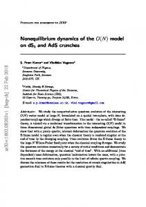
drawn from a zero-mean Gaussian and uniform distributions with varying strengths η0. The parameter η0 is proportional to the standard deviations of the respective distributions so that also their second central moments match. We perform Monte Carlo simulations of the RFIM on a square lattice of the size 256 × 256 at a reduced temperature kBT/|J| = 0.5. We employ the Metropolis dynamics and apply periodic boundary conditions to eliminate boundary effects. In most similar studies, domain (cluster of spins in the same state) sizes were estimated indirectly from the fluctuations in magnetization. In the present study, for better precision we directly measure them by Hoshen-Kopelman algorithm [4]. In order to improve the accuracy and the quality of the results we have performed 50 independent simulation runs, and the resulting quantities presented below represent the obtained average values. 3. Results and discussion The time (Monte Carlo sweep) evolution of the magnetization curves for the RFIM with both uniform (URF) and Gaussian (GRF) random fields of different strengths η0 show similar behavior and thus in Fig. 1(a) we only present the results for GRF. Apparently, the character of the evolution of the magnetization strongly depends on 1 0.7 0.5
η0 = 0.2 η = 0.3 0
η = 0.4 0
0
2. Model and method
M(η , t)
0.3 0.2
The Hamiltonian of the 2D RFIM can be written in the
η = 0.6 0
η0 = 1.0 η0 = 1.4
0,1
η = 1.8 0
η = 2.2 0
0.05
η = 2.6 0
form
H = − J ∑ si s j + ∑ηi si , i, j
(1)
i
where J is the coupling constant, conventionally set to unity, si = ±1 and ηi represent respectively the Ising spin and the quenched random field on the ith site, and denotes the summation over nearest neighbors. In the present study, ηi is *corresponding author; e-mail:
[email protected]
0,01 0
10
1
10
2
3
10
10
4
10
t
Fig.1. Log-log plots of the magnetization time evolution for GRF with the strengths from η0 = 0.2 (top) to η0 = 2.6 (bottom). The dashed lines represent the best linear fits.
Template for Calculation of Length of Manuscript… 0.5
0.07 URF GRF
0.4
0.05
−c η
0
β (η )
β
−c η
µ(η ) = a + b e 0 µ µ URF: c = 1.816 µ GRF: c = 1.852
0
µ (η0)
β(η ) = a + b e 0 β β URF: c = 1.310 β GRF: c = 1.285
0.3
URF GRF
0.06
β
0.2
0.04
µ
0
µ
0.03 0.02
0.1
0.01
0 0
0.5
1
1.5 η
2
2.5
3
0
the strength of the disorder. Namely, before the saturation value is reached the magnetization growth can be characterized by the power law behavior with the η0dependent exponent β(η0). The dependence of the power law exponent β(η0) on the disorder strength η0 is shown in Fig. 2. In both URF and GRF it is found to follow the exponential law with similar decay exponents cβ, given in Fig. 2. Such a decrease of the exponent β with η0 could be expected. With the increasing strength of disorder η0 spin flips are gradually suppressed owing to the presence of the pinning interaction term (the second term in the Hamiltonian) and consequently the domain walls get pinned, leaving the system in a disordered phase. The fact that the URF and GRF exponents take similar values can be ascribed to the universality phenomenon, which assumes the RFIM properties independent on the choice of the RF distribution. In Fig.3 we demonstrate the growth dynamics of the largest domain in the GRF case, again for various values of the strength parameter η0. For weak disorder (η0 ≤ 0.3) we observe three distinct time regimes. The early and intermediate time regimes follow the power law behavior with generally different exponents µ(η0) and ν(η0), respectively, and the late time regime corresponds to the steady state. For larger disorder strengths (η0 > 0.3) there is only one power law regime with the exponent µ(η0). 1 η0 = 0.2 η0 = 0.3 η0 = 0.4 η0 = 0.6 η0 = 1.0
0.7
1
1.5 η
2
2.5
η0 = 1.8
0.6
The variations of µ(η0) with η0 are plotted in Fig. 4 for both URF and GRF. It is evident that, similar to the magnetization behavior, they fall off exponentially, however, the decay exponents cµ are considerably different from the magnetization decay exponents cβ. Nevertheless, the difference between the URF and GRF values is again very small. 4. Conclusions We studied the nonequilibrium behavior of the 2D RFIM with uniform and Gaussian RF distributions. The dynamic evolution of the magnetization exhibited a powerlaw growth with the exponent β(η0), falling off exponentially with the RF strength η0. The growth of the largest domain followed the power law with different exponent µ(η0), which fell off with η0 even faster than β(η0). For weak disorder we observed different regimes at early and later times. No significant differences were found between the uniform and Gaussian RF distributions, presumably due to the universality phenomenon. Acknowledgement This work was supported by the Scientific Grant Agency of Ministry of Education of Slovak Republic (Grant No. 1/0234/12). The authors acknowledge the financial support by the ERDF EU (European Union European Regional Development Fund) grant provided under the contract No. ITMS26220120047 (activity 3.2.). References
η0 = 2.2 η0 = 2.6
0.5
0.4
1
10
2
3
10
3
Fig.4. Variations of the largest domain growth exponent µ(η0) with the RF strength η0 for URF and GRF. The dashed lines denote the best exponential fits to the data points.
η0 = 1.4
0
Λ(η ,t)
0.8
0.5
0
Fig.2. Variations of the magnetization growth exponent β(η0) with the RF strength η0 for URF and GRF. The dashed lines denote the best exponential fits to the data points.
0.9
0 0
10
4
10
t
Fig.3. Log-log plots of the largest domain size as a function of time for η0 = 0.2 (top) up to η0 = 2.6 (bottom). The dashed lines represent the best linear fits to the data points.
[1] Y. Imry, S.K. Ma, Phys. Rev. Lett. 35, 1399 (1975). DOI: 10.1103/PhysRevLett.35.1399 [2] M. Aizenman, J. Wehr, Phys. Rev. Lett. 62, 2503 (1989). DOI: 10.1103/PhysRevLett.62.2503 [3] S. Sinha, P.K. Mandal, Phys. Rev. E 87, 022121 (2013). DOI: 10.1103/PhysRevE.87.022121 [4] H. Hoshen, R. Kopelman, Phys. Rev. B 14, 3438 (1976). DOI: 10.1103/PhysRevB.14.3438