Ð¥. дм ³µ may be computed at a cost comparable to that of symbolic model checking. ..... by preventing the user from âbarking up the wrong tree.â 5.4 Shallow ...
18.3
Dos and Don’ts of CTL State Coverage Estimation Nikhil Jayakumar
Mitra Purandare
Fabio Somenzi
University of Colorado at Boulder
Abstract
In this paper, on the other hand, we are concerned with an assessment of the coverage model based on unreliable observations. We show in Section 3 that the accuracy of the algorithm of [7] can be improved, and we show through case studies discussed in Section 5, that this leads to increased effectiveness of coverage estimation. As explained in Section 4, the improved algorithm is efficient. We identify several issues that are important to make proper use of coverage estimation. We offer the conclusion that coverage estimation requires disciplined use, but can be of great help in the development of comprehensive sets of properties.
Coverage estimation for model checking quantifies the completeness of a set of properties. We present an improved version of the algorithm of Hoskote et al. [7] that applies to a larger subset of CTL; we prove properties of the algorithm and apply it to three case studies. From these case studies we derive recommendations for an effective use of coverage estimation. Categories and Subject Descriptors B.6.3 [Logic design]: Design aids—Verification General Terms: Verification, Algorithms Keywords: Model checking, state coverage, vacuity detection
1.
2. Preliminaries
�� �� � � ���
A Kripke structure � � consists of a finite set ¼ � � , a set of of states , a complete transition relation initial states ¼ � , a set of atomic propositions , and a labeling � . Any atomic proposition in is a CTL function formula, and if and are CTL formulae, then so are: � , � , � , � ( holds at the next time instant), � ( holds until holds), and � ( holds henceforth). The set of states of satisfying formula is denoted by � and is defined inductively on the structure of the formula [5]. Structure is a model for , written , if ¼ � � . When no instead of ambiguity arises, we write �. An ACTL formula is a CTL formula in which negation is restricted to atomic propositions. An ECTL formula is the negation of an ACTL formula. Further common operators are defined as ab� � , �� � � � , �� breviations, e.g., � � ���� � � , and � � � � �� � � �� . Let
be a state,
an atomic proposition, and a �� �, with CTL formula such that . Let �� � ¼ �� � for � , � � if
, and �� � � otherwise. We say that is covered by for if �� � . Let � . We denote by �� the set of �. Then, states in that are covered by for in � � ¼ designates the set of states of covered by for ; it � can be computed, in principle, by model checking experiments for an arbitrary CTL formula . This approach is not practical. Hoskote et al. [7] showed how an approximation of �� ¼ may be computed at a cost comparable to that of symbolic model checking. Their approach involves approximation in two respects. and into and On the one hand, it implicitly transforms ¼ in such a way that iff and �� ¼ ¼ � � ¼ . The purpose of the so-called observability transforma� tion is to boost the coverage of eventuality properties, and simplify the computation. The transformation is implicit in the sense that ¼ the algorithm of [7] works on and , but returns �� ¼ ¼ ; � if � is the function computed by the algorithm of [7], � �¼ ¼ . When the context identifies then � � and , we write . The second approximation comes from the restriction of the algorithm to a subset of ACTL that excludes the disjunction of formulae containing temporal operators. Though �¼ ¼ is computed exactly for formulae in the allowed sub�¼
� � � ��� � � � � � �� � ��
Introduction
Model checking [5] proves whether a system satisfies a set of properties, but does not directly answer the question of whether the properties are adequate to specify its intended behavior. Two techniques have been proposed to address the completeness of the specification: vacuity detection [1, 9], and coverage estimation [7, 8, 4, 3]. While vacuity detection is concerned with improving individual formulae, coverage estimation addresses the question of whether enough properties have been specified. Two main approaches have been taken to establish the comprehensiveness of a set of properties. Katz et al. [8] suggested that the reduced tableau of a set of ACTL properties should be bisimilar to the implementation. Hoskote et al. [7], on the other hand, consider the effect of perturbations of the model checking experiment on its outcome. A perturbation is covered if it causes a reversal in the verdict of the model checker. More precisely, a perturbation is for Hoskote et al. the flipping of an atomic proposition (an observable signal) when the model is in a particular state. If this perturbation causes a property that holds in the original model to fail, then the state is said to be covered for the flipped signal. The perturbations do not affect at all the transitions of the model; they only make the readings of the labels of its states unreliable. This restriction, and a few others, allowed Hoskote et al. to formulate a symbolic algorithm for coverage estimation whose performance is practically comparable to that of a conventional model checker. Their seminal work, however, left several questions unanswered. Chockler and her co-authors [4, 3] have proposed algorithms of greater generality and have extended the coverage approach to linear time specifications. The practicality of their techniques, however, has not been fully established yet.
�
� ��
�
� � � � �� � � �� � � �� � � � �� � ��
� � � � � � � � � � � � �� �� �� � � � � � �� �� � � �� � � � � �� � � � ��� ���� ���� � ��� ���� � � � � � �� � ����� � � ��������� � �� � �� � � � � �� � �� �
� �� � ��
This work was supported in part by SRC contract 2002-TJ-920 and NSF grant CCR-99-71195.
�
����� ����� � ��� � � �����
Permission to make digital or hard copies of all or part of this work for personal or classroom use is granted without fee provided that copies are not made or distributed for profit or commercial advantage and that copies bear this notice and the full citation on the first page. To copy otherwise, to republish, to post on servers or to redistribute to lists, requires prior specific permission and/or a fee. DAC 2003, June 2–6, 2003, Anaheim, California, USA. Copyright 2003 ACM 1-58113-688-9/03/0006 ...$5.00.
� �� �� �
292
�
�
�
� �� � � �
� �� � � �
100
0
90
1 �
Figure 1: Kripke structure for which ��� ¼
¼
Average Coverage(%) Our Implementation
�
��¼ � � � � ��� ��¼ � ��.
set, no covered states are computed for the others. Hence, the coverage of a set of formulae may be underestimated by the algorithm. Let stand for a propositional formula, for a non-propositional ACTL formula, and and stand for arbitrary ACTL formulae. The algorithm of [7] is defined as follows.
�
�
�
��� � � � � � � ��� � � � �� � � � � � � � ��� � �� ��� �� ���� ��� � �� ���� �� ���� ��� � � �� ���� ��� �� ��� �� � ��� �������� ���� � �� ����� � ����� � The functions �� �� � and ��� �� � compute the states reachable from states in � in one step or in any number of steps, respectively.
�
�
if does not appear in if � is propositional, otherwise.
� ��
� ��
�
� �
�
�� , else
�
50
60
70
80
90
100
�
�
40
The covering estimation algorithm of Section 3 takes as inputs a model , a list of properties, and a list of atomic propositions. A naive implementation of the algorithm consists of two nested loops over the elements of the two lists. This wastes time, because the same computation may be repeated. In [7] it was observed that results can be cached. We now show how the memory requirements of the result cache can be substantially reduced. Coverage estimation of a given formula for two atomic propositions only differs in the evaluations of � ; those of �� , ��� , and �� , which take most of the time, can be done once. Hence, our implementation is passed a set of initial states , a CTL formula , and a list of atomic propositions . If is propositional, for all , and returns a list of results; it computes � � otherwise, the algorithm passes to its recursive invocations, and then computes a list of results based on the list(s) returned to it. The list-based approach examines each property once, regardless of the number of observed variables in it. It localizes the uses of results that may otherwise be evicted from a lossy cache, or unduly increase memory requirements. A subformula is examined more than once only if it has multiple instances. Therefore, one can cache only subformulae with multiple instances. In practice, in our implementation, coverage estimation is about as fast as model checking even without caching. An exception is made for the value of ��� ¼ which is required by most formulae. Figure 3 compares CPU times for the improved estimation algorithm and for plain model checking. All experiments were run
Returning to the example of Figure 1, the improved estimation re� � and � � � . turns the exact result for However, for � � � , State 0 is still inaccurately omitted from the covered states. For existential properties we rely on the identities � � � �� �� , from which we � � �� � � and �� derive coverage estimates:
�
30
4. Implementation
����½ � �¾ � �� � � ��½ � � �¾ � �½ � �� � � ��¾ � � �½ � �¾ �
��� �� �� � � ���� � �� � � ��� �
20
�
�� ��� �� � � �� � � � �
where
20
�
30
, and such that flipping the observed atomic proposition at them would cause to fail. This amounts to the search of a match in a bipartite graph for which symbolic algorithm exist [6], but are in practice restricted to small models. For this reason, we choose the trivial lower bound to for �� properties. Figure 2 compares the improved algorithm to the original one for 158 models from [10]. Each model could be analyzed in less than 30 minutes. The plot shows the arithmetic mean of the coverages of all signals appearing in the properties distributed with the models, before any properties were added to increase coverage. The graph shows that there are many cases in which the improved algorithm provides better estimates than the original one. All points below the diagonal are due to overestimates by the original algorithm.
Improving Coverage Accuracy
40
Figure 2: Scatter plot of the initial coverage for the improved and original estimation algorithms. Ten models have 0 coverage for both methods, and 13 have 100% coverage.
As mentioned in Section 2, the algorithm of [7] will sometimes declare a state covered in for signal even if it is covered only for signal . A simple example is shown in Figure 1. For in atomic proposition and � � ,
�, ¼
�. On the other hand, for � � � , though ¼ State 0 should be covered, but �. Notice that passes ¼ vacuously in the structure of Figure 1. The accuracy of coverage estimation is improved by adopting the following definition.
��� � ��
50
Average Coverage(%) Hoskote et al
��
60
10
� � � � � � � � � � ��� ������� � � ��� ��� �� �� �� �� �� ����� �� � � �� � � �� ��� �� � � ��� �� �� � where � � � � �� � � ��� . The initial call has the initial states �¼ and a passing formula as arguments. The algorithm maintains the invariant that at each recursive call �����, � � � �� . 3.
70
10
The remaining functions are defined as follows.
�
80
�
� �
��� � � � �� ��� � � �� � �� � � � ��� ��� �� �� ��� �� � where we have conservatively taken ��� �� �� �� �. Computing a non-trivial lower bound to ���� �� �� would require finding those states that are the sole successors of states in � satisfying
�� �
293
�
���
� �
� �
�
CPU time Our Implementation
100
perfect strategy. The instance we studied uses four piles, each with up to 15 counters, and has 32 binary state variables. A virtue of coverage estimation is that it forces the verification engineer to closely scrutinize the model. This code review led to the realization that a variable of the nim player was redundant. Its elimination improved coverage. Thirteen properties guarantee 100% coverage for the output variables win, lose, turn, for the four piles of counters, and several internal signals. For this model, the original algorithm also reported 100% coverage. Though 13 properties suffice to cover 100% of the states, a total of 36 properties were tested and found to pass. In view of the discussion of Section 5.4, it is recommended that all passing properties developed in an attempt to increase coverage be retained. In particular, one should not thin the set of properties by model checking them in the reverse order in which they were generated, lest the quality of the test set may be adversely affected.
10
1
0.1 0.1
1
10
100
CPU time Plain Model Checking
5.3 The Heap Figure 3: Scatter plot of the CPU times for the improved estimation algorithms and plain model checking. For 19 models, the CPU times do not exceed 0.1 s for both methods.
The third model is of a hardware implementation of a heap data structure that supports the operations PUSH, POP, and TEST. The TEST operation verifies that the key of each element is higher than the key of its parent. The queue is kept in a single read port, single write-port memory. The model is parameterized. We used an instance with four two-bit entries for a total of 24 binary variables. Only the keys are stored, while the data values are abstracted. The list of observed signals contained the primary outputs of the model, as well as internal variables that are used as pointers to the queue memory. Complete coverage was achieved with 84 properties. Their generation required about eight hours of work. Another 30 properties were generated that produced no additional coverage. The original algorithm reports 99.52% coverage. A difference of less than one percentage point may look small. However, two observations are in order. (1) As in the previous cases, the coverage of the original algorithm suffers more from overapproximation. (2) When a few states are left to be covered, incorrect coverage information may be particularly frustrating. In our experience, the user finds it easier to reason in terms of than in terms of its approximation . Therefore, a better approximation of the actual coverage translates in increased productivity by preventing the user from “barking up the wrong tree.”
with VIS 2.0 [2] which we have extended with both the original and improved coverage algorithms. The CPU times were measured on an IBM IntelliStation running Linux with a 1.7 GHz Pentium 4 CPU and 1 GB of RAM. Coverage estimation times include model checking time and account for all signals appearing in all formulae. Most points in the plot fall between the lines and , confirming that the overhead of the estimation algorithm is modest.
� �
5.
� ��
Discussion
In this section, we first present three case studies from the VIS Verification Benchmarks [10], and then draw general observations.
5.1 The Cabbage, Goat, and Wolf Puzzle Our first example is a model of the famous puzzle that asks how a cabbage, a goat, and a wolf can be ferried one at the time across a river. It has four state bits. The algorithm of Section 3 reports that 11 ACTL properties cover all states but two. The two remaining states can be covered by 4 mixed properties. These properties yield no covered states with the original algorithm, which erroneously declares the two states covered by some other properties, but only reaches 94.79% average coverage for all variables. Most of the 15 properties were targeted at particular uncovered states. The following observation helped in finding them. Let be . A a state, and be a propositional formula such that � passing property of the form � � � does not cover for if flipping falsifies . If, in fact, holds, then flipping at only causes a vacuous pass. More useful properties are such that: (1) holds at a predecessor of , and holds at , but fails if is flipped there; (2) � does not hold at , and fails at , but passes if is flipped there. In the latter case, one can also replace � with ��: for the two hard-to-cover states of the puzzle model, the properties had indeed the form � � �� . The model for the puzzle is symmetric in the cabbage and wolf variables. Though the coverage estimation algorithm does not exploit this fact, the user can save considerable effort by doing so.
�
�
�
�
�
�
�
� � �
�
��
5.4 Shallow Properties
�
�
�
Consider a circuit with two complementary ouptuts and . The property � � � covers all reachable states for both and . In general, let invariant � � � be linear in if each � is a propositional formula, and � � ��¼ � � ��½ .
�
�
� �
�
� ��
�� � ��
�
�� �
� �
� �� ��¼ � ��
�
��
�
be a Kripke structure, and let Theorem 1 Let be an invariant linear in such that . Then � ¼ . ��� ¼ �
� � �
The invariant � � � is linear in both and , and every invariant of the form � � � � � � � � is linear in each � . Hence, every property asserting that a signal can be expressed as a combinational function of other signals gives 100% coverage for . The high coverage provided by linear invariants is not necessarily a cause of concern. Consider a model used to check the equivalence of two (deterministic) circuits with outputs ½ � and ½ � , respectively. The property that ensures correctness is � � � � � , which is linear in all its arguments. Though this property does not fully characterize the model, it captures its intent—proving equivalence. Hence, 100% coverage is justified. However, in the nim player of Section 5.2, the variable that holds the position’s value is the exclusive OR of the numbers of counters
��
� �� � � � � � �
5.2 The Nim Player The second model that we have analyzed is a nim player. Two players take turns in removing counters from piles. Each move consists of removing at least one counter from one pile. The model keeps track of the game position and plays one of the two sides with
294
�� �
��� ��
obtained for the unmodified circuit, 6 failed; coverage went from 100% to 99.66%. The six failing properties were easily modified so as to pass on the modified design. This raised coverage to 99.79%. The second optimization allowed two read accesses to the queue memory per clock cycle. This caused three properties to become inapplicable (they referred to a suppressed state), and one property to fail. The failing property was easily fixed. The resulting coverage was 99.33%. In both cases the decreases in coverage were limited, indicating a certain robustness in the face of design changes. Abstraction is important when improving coverage, because the model checker must be run many times. With manual abstractions, there is no guarantee of property preservation when going from the abstract to the concrete system. To test the effects of concretization, we have increased the size of the heap to eight 3-bit slots. A large fraction of the properties required small changes to apply to the new model. After the trivial fixes, seven properties still failed; 4 were added. Coverage for the 81 that passed was 94.97%.
2
1
0
�
�
Figure 4: Kripke structure illustrating the effects of overapproximation on the connection between coverage and vacuity detection. in each pile. A property that asserts that this is indeed the case yields complete coverage of the variables involved, but does little for the verification of the number of counters in each pile. We say that a property is shallow if it specifies a combinational relationship among signals that are not all primary inputs and outputs to the model. To avoid the false sense of security produced by shallow properties, one could restrict the signals in each property to one primary output and an arbitrary number of primary inputs. However, this may be too restrictive when the relationship between inputs and outputs is complex. In such cases, the use of internal signals in properties may afford a decomposition of the covering task, provided the internal signals are adequately, independently verified. This requires discipline in the use of coverage estimation. In contrast to the high coverage of linear invariants, eventuality properties usually contribute little to coverage. For the nim player, the property that states that from a winning position the second player always wins covers only a handful of states. It is disappointing that a property that asserts something both deep (in space) and global (in time) about the model should have such low coverage. However, in our experience, the bulk of coverage is provided by invariants and � properties, which, by contrast, tend to be shallow and local. An effort should be made to include as many deep properties as possible, to balance the bias of the coverage estimation algorithm in favor of the shallow ones.
6. Conclusions We have discussed extensions and applications of Hoskote’s symbolic algorithm for state coverage estimation in CTL model checking. We have argued that the improved accuracy increases the effectiveness of the property generation process. It is our experience that coverage estimation helps one discover properties of the model being verified—sometimes subtle ones. In our case studies we did not uncover any bugs in the models, but we did find one in the model checker. We also identified one redundancy in the nim player. It is important to understand the limitations of the technique to use it effectively. In particular, we have discussed the problems that arise in connection with shallow properties, we have shown what kind of properties can be used to target specific states, and we have explained the relationship between coverage estimation and vacuity detection. We have occasionally encountered uncoverable states; more frequent were the cases in which a few states required ad hoc properties. Achieving high coverage is labor-intensive; a lot can be done in the interface to facilitate the task beyond what is supported by our prototype. For instance, for large models, it is important to have an incremental tool that does not force one to evaluate a formula multiple times. It is also useful to be able to present uncovered states in bundles instead of individually.
5.5 Coverage and Vacuity
�
A CTL formula passes vacuously in model if there is a subformula of that can be replaced by an arbitrary formula without affecting the result of model checking the resulting [1]. If passes vacuously, it can be “vacuum cleaned” [9] by replacing with either ���� or � �. If , the result of the substitution is a stronger formula that still passes in . Hence, it is a more stringent specification of . Vacuity detection and coverage estimation are complementary techniques. The former is concerned with improving individual properties, while the latter is concerned with augmenting a set of properties so that, collectively, they represent a better specification. The following result establishes a link between the two techniques.
� �
�
�
�
�
�
�
References [1] I. Beer et al.. Efficient detection of vacuity in ACTL formulas. CAV’97, pages 279–290. July 1997. LNCS 1254. [2] R. K. Brayton et al.. VIS: A system for verification and synthesis. CAV’96, pages 428–432. July 1996. LNCS 1102. [3] H. Chockler et al.. A practical approach to coverage in model checking. CAV’01, pages 66–78. July 2001. LNCS 2102. [4] H. Chockler, O. Kupferman, and M. Y. Vardi. Coverage metrics for temporal logic model checking. TACAS’01, pages 528–542. April 2001. LNCS 2031. [5] E. M. Clarke, O. Grumberg, and D. A. Peled. Model Checking. MIT Press, Cambridge, MA, 1999. [6] G. D. Hachtel and F. Somenzi. A symbolic algorithm for maximum flow in 0-1 networks. Formal Methods in Systems Design, 10(2/3):207–219, 1997. [7] Y. Hoskote, T. Kam, P.-H. Ho, and X. Zhao. Coverage estimation for symbolic model checking. DAC’99, pages 300–305. June 1999. [8] S. Katz, O. Grumberg, and D. Geist. “Have I written enough properties?” — A method of comparison between specification and implementation. CHARME’99, pages 280–297. Sept. 1999. LNCS 1703. [9] M. Purandare and F. Somenzi. Vacuum cleaning CTL formulae. CAV’02, pages 485–499. July 2002. LNCS 2404. [10] VIS verification benchmarks. URL: http://vlsi.colorado.edu/ vis.
Theorem 2 Suppose is a vacuously passing formula, and that is obtained from it by vacuum cleaning. Then �� ¼ � � ¼ for every and . �
�
� �� � � �
� �� ���
� � � � � ��
Figure 4 shows that it is not possible to replace with in Theorem 2: � passes vacuously because also passes; � � � � �
�, while � �. however, � � �. Notice that � � � In spite of the exceptions, it is usually advantageous to intertwine vacuity detection and coverage estimation. In our study of the heap model of Section 5.3, we noticed that in the majority of cases, vacuum cleaning properties before estimating their coverage resulted in better coverage and less work.
�� � � � � �� �� � � � � �� ��
5.6 Reusability of Properties We considered two optimized versions of the heap model of Section 5.3. In the first, the number of clock cycles required to push an item onto the queue is reduced by one. Of the 84 properties
295