Double Continuum Limit of Deep Neural Networks - Principled ...

Double Continuum Limit of Deep Neural Networks

Sho Sonoda * 1 Noboru Murata 1 and φt : Rm → Rm (t ∈ [0, T ]) is a continuous analog of φ` ’s. In the following subsections, we identify φt as a transport map with depth as time variable t. We then obtain a finite deep neural network as a broken line approximation of trajectory t 7→ φt (x).

Abstract The continuum limit is an effective method for modeling complex discrete structures such as deep neural networks to facilitate their interpretability. The continuum limits of deep networks are investigated with respect to two directions: width and depth. The width continuum limit is a limit of the linear combination of functions, or a continuous model of the shallow structure. We can understand that what shallow networks do is the ridgelet expansion of their approximating functions. The depth continuum limit is a limit of the composition of functions, or a continuous model of the deep structure. We can understand that what deep networks do is to transport mass to decrease a certain potential functional F of the data distribution. A discretization method can potentially replace the backpropagation. Specifically, we can synthesize a deep neural network from broken line approximation and numerical integration of a double continuum model, without backpropagation. In this study-in-progress, we have developed the ridgelet transform for potential field, and synthesized an autoencoder without backpropagation. In this paper, we review recent developments of the width and depth continuum limits, introduce our results, and present future challenges.

The dynamical system viewpoint is not new to recurrent neural networks (Seung, 1998). These days, distributionbased formulations of deep neural networks are successful. For example, they are generative density estimators (Bengio et al., 2013), variational autoencoder (Kingma & Welling, 2014), reverse diffusion process (Sohl-Dickstein et al., 2015) and adversarial generative networks (Goodfellow et al., 2014). In shrinkage statistics, the expression of “transport map” x + f (x) is known as Brown’s representation of posterior (George et al., 2006). Liu & Wang (2016) analyzed it from a Bayesian viewpoint, apart from deep learning, and proposed kernel Stein discrepancy. Recently, we have observed that some kinds of convolutional networks can also be regarded as transport maps. Specifically, the skip connection structure x+f (x) used in highway networks (Srivastava et al., 2015) and ResNet (He et al., 2016) is formally understood as a transport map. 1.1. Wasserstein Gradient Flow of Deep Network Consider a transport map defined by a velocity vector field ∂t φt (x) = ∇Vt (φt (x)),

The continuum limit with respect to depth is a recently developed technique. It is a continuum analogy of the deep neural network, formulated as a formal limit of the composition of functions as below: (1)

where φ` : H` → H`+1 (` = 1, . . . , L) with feature vector space H` is a feature map defined by the `-th hidden layer, *

(2)

with time-dependent potential function Vt : Rm → R, where ∇ denotes the gradient operator on Rm . When t is small, it has an “explicit” expression

1. Depth Continuum Limit

φL ◦ · · · ◦ φ1 (x) → φt=T (x),

x ∈ Rm

1

Equal contribution Waseda University, Tokyo, Japan. Correspondence to: Sho Sonoda . Presented at the ICML 2017 Workshop on Principled Approaches to Deep Learning, Sydney, Australia, 2017. Copyright 2017 by the author(s).

φt (x) = x + t∇Vt (x) + o(t2 ) as t → 0.

(3)

Generally, (2) is rewritten as an integral equation Z t φt (x) = x + ∇Vs (φs (x))ds, 0

however the explicit solution is rarely tractable. An important example of (2) is the Gaussian denoising autoencoder (DAE), where Alain & Bengio (2014) determined that φt (x) = x + t∇ log µt (x) + o(t2 ) as t → 0 with data distribution µt . See Sonoda & Murata (2016) for transport theoretic reformulation of the DAE.

Double Continuum Limit of Deep Neural Networks

Associated with a transport map, we consider data distributions. We write by µ0 the initial state of the data distribution, or the probability density function of the input data x; and by µt its pushforward φt] µ0 , or the probability density function of the “feature vector” φt (x). That is, x ∼ µ0 and

1.2. Example: Gaussian DAE Sonoda & Murata (2016) determined that data distribution µt of the Gaussian DAE evolves according to the backward heat equation ∂t µt (x) = −4µt (x),

φt (x) ∼ µt (:= φt] µ0 .) Recall that a mass transportation is a change of variables, thus the pushforward measure µt satisfies the following equation µt (φt (x)) |∇φt (x)| = µ0 (x),

t ≤ 0, x ∈ Rm .

∂t µt (x) = −∇ · [µt (x)∇Vt ( x)],

x ∈ Rm

and concluded that the feature map of the Gaussian DAE is equivalentR to a transport map that decreases the entropy H[µ] := − µ(x) log µ(x)dx of the data distribution:

(4)

As time t evolves, the data distribution µt changes according to the continuity equation (5)

µt=0 = µ0

d µt = −grad H[µt ], dt

µt=0 = µ0 ,

where 4 denotes the Laplacian on Rm . This is immediate because when F = H, then V = − log µt and thus   ∇µt grad H[µt ] = ∇ · [µt ∇ log µt ] = ∇ · µt = 4µt , µt

where ∇· denotes the divergence operator on Rm . The proof is simply to calculate the change of variables formula (4). This result is intuitively reasonable because the term ∇V in (2) corresponds to a flux from the viewpoint of hydrodynamics.

which means (5) reduces to the backward heat equation.

The continuity equation (5) has no explicit solution either, except for some special cases such as heat equation (Vt = − log µt ). According to Otto calculus (Villani, 2009, Ex.15.10), the solution µt coincides with a trajectory of the Wasserstein gradient flow

Similarly, when F is the Renyi entropy Z µα (x) − µ(x) α H [µ] := dx, α−1 Rm

d µt = −grad F[µt ], (6) dt with respect to a potential functional F that satisfies the following equation: Z d F[µt ] = Vt (x)[∂t µt ](x)dx. dt Rm Here grad denotes the gradient operator on L2 -Wasserstein space W2 (Rm ). The L2 -Wasserstein space W2 (Rm ) is a functional manifold, or the family of probability density functions on Rm equipped with an infinite-dimensional Riemannian metric called the L2 -Wasserstein metric. While (6) is an ordinary differential equation on the space W2 (Rm ) of probability density functions, (5) is a partial differential equation on Euclidean space Rm . Hence, we use different time derivad tives dt and ∂t . The Wasserstein gradient flow (6) possesses a distinct advantage that the potential functional F does not depend on time t. In the following subsections, we will see that both the Boltzmann and Renyi entropy are examples of F. The Wasserstein gradient flow facilitate the interpretability of deep neural networks because we can understand a deep network as a transport map φt that transports mass to decrease the quantity F[µt ] of the data distribution.

1.3. Example: Renyi Entropy

then grad Hα [µt ](x) = 4µα t (x) (see (Villani, 2009, Ex.15.6) for the proof) and thus (5) reduces to the backward porous medium equation ∂t µt = −4µα t.

(7)

O PEN Q UESTION Can we relate a potential functional F and an existing training procedure of deep learning? What is the best discretization strategy of a transport map?

2. Width Continuum Limit The continuum limit with respect to width was developed in the 1990s. It is a continuum analogy of the shallow neural network, formulated as a formal limit of the linear combination of functions as below n X

cj σ(aj · x − bj ),

(aj , bj , cj ) ∈ Rm × R × C

j=1

Z →

c(a, b)σ(a · x − b)dλ(a, b),

(8)

Rm ×R

which is also known as the integral representation of a neural network. Here σ : R → C is an activation function, c(a, b) is a continuous analog of cj , and

Double Continuum Limit of Deep Neural Networks

dλ(a, b) is an appropriate measure. Typically, σ is either Gaussian, sigmoidal function or ReLU; and dλ(a, b) is either the Lebesgue measure dadb or a Borel measure |a|−(m−1) dadb. The integral representation theory is introduced by many authors (Poggio & Girosi, 1990; Mhaskar & Micchelli, 1992; Leshno et al., 1993; Barron, 1993; Girosi et al., 1995; Murata, 1996; Cand`es, 1998; Rubin, 1998) to investigate how shallow networks work.; and further developed by Donoho (2002); Le Roux & Bengio (2007); K˚urkov´a (2012); Sonoda & Murata (2017). These studies are conducted from the standpoint of linear algebra. That is, they regard cj and σ(aj · x − bj ) as coefficients and basis functions respectively. Today, we can understand that what shallow networks do is the ridglet expansion of an integrable function f . Note that it refers only to what they can potentially do and not to what they actually do. Linear algebra was appropriate in the age of shallow networks. However, it lacks considerations of depth, and thus it is inadequate to explain why deep networks perform better than shallow networks. The depth continuum limit made a breakthrough by introducing dynamical system viewpoint and going beyond what they actually do. 2.1. Ridgelet Analysis Ridgelet analysis is a well organized framework of the integral representation theory. The ridgelet transform Rρ f (a, b) of an integrable function f ∈ L1 (Rm ) with respect to a Schwartz function ρ : R → C is defined as Z (9) Rρ f (a, b) := C(a, b) f (x)ρ(a · x − b)dx, Rm

for every (a, b) ∈ Rm × R, where C(a, b) is an appropriate normalizing constant. We σ are admissible when the integral R ∞ say that ρ and −m ρ b (ζ)b σ (ζ)|ζ| dζ exists and not zero. Here b· denotes −∞ the Fourier transform. A typical choice of ρ is a derivative of Gaussian function. When ρ and σ are addmissible, then the reconstruction formula Z [Rρ f (a, b)]σ(a · x − b)dλ(a, b) = f (x), (10) Rm ×R

holds for every f ∈ L1 (Rm ). That is, if we plug the ridgelet transform Rρ f (a, b) in place of the coefficient c(a, b) in (8), the integral representation network behaves R as f (x). Because the integral Rm ×R is an idealized limit Pn of a finite sum j=1 , the reconstruction formula represents the universal approximation property of neural networks.

It is intriguing that, in general, there exist infinitely many different ρ’s that are admissible with the same activation function σ (see § 6 of Sonoda & Murata (2017) for example). It means that there are infinitely many different coefficients c(a, b) that results in the same function f (x). The backpropagation implicitly choose ρ without control, probably depending on the initial parameters, network structure and optimization algorithms. 2.2. Discretization Methods A constructive discretization method can potentially replace the backpropagation. That is, by numerically integrating the reconstruction formula with a finite sum: LHS of (10) ≈

n X

cj σ(aj · x − bj ),

(11)

j=1

we can “synthesize” a neural network that approximates f (x) without using backpropagation. The backpropagation results in the so-called black box network in the sense that no one knows how the trained network processes information, because the training result is simply a local minimizer of a loss function that lacks control on the network parameters. In contrast, the discretization method could provide a white box network because the training result converges to a unique limit without any loss of the parameter controllability. The development of a discretization method with theoretical guarantees such as an error bound and a convergence guarantee is our important future work. Today we have many discretization strategies: regular grid (frame) and atomic decomposition (Donoho, 1999), Monte Carlo integration (Sonoda & Murata, 2014), random feature expansion and/or kernel quadrature (Bach, 2017). Probabilistic numerics (Briol et al., 2016) is an emerging field that aims to unify these methods. Mhaskar (1996) estimated the approximation error as O(n−s/m ) with the number n of hidden units, input dimension m, and smoothness parameter (Sobolev order) s. O PEN Q UESTION Can we really replace backpropagation with discretization?

3. Double Continuum Limit The double continuum limit is the width continuum limit of the depth continuum limit. In other words, it reduces to the ridgelet analysis of a transport map: Z Rρ [id + t∇V ](a, b)σ(a · x − b)dλ(a, b) (12) Rm ×R

where id denotes the identity map. Technically, the ridgelet transform is defined for integrable functions. Hence, we

Double Continuum Limit of Deep Neural Networks

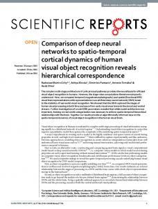
we can obtain an autoencoder without backpropagation. Figure 1 depicts an autoencoder on R2 realized by numerically integrating (15). Note that we omitted calculating the normalizing coefficients and rescaled values instead.

K

●

●

●

●

●

●

●

●

●

●

●

●

●

●

●

●

●

●

●

●

●

●

●

●

●

●

●

●

●

●

2.5

●

●

●

●

●

●

●

●

●

●

●

●

●

●

●

●

●

●

●

●

●

●

●

●

●

●

●

●

●

●

2.0 y

The proof is straitforward as below: Z Rρ [∇V ](a, b) = C(a, b) ∇V (x)ρ(a · x − b)dx K Z = C(a, b) V (x)ρ(a · x − b)n(x)dS ∂K  Z 0 −a V (x)ρ (a · x − b)dx

3.0

(13)

●

●

●

●

●

●

●

●

●

●

●

●

●

●

●

●

●

●

●

●

●

●

●

●

●

●

●

●

●

●

●

●

●

●

●

●

●

●

●

●

●

●

●

●

●

●

●

●

●

●

●

●

●

●

●

●

●

●

●

●

●

●

●

●

●

●

●

●

●

●

●

●

●

●

●

●

●

●

●

●

●

●

●

●

●

●

●

●

●

●

●

●

●

●

●

●

●

●

●

●

●

●

●

●

●

●

●

●

●

●

●

●

●

●

●

●

●

●

●

●

●

●

●

●

●

●

●

●

●

●

●

●

●

●

●

●

●

●

●

●

●

●

●

●

●

●

●

●

●

●

●

●

●

●

●

●

●

●

●

●

●

●

●

●

●

0.0

Rρ [∇V ](a, b) = −a Rρ0 [V ](a, b).

Rm ×R

1.5

We present an integration-by-parts formula for the vector ridgelet transform. Let K ⊂ Rm be a compact set with smooth boundary ∂K. Given that a smooth scalar potential V is supported in K, the ridgelet transform of potential vector field ∇V is calculated by

1.0

3.1. Ridgelet Transform of Potential Vector Field

Therefore, by numerically integrating the integral representation Z (15) −K aρ0 (−b)σ(a · x − b)dadb ≈ idr,0 ,

0.5

consider a transport map with compact support.

0.0

0.5

= 0 − a Rρ0 [V ](a, b).

3.2. Example: Autoencoder As the most fundamental transport map, we consider a smooth “truncated” autoencoder idr,ε . Denote by Bm (z; r) a closed ball in Rm with center z and radius r. We assume that idr,ε is (1) smooth, (2) equal to the identity map id when it is restricted to Bm (r), and (3) truncated to be supported in Bm (r + ε) with a small positive number ε > 0. Let Vr,ε be a smooth function that satisfies  1 2  x ∈ Bm (0; r),  2 |x| Vr,ε (x) := (smooth map) x ∈ B(0; r + ε) \ B(0; r),   0 x∈ / Bm (0; r + ε), and let idr,ε := ∇Vr,ε . Note that we can construct idr,ε and Vr,ε by using mollifiers, and thus such maps exist. The ridgelet transform of the truncated autoencoder is given by Rρ [idr,ε ](a, b) ≈

1.5

2.0

2.5

3.0

x

The LHS of (13) denotes a vector ridgelet transform defined by element-wise mapping, whereas the RHS consists of a scalar ridgelet transform. We can understand the RHS given that the network shares common knowledge among element-wise tasks.

−KC(a, b)aρ0 (−b)

1.0

as

ε → 0 (14)

with a certain constant K. See supplementary for the proof.

Figure 1. Autoencoder on R2 realized by discretizing the ridgelet transform of the truncated identity map, without backpropagation.

O PEN Q UESTION According to Mhaskar (1996), the approximation error is estimated by the Sobolev order s of the transport map id + t∇V . Can we determine any trade-off relation between the smoothness s and depth t? Can we estimate the generalization error?

4. Conclusion We have provided an overview of depth (1) and width (8) continuum limits of neural networks, and developed the double continuum limit (12). We have introduced the ridgelet transform (13) for potential vector fields, and synthesized an autoencoder (15) without backpropagation. As suggested in the Wasserstein gradient flow (6), we expect that what a deep neural network does corresponds to a ridgelet transform Rρ [id + t∇V ] of a transport map id + t∇V that decreases a functional F[µt ] of the data distribution µt . With respect to the double continuum limit, the development of discretization algorithms in collaboration with probabilistic numerics, estimation of the generalization error, are important topics for our future research.

Acknowledgements The authors would like to thank the anonymous reviewers for their helpful and constructive comments. This work is supported by the Waseda University Grant for Special Research Projects Number 2017S-119.

Double Continuum Limit of Deep Neural Networks

References Alain, Guillaume and Bengio, Yoshua. What Regularized Auto-Encoders Learn from the Data Generating Distribution. JMLR, 15:3743–3773, 2014. Bach, Francis. On the Equivalence between Kernel Quadrature Rules and Random Feature Expansions. JMLR, 18:1–38, 2017. Barron, Andrew R. Universal approximation bounds for superpositions of a sigmoidal function. IEEE Transactions on Information Theory, 39(3):930–945, 1993. Bengio, Yoshua, Yao, Li, Alain, Guillaume, and Vincent, Pascal. Generalized denoising auto-encoders as generative models. In NIPS2013, pp. 899–907, 2013. Briol, Franc¸ois-Xavier, Oates, Chris. J., Girolami, Mark, Osborne, Michael A., and Sejdinovic, Dino. Probabilistic Integration: A Role for Statisticians in Numerical Analysis? 2016. Cand`es, Emmanuel Jean. Ridgelets: theory and applications. PhD thesis, Standford University, 1998. Donoho, David L. Emerging applications of geometric multiscale analysis. Proceedings of the ICM, Beijing 2002, I:209–233, 2002. Donoho, David Leigh. Tight frames of k-plane ridgelets and the problem of representing objects that are smooth away from d-dimensional singularities in Rn . Proceedings of the National Academy of Science of the United States of America (PNAS), 96(5):1828–1833, 1999. George, Edward I., Liang, Feng, and Xu, Xinyi. Improved minimax predictive densities under Kullback?Leibler loss. Annals of Statistics, 34(1):78–91, 2006. Girosi, Federico, Jones, Michael, and Poggio, Tomaso. Regularization Theory and Neural Networks Architectures. Neural Computation, 7(1):219–269, 1995. Goodfellow, Ian, Pouget-Abadie, Jean, Mirza, Mehdi, Xu, Bing, Warde-Farley, David, Ozair, Sherjil, Courville, Aaron, and Bengio, Yoshua. Generative Adversarial Nets. In NIPS2014, pp. 2672–2680, 2014. He, Kaiming, Zhang, Xiangyu, Ren, Shaoqing, and Sun, Jian. Deep Residual Learning for Image Recognition. In CVPR, pp. 770–778, 2016. Kingma, Diederik P. and Welling, Max. Auto-Encoding Variational Bayes. In ICLR2014, pp. 1–14, 2014. K˚urkov´a, V˘era. Complexity estimates based on integral transforms induced by computational units. Neural Networks, 33:160–167, 2012.

Le Roux, Nicolas and Bengio, Yoshua. Continuous Neural Networks. In AISTATS2008, pp. 404–411, 2007. Leshno, Moshe, Lin, Vladimir Ya., Pinkus, Allan, and Schocken, Shimon. Multilayer feedforward networks with a nonpolynomial activation function can approximate any function. Neural Networks, 6(6):861–867, 1993. Liu, Qiang and Wang, Dilin. Stein Variational Gradient Descent: A General Purpose Bayesian Inference Algorithm. In NIPS2016, pp. 1–9, 2016. Mhaskar, H. N. Neural Networks for Optimal Approximation of Smooth and Analytic Functions. Neural Computation, 8:164–177, 1996. Mhaskar, H.N and Micchelli, Charles A. Approximation by superposition of sigmoidal and radial basis functions. Advances in Applied Mathematics, 13(3):350– 373, 1992. Murata, Noboru. An integral representation of functions using three-layered betworks and their approximation bounds. Neural Networks, 9(6):947–956, 1996. Poggio, Tomaso and Girosi, Federico. Networks for approximation and learning. Proceedings of the IEEE, 78 (9):1481–1497, 1990. Rubin, Boris. The Calder´on reproducing formula, windowed X-ray transforms, and radon transforms in Lp spaces. Journal of Fourier Analysis and Applications, 4 (2):175–197, 1998. Seung, Sebastian H. Learning continuous attractors in recurrent networks. In NIPS1997, pp. 654–660, 1998. Sohl-Dickstein, Jascha, Weiss, Eric, Maheswaranathan, Niru, and Ganguli, Surya. Deep Unsupervised Learning using Nonequilibrium Thermodynamics. In ICML2015, volume 37, pp. 2256–2265, 2015. Sonoda, Sho and Murata, Noboru. Sampling hidden parameters from oracle distribution. In ICANN2014, pp. 539–546, 2014. Sonoda, Sho and Murata, Noboru. Decoding Stacked Denoising Autoencoders. 2016. Sonoda, Sho and Murata, Noboru. Neural network with unbounded activation functions is universal approximator. Applied and Computational Harmonic Analysis, 43 (2):233–268, 2017. Srivastava, Rupesh Kumar, Greff, Klaus, and Schmidhuber, J¨urgen. Highway Networks. In ICML 2015 Workshop on Deep Learning, 2015. Villani, C´edric. Optimal Transport: Old and New. Springer-Verlag Berlin Heidelberg, 2009.