Mar 16, 1990 - Wyman-Gordon Company, Worcester, MA 01601. 1 ATTN: Technical Library. Lockheed-Georgia Company, 86 South Cobb Drive, Marietta, GA ...
DTWC FILE oMTL TR 90-5
Lf
N1
JAD
STATISTICALLY BASED MATERIAL PROPERTIESA MILITARY HANDBOOK-17 PERSPECTIVE
DONALD M. NEAL and MARK G. VANGEL MECHANICS AND STRUCTURES BRANCH
DTIC S L.ECTE MAR 16 1990U January 1990
S
M
Approved for public release; distribution unlimited.
L.BORATORY COMMAND ~mnmj jupmygy
U.S. ARMY MATERIALS TECHNOLOGY LABORATORY
Watertown, Massachusetts 02172-0001
90 03 15
007
UNCLASSIFIED SECUTTY CLASSIFICATION OF THIS PAGE (Wign DamdEnwmd)
REPORT DOCUMENTATION PAGE . REPORT NUMBER
2. GOVT ACCESSION NO.
BEFORE COMPLETING FORM 3. REC4PIENTS CATALOG NUMBER
MTL TR 90-5 5. TYPE OF REPORT & PERIOD COVERED
Final Report
STATISTICALLY BASED MATERIAL PROPERTIES
A MILITARY HANDBOOK-17 PERSPECTIVE
,. PERFORMING
ORG. REPORT NUMBER
S. CONTRACT OR GRANT NUMBER(s)
7. AUTHOR(s)
Donald M. Neal and Mark G. Vangel 10. PROGRAM ELEMENT. PROJECT, TASK AREA & WORK UNIT NUMBERS
9. PERFORMING ORGANIZATION NAME AND ADDRESS
U.S. Army Materials Technology Laboratory
D/A Project:
Watertown, Massachusetts
AMCMS Code:
02172-0001
P612105.H84
612105.H84XX
SLCMT-MRS 11. CONTROLLING OFFICE NAME AND ADDRESS
12 REPORT DATE
January 1990
U.S. Army Laboratory Command 2800 Powder Mill Road Adelphi, Maryland 20783-1145 14. MONITORING AGENCY NAME & ADDRESS (ifdi&fmentf
13. NUMBER OF PAGES
19 ConJin/ OgCfIc)
15. SECURITY CLASS. (ofdhi'mpon)
Unclassified L.
DECLASSIFICATION/DOWNGRADNG SCHEDULE
16.DISTRIBUTION STATEMENT (ofdtis Rpqort)
Approved for public release; distribution unlimited.
17.DISTR
ON SrATEMENT (e
,abotc ew
in Black 20, iffdffer m Rq~o)
18.SUPPLEMENTARY NOTES
Presented at the Eighth DoD/NASA/FAA Conference on Fibrous Composites in Structural Design, Norfolk, VA 28, November 1989. 19. KEY WOQIRI (Conamua or.
i
if mnemmy and ide,iy
Statistics Material properties Reliability. Design allowables
block nabe,)
Material strength Tolerance limit Composite materials Structural design
20. ABSTRACT (Conasu on o.ww Ade if neemowy and idenab byblock n.mber)
(SEE REVERSE SIDE)
DD
;AN73
1473
E
N
NVUNCLASSIFIED SECURITY CLASSIFICATION OF THIS PAGE ( Whem Data Entued)
UNCLASSIFTED
SECUFIY CUMRCATiON OF THIS PAGE (I*%. Dar Tm..4
ABSTRACT
This report describes statistical procedures and their importance in obtaining composite material property values in designing structures for aircraft and military combat systems. The property value is such that the strength exceeds this value with a prescribed probability with 95% confidence in the assertion. The survival probabilities are the 99th percentile and 90th percentile for the A and B basis values, respectively. The basis values for strain-to-failure measurements are defined in a similar manner. -, The B value is the primary concern of this report.
UNCL ASSIFIED SECURV CLASMFrATION OF THIS PAGE (Wen Dam Emer,/4
CONTENTS
Page INTRODUCTION
............................
1
RELIABILITY ESTIMATES Sample Size - Variability................................................ Definition of the B-Basis Value............................................ STATISTICAL METHODS
-MATERIAL
2 2
PROPERTY VALUES
Flowchart Guidelines...................................4 Goodness-of-Fit Test- Distribution Function.................................. Weibull Method- "B"-Basis Value.......................................... Normal Method- "B"-Basis..............................................
6 7 7
PROCEDURES FOR MULTIPLE BATCHES Anderson-Darling Test.................................................. The Modified Lemon Method............................................. Reliability at Basis Stress Value........................................... Reliability Values - Statistical Versus Deterministic.............................. Effects of Variance on Reliability Estimates...................................
7 8 13 13 14
CONCLUSIONS............................................................
15
ACKNOWLEDGMENTS......................................................
16
INTRODUCTION Many traditional structural materials, which are homogeneous and isotropic, differ from composite materials which have extensive intrinsic statistical variability in many material properties. This variability, particularly important to strength properties, is due not only to inhomogeneity and anisotropy, but also to the basic brittleness of many matrices and most fibers and to the potential for property mismatch between the components. Because of this inherent statistical variability, careful statistical analysis of composite material properties is not only more important but is also more complex than for traditional structures. This report addresses this issue by discussing the methodologies and their sequence of application for obtaining statistical material property values (basis values). A more detailed analysis showing the various operations required for computation of the basis value is presented by the authors in the statistics chapter of the MIL-17 Handbook. 1 The procedures in this handbook required substantial research efforts in order to accommodate various rcquirements (e.g., small samples, batch-to-batch variability, and tolerance limits) for obtaining the basis values. Guidance in selection of the methodology came from the needs of the military, aircraft industry, and the Federal Aviation Administration (FAA). Some of the procedures include determination of outliers, selection of statistical models, tests for batch-to-batch variation, single and multi-batch models for basis value computation, and nonparametric methods. In Figure 1, a flowchart is shown outlining the sequence of operations.
/
BATCH?
\
TEST FOR SIG
FI A T
15NOTHIBATCH-TO-OATCH TET BATC Nto
R
OUTLIERS
ADE S FO R
|)
VARIATION
SA
YES
L
AS
A IO D
TO TH
{ TEST FOR SINIFICANT _
DIR
, _
DIFFERENCE AMONG VAINE
/
1 YES
| SAMPLE FOR SOUTLIERS
INVESTIGATE DEPARTURE FROM STANDARD MODELS AND/O4
SOURCES OF VARIABILITY
WE IBULLNES3
I
W EIBULL
METHOD
NORMAL IT Y
"
METHOD
NORMAL
M ETHOD
Figure 1. Flowchart illustrating computational procedures for statistically-baaed material properties.
1. MIL-IIDBK-17B. Polwne, Matrbr Composites. Naval Publications and Forms Center, 5801 Tabor Avenue, Philadelphia, Pennsylvania 19120, v. 1, February "1998.
An important application of the basis property value is to the design of composite aircraft structures where a design allowable is developed from this value. The process usually involves a reduction in the basis values in order to represent a specific application of the composite material in a structure (for example, a structure with a bolt hole for a particular test and environmental condition). One common approach in the design process requires the design allowable be divided by the maximum applied stress or strain and the result to be greater than one. The basis value is also used in qualifying new composite material systems to be used in the manufacture of aircraft. In this case, the values are obtained from an extensive test matrix, including both loading and environmental conditions. The value also provides guidance in stlecting material systems for specific design requirements. This report also shows how material strength variability and the number of test specimens can affect the determination of reliability numbers. Methods are presented for obtaining protection against this situation by providing a tolerance limit value on a stress corresponding to a high reliability. A comparison between deterministic and statistical reliability estimates demonstrates the inadequacy of the deterministic approach. A case study is presented describing the recommended procedures outlined in the MIL-17 Handbook for determining statisticallybased material property values. REUABIUTY ESTIMATES Sample Size - Variability
The importance of determining a tolerance limit on a percentile value is graphically displayed in Figures 2a and 2b. The cumulative distribution function (CDF) of the standard normal (mean equals 0, standard deviation 1) is plotted for sample sizes of 10 and 50, using 25 randomly selected sets of data. In Figure 2a, for n equals 10, the spread in the percentile is 2.1 for the 10th percentile. In Figure 2b, for n equals 50, the spread is 0.7 for the same percentile. The results show the relative uncertainty associated with small sample sizes when computing reliability values. The range in the percentile can also depend on the amount of variability in the data (i.e., the variance). Often in structural design, a design allowable value is obtained from the basis value. A design allowable is an experimentally determined acceptable stress value for a material (called an allowable stress). The allowable is a function of the material basis value, layup, damage tolerance, open holes, and other factors. It is usually numerically determined for some critical stress region located within the structure. In using the allowable, it is required that the critical stress be less than a proportion (margin of safety) of the allowable stress value. Determining a property value from only 10 strength tests using 90% reliability estimates without confidence in the assertion could result in a nonconservative design situation. In order to prevent this occurrence and provide a guarantee of the reliability value, a tolerance limit (i.e., a lower confidence bound) on the percentile is recommended. The MIL-17 Handbook statistics chapter describes methods for obtaining basis values for a prescribed tolerance limit. Definition of the B-Basis Value
The B-Basis value is a random variable where an observed basis value from a sample (data set) will be less than the 10th percentile of the population with a probability of 0.95. In Figures 3a and 3b, a graphical display is shown of the basis value probability density functions for random samples of n equals 10 and 50, respectively. Samples are from the same
2
population as in Figures 2a and 2b. The vertical dotted lines represent the location of the population 10th percentile (X0 .1 0 ). The probability density functioi of the population is also displayed in the figures. Note that 95% of the time the basis value is less than X0.10 . The graphical display of the basis value density function shows much less dispersion for n equals 50 than for n equals 10; therefore, small sample sizes often result in very conservative estimates of the basis value. 1.A
n=10 Example: Empirical CDF Ix Vn(=p)
p
o o o
1.
-1
.20
4
1
.40
5
1.5
.50
6
1.8
.60
-
2
(a) - -
... ..
Range=2.1
.0 1
1
L
330
7 8
CM0
e.-7
.4
2
==m=/
-7---
1.9 2.1
i.
.70 .80
2.3
1
-1
-
'.
-I
.90
-
a
-
°
0._,= 0 0.3
I.
-.
(b)
... Mean
0
a..
_.__
I
.
I
SD =1 SI
I
62-
~n~ r=
o
I
-_
__ 0-
--
_.
I
Ix
_
__ _ _-__
_
_ __
_ _ _
~ ~Range=. -3
-2
-1
g
X
3
Figure 2. Sample size effect on reliability. Random data sets of size n from a normal distibution.
4
IASISWALUC
PIOCASILITY DENSITY AT X X0
i4
0.-4-
N=10
95%
*
1.4.
(a)
90%
Density a.@-
95,,'/ i qAO11IfT FUNCTION
N=50
DEN(0~STY
95%i "4
e
.0
oaI
Figure 3. Basis value probability density function.
STATISTICAL METHODS
-
MATERIAL PROPERTY VALUES
Flowchart Guidelines
Since the statistical F rocedures and the flowchart (see Figure 1) have been published in the MIL-17 Handbook," this report will only present a brief description of the methods. The purpose, interpretation of results, and the order of application suggested by the flowchart will be the primary objective of this report. The authors have written a computer code which performs the necessary computations for obtaining the basis values as described in the flowchart. The code is available on a diskette, which can be used on various computers, including PCs that are IBM compatible. Both the executable and source code are on the diskette. This code is available free of charge from the authors. The flowchart capability was tested by a 'pplying the recommended procedures using both real and simulated data sets. The results of the simulations showed at least 95% of computed values were less than the known 10% point, this is consistent with the definitions of "B"-basis value, see References 1 and 2. 2. NEAL, D. M, VANGEL, M. G., and TODT, F. Deention of Statistically Based Composite Material Properties in Engineered Materials landbook. Composites, C. A. Dostal, ed., Arican Society of Metal Press, Metals Park Ohio, v. 1, 1987.
4
The flowchart has two directions of operations; one is for the single batch (sample) and the other is for the multi-batch case. A batch could represent specimens made from a manufactured sheet of composite material representing a roll of prepreg material. Published MIL-17 Handbook basis values are usually obtained from five batches of six specimens each. Initially, let us assume the user of the flowchart has only a single batch, or more than one batch but that the batches can be pooled so that a single sample analysis can be applied. The first operation (see Figure 1) is to determine if outliers exist in the data set. A more detailed discussion of outlier detection schemes and applications are published in Reference 3. The method selected is called the Maximum Normed Residual (MNR) procedure 4 and is published in the MIL-17 Handbook. It is simple to apply and performs reasonably well, even though it assumes that the data is from a symmetric distribution. The analysis requires obtaining an ordered array of normed residuals, written as: NRi = (xi - x)/s, i = 1, ---n,
(1)
where i is the mean, s is the standard deviation (SD), and n is the sample size. If the maximum absolute value of NR i (MNR) is less than some critical value (CV), ' 2 then no outliers exist. If MNR is greater than CV, then an outlier X is determined from the largest NR i value. Outlying test results are substantially different from the primary data. For example, assume that the data set contains 16 strength values and 15 range from 150 to 200 ksi, while the other is 80 ksi. The MNR method would identify the 80 ksi value to be an outlier. The 80 ksi specimen should be examined for problems in fabrication and testing. If a rationale is determined for rejecting this test result, then do not include the outlying test value in the data set when obtaining the basis value. If there is no rationale for rejection, the outlier should remain unless the test engineer believes that a nondetectable error exists. It is important to identify the existence of outliers, but it is also of equal importance to resist removing the values unless a rationale has been established. Leaving in, or arbitrary removal of, outlying values can adversely affect the statistical model selection process and, consequently, the basis value computation. An outlier in a data set will usually result in a larger variance and a possible shift in the mean when compared with the same data without the outher. The amount of shift and the variance increase depends on the severity of the outlier (distance removed from the primary data set). It is suggested that for small samples (n is less than 20) critical values corresponding to a 10% significance level be used '2 in order to identify outlying values. If the sample is greater than 20, then use the 5% level. It is often difficult to test for outliers when there is a limited amount of data; therefore, the 10% level will provide additional power to detect outliers. This level will also result in more chance of incorrectly identifying outliers. Outliers can be incorrectly identified from data sets with highly skewed distributions; therefore, it is suggested the box-plot method' "3 be applied for determining outliers in this situation.
3. NEAL, D. M., and SPIRIDIGLIOZZI, L An Efflciou Me"hod for Debamn'ing "A" and "B"Allowabla. ARO 83-2 in Proceedings of the 28th Conference on the Design of Experiments in Army Research, Army Research Office, 1983, p. 199-235. 4. STEFANSKY, W. Rejecting Outkien in Facrial Designs. Technometriz, v. 14, 1972, p. 469479.
5
Goodness-of-Fit Test - Distribution Function Referring to Figure 1, the next step is to identify an acceptable model for representing the data. In the order of preference, the three candidate models are Weibull, normal, and the nonparametric method. The Weibull model is:
Fw(x) = 1 - exp[(x/a) ],
(2)
where x is greater than 0, a is the scale parameter, and fP is the shape parameter. This model is considered first in the ordering of the test procedures. The Anderson-Darling (AD) goodness-of-fit test statistic 1' 5 is suggested for identifying the model because it emphasizes discrepancies in the tail regions between the cumulative distribution function of the data and the cumulative distribution function of the model. This is more desirable than evaluating the distributional assumptions near the mean, since reliability estimates are usually measured in the
tail regions. The Anderson-Darling test statistic and the observed significance levels computations are described in References 1 and 2. Example problems are also shown in Reference 1, demonstrating computational procedures for applying the AD method. In following the flowchart, if the Weibull model hasn't been accepted as a desired model, then a test for the normal distribution is suggested, FN(X) =
1
(2 ) 1/ 2
X fexp[-(t p) 2 /2a 21dt,
(3)
where ju is the mean and a 2 is the variance. The AD tests for the normal model is similar to the test for the Weibull. The procedure used to identify the normal model is also in References I and 2. It should be noted that for small samples reliable identification of a model to represent the data is difficult unless some prior information of the population is known. If the Weibull and normal models are rejected, then a nonparametric method can be used to compute the basis value (see the flowchart). This method does not assume any parametric distribution, as described above. Therefore, model identification is not required, although application of the method can often result in overly conservative estimates for the basis value. The conventional nonparametric method 6 requires a minimum of 29 values in order to obtain a "B"-basis value, and 300 are needed for the "A"-basis number. This report presents a method for obtaining "A" and "B" basis values for any sample size. The method is a modification of the Reference 7 procedure involving the ordered data values arranged from least to largest with the basis value defined as: B = X(r) (X(l) / X(r))
(4)
where X(r) is rIh ordered value and X(I) is the first ordered number. In References I and 2, tables for r and K values are tabulated for sample sizes n. Note, in the case where "A" values are required for small sample sizes, it is suggested that nonparametric methods be applied unless 5. ANDERSON, T. W., and DARLING, D. A A Test of Goodness-of-Fi. J. Am. Statis. Assoc., v. 49, 1954, p. 765-769. 6. CONOVER, W. J. Practical Nonparamctric Statistics. John Wiley and Son$, 1980, p. 111. 7. HANSON, D. L, and KOOPMANS, L H. Tolerance Limits for &6 Clan of Disiduons Wth IncreasingHazard Raws. Annals of Mathematical Statislics, v. 35, 1964, p. 1561-1570.
6
some prior information of available in the lower tail of the reliability numbers. path exists; therefore, it is
the model is known. This is because of the limited information region of the distribution, which can result in erroneous estimates The "A"-basis value is often used in design where a single load essential that the value be conservative.
Weibull Method - B-Basis Value Returning to the sequence of operations, as outlined in the flowchart, if the Weibull model is accepted, then determine the basis value from the following relationship: B =a
[In ( 1/P.)] 1
,
(5)
where fi and a^ are maximum likelihood estimates of the shape f# and scale a of the Weibull distribution. That is, these estimates maximize the likelihood function, which is the product of probability densities for the Weibull model evaluated at each of the n data values. Tables for PB, as a function of the sample size n and the code for determining a and fi, are given in References 2 and 3. Normal Method - "B"-Basis If the Weibull model was rejected and the normal model is an acceptable representation of the data, then compute the basis value as:
B
=
X -
(6)
KBS,
where X and S are the mean and SD, and KB is obtained from tables in References 1 and 2. PROCEDURES FOR MULTIPLE BATCHES Anderson-Darling Test If there are more than one batch of data being analyzed, then a significance test is required in order to determine if the batches may be pooled or if a multi-batch statistical analysis is to be applied (see the flowchart). Note, the outlier test is to be applied to pooled data prior to testing. The recommended test is the K-Sample Anderson-Darling Test 1, which determines if batch-to-batch variability exists among the K batches. This test is simila- to the AD test for identifying acceptable statistical models for representing data. In the K sample case, paired comparisons are made for the empirical CDFs, while the other AD methods compare a parametric CDF with an empirical CDF. In all cases, this comparison involves the integration of the squared difference of the CDFs weighted in the tail region of the distribution. The K-Sample AD is basically a two-sample test in that each sample (i' h batch) is individually compared with the pooled K-1 other batches, repeated K times until each it h batch has been compared. The average of these K two-sample tests determines the K-Sample AD test statistic. Tables of critical values and a detailed description of the method and its application are shown in References 1, 2, and 8. If a significant difference is noted among the K batches, then, as shown in the flowchart, a test for equality of variance is suggested using a method in Reference 9. Application of 8. SCHOLZ, F. W., and STEPHENS, M. A K-Sample Anderson-Daring Tests. 1. Am. Statis. Assoc., v. 82, 1987, p. 918 9. LEHMANN, E L Testing Statistical Hypothesis. John Wiley and Sons, 1959, p. 274-275.
7
the method, tables, and the necessary relationships for computing the test statistic are given in References 1 and 2. The variance test is suggested only as a diagnostic tool. Sample test results that have large variances relative to the other batches may identi[y possible problems in testing or manufacturing of the specimens. Equality of variance is not required when applying the Modified Lemon method, as discussed below, in the multi-batch case. Although the Modified Lemon method is based on the assumptions of equality of variance and normality, simulation results have shown that these assumptions are not necessary. After testing for equality variance, it is suggested that the basis value be obtained from application of the Modified Lemon method (see Figure 1). The Modified Lemon Method Composite materials typically exhibit considerable variability in strength from batch to batch. Because of this variability, one should not indiscriminately pool data across batches and apply single batch procedures. The K-Sample Anderson-Darling Test was introduced into the MIL-17 Handbook in order to prevent the pooling oi data in situations where significant variability exists between batches. For the situation where the K-Sample Anderson-Darling Test indicates that batches should remain distinct, a special basis value procedure has been provided. This method, referred to as the "ANOVA" or "Modified Lemon" method, will be discussed next. A detailed description for applying the method is shown in References 1 and 2. For a discussion of the underlying theory, see Reference 10, the original Lemon paper, and Reference 11, the Mee and Owen paper which modifies the Lemon method. The Modified Lemon method considers each strength measurement to be a sum of three parts. The first part is an unknown constant mean. If one were to produce batches endlessly, breaking specimens from each batch, the average of all of these measurements would approach this unknown constant in the limit of infinitely many batches. Imagine, however,
that one were to test many specimens from a single batch. The average strength approaches a constant in this situation as well, but this constant will not be the same as for the case where each specimen came from a different batch. The average converges to an overall popu-
lation mean (a "grand mean") in the first case, while the average converges to the population The difference between the overall popula-
mean for a particular batch in the second case.
tion mean and the population mean for a particular batch is the second component of a strength measurement. This difference is a random quantity, it will vary from batch to batch in an unsystematic way. We assume that this random variable has a normal distribution with a mean of zero and some unknown variance, which we refer to as the "between batch" com-
ponent of variance. Finally, in order to arrive at the value of a particular strength measurement, we must add to the sum of the con tant overall mean and a random shift, due to the present batch, a third component.
specimen in each batch.
This is another random component which differs for each
It represents variability about the batch mean.
It also is assumed
to have a normal distribution with a mean of zero and an unknown variance, which is referred to as the "within batch" component of variance. The "Modified Lemon" method uses the data from several batches to determine a material basis property value which provides 95% confidence on the appropriate percentile of a randomly chosen observation from a randomly chosen future batch. This basis property 10. LEMON G. H. Factors and One-Sided Tolerance Boundy fr Balanced One-Way ANOVA Random Effects Model. J. Am. Stalis. Assoc., v. 72 1907, p. 676-680. 11. MEE, R. W., and OWEN D B. Improved Facors for One-Sided Tokrance Limits for Balanced One-Way ANOVA Random Effects Model. I. Am. Statis. Assoc., v. 79, 19. p.901-905.
8
provides protection against the possibility of batch-to-batch variaL.lty resulting in future batches which have lower mean strength than those batches for which data are available. To see what this means, imagine that several batches have been tested and that this statistical procedure has been applied to provide a "B"-basis value. Now, imagine that another batch was obtained and a specimen tested from it. After this, still another batch was obtained and a specimen tested from it. If this process were repeated for infinitely many future batches, a distribution of strength measurements corresponding to a randomly chosen measurement from a random batch would be obtained. There would be a 95% certainty that the basis value which was calculated originally is less than the tenth percentile of this hypothetical population of future measurements. This is the primary reason why the Modified Lemon method is advocated by the MIL-17 Handbook, it provides protection against variability between batches which will be made in the future through the use of data which is presently available. An illustrative example of this method applied to nine batches of material is shown below. The data sets did not pass the K-Sample AD Test for pooling. Let the batches be: 1
2
3
4
5
6
7
a
9
61.3
66.5
66.0
61.9
68.9
75.8
72.8
71.9
68.7
68.5
64.7
72.7
68.0
65.0
75.2
75.0
71.0
76.3
62.5
64.9
67.1
63.3
70.9
71.5
66.3
69.5
76.6
66.0
65.2
67.7
74.6
65.4
69.6
69.5
69.5
66.2
66.6
70.3
65.7
66.2
66.5
66.1
71.9
72.6
72.4
64.8
68.2
64.9
74.6
72.8
69.5
69.1
109.6
with a single outlier, 109.6 determined from MNR method. Let's assume 109.6 was an incorrect test result and replaced by 69.6, a corrected test value.
After a substantial amount of computation" 2 involving sums of squares, within batch and between batch variances, noncentral t distribution, etc., the "B"-basis value is: "B" = 60.93.
The summary statistics are shown below. Batch
ni
1
7
65.60
2.99
2
5
66.32
2.33
3
5
67.84
2.84
4
7
67.33
4.17
5
6
66.93
2.45
6
5
71.64
4.03
7
5
71.10
3.33
8
6
71.52
1.98
9
7
71.80
3.88
S1
9
It should be noted, the value of 60.93 is lower than 61.9 of nonparametric solution from the pooled sample. The Modified Lemon method can be overly conservative (low basis values) in order to guarantee 90% reliability with 95% confidence. The number of batches and the variability between and within the batches affect the computation of the basis value. If there are few batches and large between batch variability with small within batch variability, then this situation could result in very low basis numbers, depending on the amount of variability and number of batches. In Figure 4, results from application of flowchart procedures are shown for three batches of five specimens of AS,4/Epoxy material tested in compression. In this case, the mean strength values show a small amount of variability, while there is a relatively large spread within each data set. "B"-basis results from the flowchart application are for the following: ANOVA (Modified Lemon), Weibull, normal, lognormal, and nonparametric methods. A list of assumptions that were violated are not included in the flowchart results. The results show a small difference in basis values, except for the nonparametric solution which has the low value of 167.1. The Weibull method was suggested since it passed the K-Sample AD Test and the AD goodness-of-fit test. The relatively large within batch variances and small differences in mean values made it possible to pool the batches. Batch 1: Mean strength - 221 Ksi Batch 2: Mean strength - 222 Ksi Batch 3: Mean strength - 220 Ksi
200
205
215
210
220
225
230
235
BASIS .VALUE
METHOD
202.8 196.5
.ANOVA Weibil
Normal 199.1 Lognomal 199.6 Nonparametric 167.1 The Weibull result is recommended the Flowchart.
Kai Ksi
Ksi Ksi Ksi by
3 batches of 5, AS4/Epoxy compression)
Figure 4. Example of basis value calculation: Negligible batch-to-batch variability.
Figure 5 shows another result of computing the "B"-basis values using the ANOVA, Weibull, and normal methods applied to another three selected batches from the same population, as shown in Figure 4. The ANOVA result of 15.7 ksi is substantially lower than those from the other two methods. Unfortunately, this is a result of a large difference in mean values preventing pooling of the batches resulting in the required ANOVA application. The large difference in mean values, in addition to relatively small within batch variability, resulted in this extremely low basis value. A "B" value of 6.5 was obtained from the simple normal
analysis using the three mean values.
The result shows that, for this example, the ANOVA
10
method primarily depends on the batch means. The above results would suggest obtaining more batches or investigating testing and processing procedures. Batch 1: Mean strength - 181 Ksi Balch 2: Mean atrength - 236 Ksi Batch 3: Mean alrength - 241 Ksi A "A
160
180
A
200
220
240
260
OASIS VALUE
METHOD
ANOVA
15.7
Kai
Weibull Normal
161.9 159.3
Ksi Ksi
The ANOVA result is recommended by the Flowchart. Normal analysis using only the three mean values gives a Bbasis value of 6.5. Either reject the malerial as too variable or obtain more batches. (3 balches of 5, AS4/Epoxy compression)
Figure 5. Example of basis value calculation: Substantial batch-to-batch variability.
In Figure 6, results are shown for the case of randomly selecting another batch from the same population described in Figure 5. In this case, the ANOVA result shows a value of 105.4 ksi, which is substantially larger than the 15.7 ksi recorded for the three batches. The importance in having a larger number of batches is shown from these results in Figures 5 and 6. Also, with more data available, the pooled results for the Weibull and normal model also resulted in less conservative values. Figure 7 presents results showing where a substantial amount of within batch data is not necessary. In Case 1, the ANOVA results for three batches of 100 data values each, resulted in 154.9 ksi, while for Case 2, three batches of ten each, a "B"-basis value of 152 ksi was obtained. This result emphasizes the importance of being able to obtain more batches rather than increasing the batch size. However, the ANOVA results in Figure 4 show three batches can provide reasonable results similar to pooled results if small differences in mean values relative to batch variances exist. Note that for very large batch sizes, the K-Sample AD Test can reject pooling of data even though there is a small difference in mean values. This rejection is statistically correct, but the user of the flowchart may consider the difference in the batch means not of engineering importance. In this case, the user can make the decisior of pooling or not pooling, since there will be a small difference in basis values from pooled or unpooled results. If there are large batch differences and the ANOVA method is suggested from the flowchart, then adding more batches can reduce the conservatism. The ANOVA method is a random effects model which determines a basis value representing all future values obtained from the same material system and type of test. In order to provide this guarantee in the presence of large batch-to-batch variability, there is the potential for it to be overly conservative, which was shown in Figure 5. 11
1: 2: 3: 4'
Batch Batch Batch Batch
Mean Mean Mean Mean
strength strength strength strength
- 181 Ksi - 236 Ksi - 241 Ksi - 217 Ksi
*
A 160
A
A&A I
180
*4I
I
I
200
220
•
240
-
260
METHOD
BASIS VALUE
ANOVA
105.4 170.3 170.0
Welbull Normal
280
Ksi Ksi Ksi
The ANOVA result is recommended by the Flowchart. A single additional batch increased the basis value from 15.7 Ksi to 105.4 Ksi.
(4 batches of 6, AS4/Epoxy compression)
Figure 6. Example of basis value calculation: The effect of an additional batch.
Case 1: T300/Epoxy Unidirectional Tension 3 batches of 100 specrnens each Basis Value
Method
154.9 171.7 175.7
ANOVA Weibull Normal
Case 2: One random detaset of 10 Irom each of the above three batches. 3asis Value
Method
152.0 165.7 172.5
ANOVA Weibull Normal
The ANOVA method is recommended by ihe Flowchart.
Note
that there is little
diflerence between basis values for batch sizes of 10 and basis values for batch sizes 01 100. Figure 7. The effect of Increased batch size: Subetantial
between batch variability.
12
Reliability at Basis Stress Value
Figure 8 conceptually describes the statistical reliability of a simple structure in tension as it relates to the "B"-basis applied stress value. In the example shown in the figure, ten percent of all the specimens (structures) will fail when subjected to load S. This statement should be incorrect at most one time in twenty (95% confidence). S is the "B"-basis value obtained from strength (failure load) measurements from specimens of the same material and geometry. This statistical guarantee that at most 10% of the specimens will fail, can provide the engineer with a quantitative number for selecting and applying materia! in composite material structures. This is unlike the conventional deterministic property value approach which is an ad hoc procedure that reduces the mean strength measurements in order to obtain some design value which can result in a potentially over or under design situation. In applying the statistical basis value, it is assumed the material, geometry, and loading conditions in the structural design situation is similar to those obtained from the strength measurements. This is also true for deterministic property value applications. In the following sections the inadequacies of the deterministic approach are discussed in more detail.
The reliability ofa
test specimen at the 3-basis stress
should be high. For a statistically based 8- basis value calculated from a procedure appropriate to the data. this reliability Is guaranteed to be at least 20% (i.e., 90% with 965% confidence).
S - B-basis alress
N specimens of which F fallat or below stress S. Estimated reliability at 8-basis stress
(N-F)/N
Figure 8. Reliability at basis stress: Statistical versus deterministic.
Reliability Values
-
Statistical Versus Deterministic
In Figure 9, the results of a simulation process involving the random selection of ten values from a population of 191 strength measurements repeated 2,500 times, are graphically displayed. For each simulation, a design number or material property value is obtained from each of the three procedures X/2, (2/3)X, and the MIL-17 flowchart. The mean value of the data set is X. The reliability values, as shown in the figure, are obtained by evaluating the population probability distribution fit to the 191 values at the design numbers. In the case where the mean is reduced by a factor of 1/2, the strength values are very low (90 ksi) and the reliability is extremely high (1.0). The engineer may not be able to
13
afford such a high reliability value of 1.0 (to twenty significant digits) at the expense of having design values as low as 90 ksi when mean strength is 180 ksi. The factor of 2/3 increases the design value but reduces the reliability to approximately 0.999. The flowchart "B"-basis calculation provides higher strength values with acceptable reliability numbers. The other two procedures show an element of uncertainty by depending on the chosen factor. If the engineer used the factor of 1/2, this would result in an extreme over-design situation requiring either rejection of the material or the design. Alternatively, if the engineer used the mean strength as the design number, the reliability would be reduced to 0.5, although strength values would be much higher. The flowchart procedure removes the uncertainty by providing a guaranteed minimum reliability of 0.90, without unnecessarily reducing the basis value. The minimum reliability can be increased to 0.99, if necessary, by using "A"-basis computations, as outlined in the MIL-17 Handbook.
Population: 191 strength values Detaset: 10 specimens chosen 2500 times randomly
strength s0
100
120
140
(.9gg)
-. 098)
160
10
(1.0)--41.0) i/2 "X/ 1.5
(.97)
(.918) B-ba si(Flowchart)
) Reability Values (T3OO/Epozy Unidirectional)
TENSION
Figure 9. Reliability/strength comparison: A cae study statistical versus deterministic.
-
Effects of Variance on Reliability Estimates In Figure 10, the effects of variance differences, as they relate to reliability estimates, are shown from a simulation process. This involved randomly selecting ten values from each of two separate normal distributions with the same mean of 100 and different SDs of 5 and 25 repeated 2,500 times. The reliability values are obtained in a similar manner, as described in the previous section, except the probability values were obtained from the normal distribution. In the case where the SD is 5, there is very little dispersion in the reliability values. Again, the design number from X/2 is substantially lower than the basis value using the flowchart process, although the reliability is very high for this number. Note that when SD is 25, there is a substantial increase in the dispersion of the reliability values, particularly for the basis value using the flowchart method. The flowchart results show similar reliability estimates for both SDs of 5 and 25, although for the X/2 the reliability has beenreduced substantially from twelve nines to 0.96. This is the result of the deterministic (Xi2) approach being independent of variance. This is not an issue if 50% reliability is required, but for 90% reliability,
14
variability is important. Dividing the mean by two can be nonconservative for a situation when the distribution has a large spread (long tail). In order to made an adjustment for this situation, the flowchart method (basis value) is suggested (see the results in the figure where the basis value adjusts to a lower level but maintains the same range for the reliability estimates). The basis value will guarantee a reliability by adjusting the design value, while the safety factor approach cannot guarantee reliability. This result suggests using the basis method if it is important to maintain a certain level of reliability. The overall issue is that the flowchart methods will provide property values with specified reliability with 95% confidence, while the deterministic approach is an ad hoc approach with no control of the resulting reliability estimates. Population mean 100, 10 values per dataset
Standard
Deviation
strength
... ) (.99)-(.93)
(.999 ... )--.
/1.5
(99~**
I
SE
.0A
f
I
a I1. I
a
sa
.
00 Eo 3t
c0
SO
I
ZDM
-00 2-
0.
e -0
u
I
-II
do
I
]so
CF
.3
E
-OI
CL4
L
0
CI5 I
-3C
.5
II7dt
>
I-
~. c-d I
-1
0 =E0O-I
I
z
w
I
*
0Z W JI
Eo
& 2
c,
_
g
CC2
E CL~8
DC
2 r, a.E
C
C6U
8
z
.cw1
g
0i al
a
Z
Il*
~
a- o
~
~
3
Q
& t*-0.8
E
OSa . L-----------------------------------------------1.---------------------------------------------
IAa