cure is implemented by the following way. A model of CPU architecture is being ... ed performance indices (such as working time, idle time, processor utilization ...
�
DYANA: An Environment for Embedded System Design and Analysis R.L. Smeliansky, A.G. Bakhmurov, A.P. Kapitonova Moscow State University, Dept. of Computational Mathematics and Cybernetics, Vorobyevy Hills, Moscow 119899, Russia, e-mail: smel,bahmurov,alla @cs.msu.su �
Abstract The results presented here are based on many years of experience of development and application of DYANA – an environment for analysis of multiprocessor computer systems operation. The architecture and basic features of such an environments are discussed. Main problems arizing during such an environments design are highlighted and possible solutions are shown. The key features of the DYANA environment are: the possibility of both quantitative and algorithmic analysis of system to be modeled; the time complexity estimation subsystem which helps to avoid the instruction-level simulation of target computer system; support of program development through simulation.
1. Introduction Usually, simulation is a significant stage of a product’s life cycle. More complex the product is, more substantial the simulation stage is in the life cycle. The suitability of simulation modelling from the viewpoint of software development manufacturability depends on answers on two questions: to which extent the transition from the model to the product itself is simple and efficient? �
how manufacturable the process of simulation model creation and investigation is? �
In other words, how the process of model creation and investigation ’fits’ into the process of product development? From the viewpoint of model-to-product transition, it’s perfect when we obtain the product as a result of simulation, or the transition is automated completely. �
This work is partially supported by the Russian Fund of Basic research. Grant No. 98-01-00151 This work is partially supported by the EEC INCO-Copernicus Grant No 977020 �
�
In this article we’ll investigate the model-to-product transition with respect to such an objects as embedded multiprocessor systems. The state-of-the-art technology of developing such a systems is characterized by the following. In the area of hardware, there exist mature technologies for automated transition from hardware description to its implementation. As a rule, this hardware description is a result of simulation. But, the transition mentioned above is developed for the chip level only and implemented in the CAD systems based on the VHDL and Verilog languages. Now the support for such a transition starting from the systems level is ’hottest’. There are many reasons for this, the main one is: the speed of hardware development now is far beyong the one of software development [9]. Authors do not know any design environment enabling the modelto-product transition starting from the systems level. In the area of software development, simulation is not used in practice. Various specification methods does not give the opportunity to estimate the properties of program under development with respect to the particular hardware environment. The manufacturability of simulation model development and investigation strongly depends on the concepts of simulation environment being used, on how this environment covers all development stages. Such an environment should include at least the following: a simulation modelling language, a programming language (if we wish to obtain a program as a product) or a hardware description language (if the product is a hardware component), a system behaviour specification language. Aproppriate graphical facilities, editors, compilers etc. are required as for model as for program development. For the last 30 years, more than 200 languages and environments were proposed [16], with various concepts and capabilities. But, none of them was directed to investigation and development of multiprocessor distributed computer systems. These environments use different languages on different steps (e.g. for model description, for specification etc.). So the problem of syntactical and semantical consistency arizes immediately.
All these environments has different architecture. The absence of stable and unified architecture (which is clear and convenient for user and provides integration of all necessary tools) complicates the problem of portability and working with this environments in theclient-server network architecture. We’ll try to answer the questions mentioned above and show possible solutions on the case of the DYANA system applied to problems of development and analysis of operation of distributed multiprocessor computer systems.
2. Project goals The DYANA system (DYnamic ANAlyzer) is the software system which is proposed to help analyze distributed computer environment operation. The design and development of the system were aimed at the following: to develop the tool for describing as software behaviour as hardware behaviour of distributed systems on the systems level; �
to develop the tool for systems performance estimation under the different tradeoffs between hardware and software on the project system level stage; �
to enable the application of algorithmic and quantitative methods of analysis to the same model description [15]; �
to have a possibility to vary the detail level of behaviour analysis depending on the detail devel of description; (this goal has a ’side effect’: to investigate the methodology of program development through simulation and stepwise refinement); �
to experiment with a simulation models of software and hardware independently. �
The goals mentioned above imply the solution of the following problems: how to describe such particularities of modeled object as indeterminism of program behavior, independence of program behavior from time, absence of unique time in a distributed system, shared resourses, existence of two types of parallelism - interleaving and real concurrency? �
how to measure the ”computational work” of the program being analyzed and how to map the measure onto time for given hardware environment? �
�
how to provide the technology for the development of a model to support the ”top-down” approach, to enable re-usage of model components?
�
how to integrate all tools involved in product development?
In other words, the main goal of the project is to develop an instrumental environment which enables the user to describe the target software and hardware on the systems level and analyze the behaviour of the target system as a whole. Also, such an environment will allow for software development through simulation. Let we can describe the software with variable degree of detail and analyze its behaviour. Essentially, this description is a model since we make it for the purpose of investigation and analysis. Gradually refining this description, we yield a program — that is, an algorithm description created for application, not analysis. This program has to have all properties checked during analysis with assurance. The idea of software design through simulation is not a new one. Examples are: the N-MAP environment [6], an industry-level systems for design in the SDL language (SDT from Telelogic, [3]), systems supporting the OMT and ROOM methodologies [11], the Ptolemy simulation environment [2]. An interesting environment called SimOS [10] permits to emulate the hardware and estimate its performance on the ’realistic’ workload — up to industrial operating systems and applications. The main differences and advantages of our approach are as follows. At first, the developer is able to analyze namely dynamics (behaviour) of both the hardware and software. He is able to analyze the software behaviour with respect to the given target hardware environment. Unlike the N-MAP environment [6], which is focused on the software description, the DYANA environment enables the user to describe hardware structure and operation vith variable degree of detail. At second, it is possible to determine the program’s resource usage, e.g. execution time of a given code block for the target CPU architecture. Certain powerful environments such as ObjecTime [1] and N-MAP focus on software development and code generation for target real-time OS, not on the execution time estimaton. At third, within our approach it is possible to estimate and to verify both quantitative approach of program behaviour (e.g. performance indices) and logical (algorithic) properties without any rewriting of model description. At fourth, the approach proposed enables the user to connect the statical program description (i.e. text) and its dynamics. Namely, DYANA lets to link the event of interest with correspondent code block. The theoretical issues of our approach along with description of first version of tools were given in [14]. The rest of this paper is organized in the following way. The next section briefly presents the computational model used in DYANA. The capabilities of software description and model detail up to executable program are shown in
Section 4 by example. Section 5 describes the DYANA architecture.
3. The Computational Model
��
The DYANA model decription language named SIM is based on the following model of computations. A program is a set of sequential processes communicating by means of the message passing. Every process has the set of input and output buffers. An attempt to read a message from an empty input buffer blocks the process until a message arrives. Messages are distinguished by types. In general, a message type is a equivalence class on the set of message data, but it can be detailed to a data value. Research [13] has shown that this model of computations has certain noticeable properties, from the viewpoint of algoritmic analysis. An important distinctive feature of -SIM is the notion of executor. An executor represents the hardware of a system to be modeled and it maps the complexity of process’ internal actions onto modelling time. The process-to-executor binding description allows to describe as really parallel execution of processes as their interleaving on single processor. Examples of executors and binding could be found in 4.2.
��
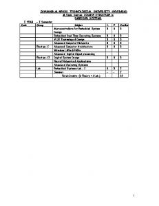
��� � � � ��� � � � � � ! " �� � � � � ��� � � � � � � � � )�� � � �� � ( �! '" �� � � � � � � #%$ � � & � ' $ � ( �� � �� � Figure 1. Model structure system, the control sybsystem and the manipulator itself. The general model structure is shown on Fig. 1. 4.1.1 Vision Subsystem
*,+ *.-
Let’s suppose that the target detection algorithm should take not more time to execute, and it runs periodically with pause time . If a target is detected, the vision subsystem sends a message with target coordinates (and velocity) to the control subsystem. Here is the model text for the vision subsystem:
4.1 Model Construction
1 message Target {}; /*message to control subsystem */ 2 process Vision() < 3 output TargetData; /* output buffer to send a message */ 4 > 5 { 6 msg TargetMark; /* message variable */ 7 /* model parameters */ 8 float Td = 1000; /*time for detection */ 9 float Tp = 200; /* pause length */ 10 while( 1 ){ 11 delay( Td ); /* simulate target detection */ 12 if( TargetDetected() ) { /* target is detected */ 13 TargetMark = message Target; 14 send( TargetMark, TargetData ); /* send message to control subsystem */ 15 } 16 delay( PauseTime ); /* do pause */ 17 } 18 } /* Vision */
The following components operating in parallel could be distinguished in our system to be modeled: the vision sub-
Note that on the current level of detail the vision subsystem is treated just like the source of messages on targets (see
4. An Example of Model Construction in DYANA The capabilities of model descriprion will be shown on en example of robotic control system for the manipulator (i.e. robot’s arm). The aim of manipulator’s work is to catch a moving oblect (a target). The manipulator consists of two chains and it has two degrees of freedom. To detect the target and to determine the target’s coordinates, a vision subsystem is provided, its particular principle of operation does not influence on this article’s subject and will not be considered. The idea of control algorithm is as follows. Having the target’s and manipulator’s coordinates a catch point is determined. Then, a trajectory of manipulator moving up to the catch point is computed. The next step is to move the manipulator along the trajectory. If the trajectory is passed and the target is not caught, new catch point is computed, and so on. To follow the trajectory, the feedback-by-error algorithm is used, which is implemented on the control computer.
the message type description in line 1, the message is sent in line 14). The target detection algorithm itself is presented by the delay in line 11, which specifies the execution time for this algorithm. There is no computations there. The possibilities of model detail will be considered later, in Sect. 4.3.
The low control level is responsible for following by computed trajectory, in presence of external physical infuences on the manipulator. Its implementation is omitted for brevity.
4.1.2 Control Subsystem
4.1.3 Manipulator
Let’s partition the control algorithm on high level and low level of control. Each level is presented by a separate process. The algorithm operates by the following way. When the high control level process receives thetarget coordinates, it requests the coordinates of manipulator and checks the possibility to catch the target. If catching is possible, the manipulator’s trajectory is computed and sent to the low control level process. These actions are repeated for the next position of target. Model text is as follows:
In our model, the manipulator can perform two operations: to determine and send its coordinates; to do an (elementary) move by the control system’s command. The Manip process may receive messages of two types: move command (Move) and request for coordinates (CoordReq). Having received the former message, Manip makes a move and sends its coordinates to the low control level. Upon receiving the latter one, it replies with coordinates to the high control level. Note that the Manip process, essentially, isn’t a part of the computer system, it’s a component of an computer system’s outer environment. Under this term we mean the set of sensors, servomechanisms etc. interfacing a computer control system with controlled object. So, building a software model in the DYANA environment opens an opportunity to investigate the program behaviour together with its outer environment, which is crucial for the real-time programs development.
1 process HiControl() < 2 input TargetData(queue), Feedback(queue); 3 output Control, ManipAcq; 4 > 5 { 6 msg in, out, x; 7 int CatchPossible; /* time to compute catch point */ 8 float ComputeCP = 100; /* time to compute trajectory */ 9 float ComputeTraj = 100; 10 11 while( 1 ) { /*get target parameters */ 12 receive( in, TargetData ); 13 out = message CoordReq; /*request for manipulator’s coordinates */ 14 send( out, ManipAcq ); /* get manipulator’s coordinates */ 15 receive( x, Feedback ); 16 /* test for possibility of catching and catch point computation */ 17 delay( ComputeCP ); 18 if( !CatchPossible ) continue; /* impossible to catch */ /* compute trajectory parameters */ 19 delay( ComputeTraj ); /* send trajectory to low control level */ 20 out = message Traj; 21 send( out, Control ); 22 } /* while */
23
} /* HiControl */
4.2 Taking Hardware Into Account Besides the program description considered above, the complete model contains: hardware description (a set of executors); �
�
process to executor binding description.
The sequential executor is an abstraction of a device performing only one action at a time. Let’s suppose that we use a dedicated signal processor for the vision subsystem and general-purpose Intel 80386based computer — for the control subsystem. Then, the hardware description in -SIM may look like:
��
sequex DSP() {} /*for vision subsystem */ sequex CPU() { /* for control subsystem */ architec Intel386; } sequex Manip() {} /*for manipulator */ Leaving some syntactical details, one of possible binding descriptions may look like:
bind bind bind bind
Vision => DSP; HiControl => CPU; LowControl => CPU; Manip => Manip;
The HiControl and LowControl processes are bound to the same executor. They will run in thr interleaved fashion. The actions of vision and Manip (these processes are bound to distinct executors) could be executed in parallel (if waiting for message does not instruct otherwise). Please note that the notion of executor could represent not only a CPU, but any other hardware component (e.g., a bus, a memory module, a switch etc). In this case, the sequential executor should be accomplished by the appropriate process containing the operation algorithm of the device to be modeled.
4.3 Model Detail. Model-to-Program Transition In order to move from a model to a program, you should refine the data structure in messages and actions in processes. For example the structure of message Target from process Vision below and the delay statement in line 17 of process HiControl (catch point calculation) could be detailed by the following way: message Target {float Xt, Yt, Zt, Vx, Vy, Vz }; complex { C1 = cos(theta1); S1 = sin(theta1); C2 = cos(theta2); S2 = sin(theta2); Xm = (l1+l2*C2)*C1; Ym = (l1+l2*C2)*S1; Zm = l2*S2; ... } The complete text of the catch point calculation is omitted due to the lack of space. Note the complex block above. If the architecture description of the target CPU is given in the model, the execution time of this block for given target CPU will be estimated during the model run. For details on time estimation, see Sect. 5.2. -SIM program is finished, it may When the detail of be converted into a C++ program for the target computer. For example, let’s see the part of the conversion result for HiControl process below.
��
#include "__mm.h" ... void __mm_process_HiControl:: __mm_process_body() { ...
__mm_message *in = new __mm_message; int CatchPossible; while(1){ __mm_receive(__mm_bf_TargetData,in, 1,"HiControl.mm:12"); (&__mm_sample_message_CoordReq)-> __mm_copy_message(out); __mm_send(__mm_bf_ManipAcq,out,2, HiControl.mm:14"); ... __mm_delay(ComputeCP,3,"HiControl.mm:17"); ... } } Of course, the details of the target operating system interface should be taken into account. But it’s not a subject of this paper. Here we want only to show the possibility of such a conversion. An important note: the DYANA environment is capable to reproduce the parallel program behaviour with respect to computer system architecture of interest and particular outer environment on any stage of model detail. So, meeting the specified deadlines in a real-time control systems could be checked on any stage of detail.
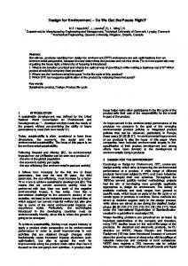
5. DYANA Architecture The architecture of the DYANA system is shown on the Fig. 2. The most interesting components of the DYANA system are described below.
I n t e g r a t e d D e v e l o p m e n t E n v i r o m e n t
������ � ��� �� �� ���� � � ��������� � � �
������ �� � � � � � � � � � � � ! " � # $ � � %&� $ ' ( $ ' � ) 6�� �7- -���- -��� � � ��� �� �� ���� � � �.� /0�.,������ � � " �.� ( 8 �.� !0(9! : ; � $ � < $ �.' ) * �� �
��� ����� + �� , � � �� �� �-� � � �.� /0�.,������ �
Database
3��-�-�� � �
�� �-� � � �
4���� �� �� � �.� /���,�� ��� �
3� �.� ��� 5��-� � � �.� /0�.,������ �
=��-� 2�� �������- � � �-� �� -��, �
Figure 2. Architecture of the DYANA system
1 �-�-
�2� ���� � � ����/0��,�� ��� �
5.1 The Runtime Subsystem The runtime subsystem is responsible for the following: reproduction of the system’s behaviour on the base of process-oriented discrete-event simulation methodology (before execution, the program description in SIM is translated to the text in the C language, compiled and linked with the DYANA runtime library); �
��
�
collection of the event trace for subsequent analysis. Also, the dynamic stage of the time estimation (see 5.2) is done by the runtime subsystem. Now, the design and development of distributed discrete-event simulation kernel for DYANA is in progress. Our approach to analysis and choozing the distributed model time synchronization algorithm is presented in [8].
5.2 The Subsystem for Time Complexity Estimation On the early stages of the model development, action of a process is not detailed up to the actual computation block. So it may be specified by its time delay1 . When a model is being detailed the delay statements are being replaced by actual code blocks. It’s worth to preserve the capability of timing a model ’automatically’ during its detailing. The aim of this subsystem is to estimate an execution time of a text block in the C language in the complex statements for given target CPU architecture. The underlying theory and architecture of this subsystem were described in [7, 13]. Briefly, the main idea is as follows. The combined static-and-dynamic approach is used for the time estimation purposes. During compilation, static analysis of the C code is being performed. For every linear code block in complex statement a prediction of execution time is being made. During a model run, when exact sequence of executed linear code blocks is known, the time estimate is being given on the base of static predictions. The mapping of computations to the target CPU architecure is implemented by the following way. A model of CPU architecture is being constructed which captures the essential features of a certain archtecture class, influencing on the execution time. For example, models of an von-Newmann sequential register-stack CPU and of a RISC CPU are supported now. For the register-stack CPU model. the algorithms of optimal code generation are implemented. The execution time estimate is based on the length of code generated [7]. During testing, the relative error of execution time prediction 1 The delay for a message transfer could be represented as by constant link speed placed in the executor description as by the model of the communicational channel
was in range of four to ten percents which is acceptable for practical use. The RISC CPU model enables you to determine statically the pipeline latencies due to data dependencies in instructions. Also, the instruction cache behaviour analysys could be done in the static phase. The architecture type of sequential can be specified by writing an identifier of the architecture, as follows: architec Intel286; The architecture description itself (it can be rather awkward) is placed separately and specifies the clock rate, register structure and instruction set of an executor. For RISC processors this description contains also the pipelines structure, instruction processing scheme and cache configuration.
5.3 The Visualization Subsystem This subsystem is intended to view the event trace collected during model run. Events are associated with interprocess communication and with the beginning and finishing of process internal actions. The collected trace could be viewed in the form of timing diagram. User is able to scroll and scale the diagram, to select the model components of interest for visualization, to get an additional information about event and state attributes by clicking on event (state). Also, an important feature is the capability to observe the logical links between events and to locate the corresponding piece of process’s text while browsing events.
5.4 The Performance Analysis Subsystem This subsystem is useful when you need certain integrated performance indices (such as working time, idle time, processor utilization, message queue length etc). These indices can be computed and displayed as tables, graphs and histograms. The output data representation enables import into Microsoft Excel for advanced processing and report generation.
5.5 The Algorithmic Analysis Subsystem This subsystem allows the user to specify the behaviour of software under development and to verify the software behaviour against specification. Under term ’behaviour’ we mean the partially ordered set of events (See [12] for details). The approach to specification and verification (with the previous version of this language) was described in [15]. For the specification of properties of system being modeled, a special language was developed. This language named -SPEC permits:
�
to specify the actions of a process as relations between process states before and after an action; �
to specify possible chains of actions using behavior expressions; �
�
to specify the properties of a process and a whole system behavior as predicates on behavior expressions;
��
For example, the following valuable program properties -SPEC : the absence of could be specified by means of a deadlock, the proper reaction on a certain stimulus for any program history and for any timing. An important feature of -SPEC is: its syntax is close to one of -SIM , but the semantics of -SPEC is equivalent to one of the branching time logic. For the following two problems algorithms are developed and prototyped now: checking the consistency of specification itself; verifying the specification against the model description on the -SIM . More detailed description of the -SPEC could be found in [4]. For our methods of verification, please refer to [17].
��
� �
��
��
5.6 The Integrated Development Environment 5.6.1 Notes on Technology of Model Development
�
As we have noted above, one of the goals of -SIM development is to support the top-down design. That is, to let the user to start from the large-grain model picking up only general structure of system to be simulated and ignoring small-grain details. Gradually, step-by-step small details are refined, more and more detailed models are developed. Such an stepwise detail should be performed in three directions. 1. Structure detail implies the detail of component’s internal structure. Such a feature is provided by independence of the distributed programs and the executors description on internal structure of subcomponents. Because of modularity, changes in any part of the model does not require changing (and even recompiling) of other parts. 2. Action detail (i.e. move from simple prototyping of a process interface to real data processing). This kind of detail is provided by two ways to time complexity specification — the delay statement (it sets the model time delay explicitly but specify no computations) and the complex statement (it specifies computations, and model time delay is estimated by the special subsystem). 3. Message type and structure detail (i.e., for example, going from checking message type only to analysis of
message contents). To support such a detail, there exist two families of operators on msg-variables — the former use message type only, the latter group provide an access to message fields. 5.6.2 Integrated Development Environment Features For increasing of efficiency of model building a special object-oriented instrumental environment was developed. This object-oriented IDE relieves the user from necessity of working with files. All objects are stored in the repository (database). Every object has a visual representation on screen. All objects are arranged into the hierarchy. Models are at the top level of this hierarchy. By means of the Model List window, the user can operate on the model as a single object (e.g. compile, run it). Objects forming a model fall to one of the following groups: source descriptions, internal representations, results of model run. For every type of model component (process, executor, message etc.), the IDE handles (and gives the user to operate on) the components lists. A model component could be viewed and edited in different forms by user wish. Now textual and structural (schematic) presentations are supported. The main advantages of environment described above are as follows: 1. The usage of database provides the correspondence of external representation (e.g. screen images) of the set of descriptions with their internal organization. 2. the semantical and time dependencies between source text components could be watched more accurately, which reduce the overheads during assembling compiled model. We should highlight an important feature of developed environment — the interface description of a component can be combined with more than one version of component implementation, the implementations may be either sequential or parallel. This feature lets: 1. to perform the stepwise detail, with possibility to get back to earlier stages of development at any time; 2. to experiment with different configurations of developed and debugged model (e.g. with different versions of components implementations), what is the final goal of the user of simulation system.
6. Conclusion The DYANA environment described in this paper is aimed at the following:
description of software and hardware (on the systems level) with variable degree of detail; �
analysis of various aspects of computer system’s behaviour without hardware prototyping. �
The DYANA environment enables the user as to develop programs through simulation as to choose the proper hardware configuration. For our point of view, the most interesting features of the project are as follows: the duality of analysis methods; �
the time complexity estimation which helps to avoid the target architecture emulation. �
Now the prototype system is implemented in the Sun Solaris environment. The DYANA system is being used in the following projects: performance analysis of local area networks; �
simulation of embedded multiprocessor system for digital signal processing. �
The time complexity estimation methodology described in Section 5.2 was applied to the Motorola DSP96002 CPU. In the class of digital signal processing algorithms, a zero time prediction error was achieved, while the prediction time was 3 orders of magnitude less than emulation time (see [5]). The DYANA system is being used in the EEC INCOCopernicus Project DRTESY 2 which is aimed at evaluation (and mutual enhancement) of tools provided by project partners on a common realistic case study from the field of embedded avionics system design. Much attention will be paid to the time complexity reduction of our algorithmic analysis methods. Also, the nearest goals of future work are: to spread the database approach to trace storage and processing; �
to develop the library of CPU models for those RISC processors which are widely used in embedded computer systems; �
�
to build a library of reusable ’basic blocks’ suitable for modelling of networks and embedded hardware and software components; 2 http://www.first.gmd.de/
drtesy/
References [1] ObjecTime Limited home page, http://www.objectime.com. [2] Ptolemy simulation project home page, http://ptolemy.eecs.berkeley.edu. [3] Telelogic home page, http://www.telelogic.se. [4] Y. Bakalov and R. Smeliansky. -SPEC : A language for distributed program behaviour specification. In PARCELLA96, Berlin, 1996. [5] V. Balashov, A. Kapitonova, V. Kostenko, R. Smeliansky, and N. Youshchenko. Modelling of digital signal processors based on the static-dynamic approach. In 1st Int. Conf Digital Signal Processing and its Applications, Moscow, Russia, 1998. June, 30th – July, 3rd. [6] A. Ferscha and J. Johnson. N-MAP: A virtual processor discrete event simulation tool for performance prediction in CAPSE. In Proc. of the HICCS28. IEEE Computer Society Press, 1995. [7] A. Kapitonova, I. Terehov, and R. Smeliansky. On the computational work measure. MSU Press, Moscow, 1989. (in Russian). [8] Y. Kazakov and R. Smeliansky. Organization of synchronization algorithms in distributed simulation. In Proc. of 2nd Russian-Turkish seminar New High Information Technologies, Gebre, Turkey, May 9-12 1994. [9] T. Lewis. The next 10,0002 years. Computer, pages 64–71, April 1996. [10] M. Rosenblum and et.al. Using the SimOS machine simulator to study complex computer systems. ACM Trans. on Modelling and Computer Simulation, 7(1):78–103, January 1997. [11] B. Selic, G. Gullelson, J. McGee, and I. Engelberg. ROOM: An object-oriented methodology for developing real-time systems. In Proc. 5th International Workshop on CASE, Montreal, Canada, 1992. [12] R. Smeliansky. Distributed computer system operation model. Moscow University Computational Mathematics and Cybernetics, (3):4–16, 1990. [13] R. Smeliansky. The distributed computer systems performance estimation on the basis of program behaviour invariant, 1990. Thesis of Doctoral Dissertation, Moscow State Univ. (in Russian). [14] R. Smeliansky. Program behavior invariant as the basis for system performance estimation. In Conference on Parallel Computing Technologies, Obninsk, Russia, September 1993. [15] R. L. Smeliansky, Y. P. Kazakov, and Y. V. Bakalov. The combined approach to the distributed computer system simulation. In Conference on Parallel Computing Technologies, Novosibirsk, September 1991. Scientific Centre. [16] O. Tanir and S.Sevinc. Defining reguirements for a standart simulation environment. Computer, pages 28–34, February 1994. [17] V. Zakharov and D. Tsarkov. Efficient algorithms for the model checking in CTL and it application to the verification of parallel programs. Programming, (4):3–18, 1998.
��