Dynamic arrest within the self-consistent ... - APS Link Manager

PHYSICAL REVIEW E 76, 041504 共2007兲

Dynamic arrest within the self-consistent generalized Langevin equation of colloid dynamics

1

L. Yeomans-Reyna,1 M. A. Chávez-Rojo,2 P. E. Ramírez-González,3 R. Juárez-Maldonado,3 M. Chávez-Páez,3 and M. Medina-Noyola3

Departamento de Física, Universidad de Sonora, Boulevard Luis Encinas y Rosales, 83000, Hermosillo, Sonora, México 2 Facultad de Ciencias Químicas, Universidad Autónoma de Chihuahua, Venustiano Carranza S/N, 31000 Chihuahua, Chihuahua, México 3 Instituto de Física “Manuel Sandoval Vallarta,” Universidad Autónoma de San Luis Potosí, Álvaro Obregón 64, 78000 San Luis Potosí, SLP, México 共Received 16 February 2007; revised manuscript received 26 July 2007; published 22 October 2007兲 This paper presents a recently developed theory of colloid dynamics as an alternative approach to the description of phenomena of dynamic arrest in monodisperse colloidal systems. Such theory, referred to as the self-consistent generalized Langevin equation 共SCGLE兲 theory, was devised to describe the tracer and collective diffusion properties of colloidal dispersions in the short- and intermediate-time regimes. Its self-consistent character, however, introduces a nonlinear dynamic feedback, leading to the prediction of dynamic arrest in these systems, similar to that exhibited by the well-established mode coupling theory of the ideal glass transition. The full numerical solution of this self-consistent theory provides in principle a route to the location of the fluid-glass transition in the space of macroscopic parameters of the system, given the interparticle forces 共i.e., a nonequilibrium analog of the statistical-thermodynamic prediction of an equilibrium phase diagram兲. In this paper we focus on the derivation from the same self-consistent theory of the more straightforward route to the location of the fluid-glass transition boundary, consisting of the equation for the nonergodic parameters, whose nonzero values are the signature of the glass state. This allows us to decide if a system, at given macroscopic conditions, is in an ergodic or in a dynamically arrested state, given the microscopic interactions, which enter only through the static structure factor. We present a selection of results that illustrate the concrete application of our theory to model colloidal systems. This involves the comparison of the predictions of our theory with available experimental data for the nonergodic parameters of model dispersions with hard-sphere and with screened Coulomb interactions. DOI: 10.1103/PhysRevE.76.041504

PACS number共s兲: 64.70.Pf, 61.20.Gy, 47.57.J⫺

I. INTRODUCTION

The dynamic properties of colloidal dispersions have been a subject of sustained interest for many years 关1–3兴. These properties can be described in terms of the relaxation of the fluctuations ␦n共r , t兲 of the local concentration n共r , t兲 of colloidal particles around its bulk equilibrium value n. The average decay of ␦n共r , t兲 is described by the time-dependent correlation function F共k , t兲 ⬅ 具␦n共k , t兲␦n共−k , 0兲典 of the FouN rier transform ␦n共k , t兲 ⬅ 共1 / N兲兺i=1 exp关ik · ri共t兲兴 of the fluctuations ␦n共r , t兲, with ri共t兲 being the position of particle i at time t. F共k , t兲 is referred to as the intermediate scattering function, measured by experimental techniques such as dynamic light scattering. One can also define the selfcomponent of F共k , t兲, referred to as the self-intermediate scattering function, as FS共k , t兲 ⬅ 具exp关ik · ⌬R共t兲兴典, where ⌬R共t兲 is the displacement of any of the N particles over a time t. In recent work a self-consistent theory of colloid dynamics has been developed 关4–9兴, leading to the first-principles calculation of the dynamic properties above. This scheme allows the calculation of F共k , t兲 and FS共k , t兲, given the effective interaction pair potential u共r兲 between colloidal particles and the corresponding equilibrium static structure, represented by the radial distribution function g共r兲 or the static structure factor S共k兲. This theory, referred to as the selfconsistent generalized Langevin equation 共SCGLE兲 theory, is based on general and exact expressions 关4兴 for F共k , t兲 and 1539-3755/2007/76共4兲/041504共15兲

FS共k , t兲 in terms of a hierarchy of memory functions, derived within the generalized Langevin equation 共GLE兲 approach and the process of contraction of the description 关10,11兴, and complemented by a number of physically or intuitively motivated approximations 关5,6兴. A systematic assessment of the intrinsic accuracy and limitations of the resulting approximate scheme under the simplest possible conditions 共model monodisperse suspensions of spherical particles with no hydrodynamic interactions兲 has also been presented 关7兴. This was based on the comparison of the theoretical predictions for specific idealized model systems, with the corresponding Brownian dynamics computer simulation data in the shortand intermediate-time regimes. The same theoretical scheme has also been extended to describe the dynamics of colloidal mixtures 关8,9兴. The theoretical infrastructure just described is now being applied to study specific systems or phenomena. The main purpose of the present paper is to address the issue of its capability to describe the ideal ergodic-nonergodic transition in simple model colloidal systems. The fundamental understanding of dynamically arrested states of matter is one of the most fascinating topics of condensed matter physics, and several issues related to their microscopic description are currently a matter of discussion 关12–14兴. Among the various approaches to the understanding of the transition from an ergodic to a dynamically arrested state, the mode coupling 共MC兲 theory 关14–17兴 provides perhaps the most comprehensive and coherent picture. In fact, a large number of experimental observations in specific sys-

041504-1

©2007 The American Physical Society

PHYSICAL REVIEW E 76, 041504 共2007兲

YEOMANS-REYNA et al.

tems, particularly in the domain of colloidal systems 关18–22兴, seem to agree with the predictions of this theory. The mode coupling theory of the ideal glass transition emerged originally in the framework of the dynamics of molecular 共not colloidal兲 liquids 关16,17兴. Although one can expect 关23兴 that the phenomenology of dynamic arrest does not depend on the short-time motion 共which distinguishes between molecular and colloidal dynamics兲, it is convenient to base a theory for the glass transition of colloidal systems on the diffusive microscopic dynamics characteristic of these systems. In fact, in 1983 Hess and Klein 关2兴 proposed the translation of the mode coupling self-consistent theory from the molecular context to colloidal systems, and extensive calculations based on such theory were eventually reported in the literature 关24兴. More recently, Nägele and collaborators developed a more elaborate version of this theory 关25兴. This scheme has been successfully extended and applied in several interesting directions 关26兴, and the level of its quantitative accuracy at short and intermediate times has been documented 关27,28兴, as well as its capability to predict the same scenario of dynamic arrest as the original MC theory 共MCT兲. The SCGLE theory that we shall discuss in this paper shares with the colloid-dynamics version of MCT developed by Nägele and collaborators 关25兴 a number of important features. Most notably, both were developed with the intention to describe accurately the short- and intermediate-time dynamics of colloidal systems. They, however, differ radically in the conceptual framework upon which they are built. Thus, our theory is certainly not another version of MCT, and differs also from recent variants 关29,30兴 of MCT mainly aimed at improving the performance of the original theory concerning the description of the ideal glass transition. Similarly, there is no direct relationship between the conceptual basis of the present theory and that of other theories of colloid dynamics partially or fully based on kinetic-theoretical concepts 关31,32兴. For this reason, one important aim of the present paper is to summarize the basic ingredients of the derivation of our theory. The description of the transition to arrested states involves a large number of issues, which must be addressed systematically. One of the most crucial ones refers to the derivation of practicable, first-principles methods, to predict the location of the boundary between the ergodic and the arrested states of a system, given the effective forces between particles. In this paper we focus on this particular issue, which is the nonequilibrium analog of the statistical thermodynamic derivation of equilibrium phase diagrams. In principle, the set of coupled nonlinear dynamic equations that constitute the self-consistent theory must contain this information, and its numerical solution is the “brute force” but safer route to reveal it. In this paper, besides numerically solving the full self-consistent theory for the space and time dependence of all the dynamic properties involved, we focus on the derivation of a more direct criterion that allows us to locate the transition to dynamically arrested states in a much simpler manner. This criterion consists of an equation for the nonergodic parameters, which are the long-time asymptotic values of the various dynamic properties involved, whose nonzero value is the signature of the glass state. Just as in MCT 关14兴, this

equation is derived from the long-time analysis of the selfconsistent theory. In the present case, however, the resulting equations are reduced to a closed equation for a single scalar parameter, namely, the long-time value of the mean squared displacement of a tagged particle, that we denote as ␥. This parameter has a finite value in the arrested state, and is infinite in the ergodic fluid state. Such an equation involves only the static structure factor S共k兲 as an input. The solution of this equation allows then the determination of the wavevector dependent collective nonergodic parameter f共k兲 associated to the arrest of concentration fluctuations, which are written in a remarkably simple explicit expression that only involves S共k兲 and ␥. We would like to stress that the main contribution of this paper is not some specific quantitative advantage of the theory presented, over MCT or other descriptions of dynamic arrest. Instead, the main contribution is the proposal of an alternative and independent perspective to model the glass transition. The expectation is that this alternative theoretical framework will join other approaches, most notably MCT, in the effort to improve our understanding and our predictive capability regarding dynamic arrest phenomena. We do expect, however, that the practical application of our selfconsistent scheme will prove to be somewhat simpler than the use of MCT equations, and that this will facilitate its use by other people. For example, the extension of our theory to mixtures is rather straightforward, and this will allow its application to many specific systems and phenomena. In order to explain these advances, however, a preliminary step is to present the fundamental basis of our theory and to illustrate its application in the context of the simplest and most paradigmatic systems and phenomena; this is the main purpose of the present paper, which is explicitly limited to the context of monodisperse systems. Furthermore, in this paper we do not consider the effects of hydrodynamic interactions, which are fundamental in the discussion of the dynamic properties at short and intermediate times. As a working hypothesis, in this paper we shall assume that hydrodynamic interactions will not influence in a qualitative and fundamental manner the asymptotic long-time dynamics of the colloidal dispersion near its transition to dynamic arrested states nor the corresponding “phase diagram.” This paper is organized as follows. In the following section and in two appendixes we describe our self-consistent generalized Langevin equation 共SCGLE兲 theory for colloid dynamics, and discuss very briefly the physical content and the rationale of each of the approximations involved in its formulation. In order for this paper to be reasonably selfcontained, this will involve a certain degree of repetition with respect to Refs. 关4–6,10兴, which contain all the details of its derivation and in which the quantitative accuracy of the most essential approximations of our theory is explicitly monitored. In Sec. III we derive the equations for the nonergodic parameters, and illustrate the manner in which this criterion is employed in the context of the hard-sphere system. In Sec. IV we present the numerical solutions of the full self-consistent theory for the time and wave-vector dependence of the intermediate scattering function of the same reference system. In Sec. V we present an illustrative selection of comparisons of the results of the present theory with

041504-2

DYNAMIC ARREST WITHIN THE SELF-CONSISTENT …

PHYSICAL REVIEW E 76, 041504 共2007兲

those measured in two experimental model systems. The first is the suspension of colloidal hard spheres, for which the transition is theoretically-predicted to occur at a volume fraction of ␾g = 0.563, in very close agreement with reported experimental results. The second is a colloidal suspension of charged particles. In Sec. VI we present particular details and limiting conditions concerning the Vineyard-like approximations introduced in this work. In Sec. VII we discuss and summarize our main results.

subject of Ref. 关4兴. As a result, one obtains the most general expression for F共k , t兲 and FS共k , t兲 that describes the dynamics of the suspension in the diffusive regime 共i.e., for times t Ⰷ ␶B兲. In Laplace space, the resulting “overdamped” expressions for F共k , z兲 and FS共k , z兲 read 关4兴 F共k,z兲 =

S共k兲 k D0S−1共k兲 z+ 1 + C共k,z兲

共2.1兲

1 , k 2D 0 z+ 1 + CS共k,z兲

共2.2兲

2

and II. SELF-CONSISTENT GLE THEORY

The development of the self-consistent generalized Langevin equation theory involves four distinct fundamental elements 关6兴. The first consists of general and exact expressions for F共k , z兲 and FS共k , z兲 关the Laplace transforms of F共k , t兲 and FS共k , t兲, respectively兴, in terms of a hierarchy of memory functions. The second element consists of the formalization of the notion that collective dynamics should somehow be simply related to self-dynamics. This notion reduces the problem of colloid dynamics to the independent determination of FS共k , z兲 itself, or of its memory function CS共k , t兲. The third basic element of our theory is the proposal for the approximate determination of CS共k , t兲. This step is based on the physically intuitive expectation that spacedependent self-diffusion, represented by FS共k , t兲, should be simply related to the properties that characterize the Brownian motion of individual particles, such as the mean squared displacement. The fourth ingredient of the theory is provided by an independent expression for ⌬␨共t兲, the time-dependent friction function that embodies the effects of interparticle interactions on the Brownian motion of individual tracer particles, and which can be approximately written in terms of F共k , t兲 and FS共k , t兲, thus constituting a final closure of our fully self-consistent theory of colloid dynamics. Let us now review each of these four elements in some more detail. In Ref. 关4兴 the GLE approach and the concept of the contraction of the description 关10,11兴 were employed to derive the most general time-evolution equation for the fluctuations ␦n共r , t兲 of a monodisperse colloidal suspension in the absence of hydrodynamic interactions. In such derivation, the assumed underlying microscopic N-particle dynamics was provided by the many-particle Langevin equation 关1兴. As a result, expressions were derived for F共k , t兲 and FS共k , t兲 关or their Laplace transforms F共k , z兲 and FS共k , z兲兴 in terms of a hierarchy of memory functions, and of welldefined static structural properties of the Brownian fluid. In these expressions, the Brownian relaxation time ␶B ⬅ M / ␨0 共or the corresponding frequency zB ⬅ ␶B−1兲 appears, where M and ␨0 are, respectively, the mass and the solvent-friction coefficient of each particle in the suspension. In the absence of friction 共␨0 → 0兲, these expressions correspond to those of a simple atomic liquid 关33,34兴. In the presence of friction, and in order to “tune” these expressions to the time regime normally probed by dynamic light scattering experiments or by Brownian dynamics simulations, the limit t Ⰷ ␶B, or z Ⰶ zB, must be taken. Taking this so-called “overdamping” limit 关4兴 requires a careful analysis, which was the main

FS共k,z兲 =

where C共k , z兲 and CS共k , z兲 are the respective memory functions. We should mention that these results are exact, and can be derived in a variety of manners. They can be derived, for example, from the N-particle Smoluchowski dynamics using the projection operator formalism, C共k , z兲 and CS共k , z兲 being referred to as the “irreducible memory functions” 关25,26兴. These general results constitute the starting point of the MCT, and they are also the basis of our present SCGLE theory. In our case, however, the generalized Langevin equation approach also provides exact expressions for the irreducible memory functions in terms of higher-order memory functions denoted by ⌬L共k , z兲 and ⌬LS共k , z兲, namely, C共k,z兲 =

z + 关␹

*

k2D0␹*共k兲 共2.3兲 + 关␹*共k兲兴−1⌬L*共k,z兲

共k兲兴−1L*0共k兲

and CS共k,z兲 =

k2D0␹*S共k兲 * z + 关␹*S共k兲兴−1L0S 共k兲 + 关␹*S共k兲兴−1⌬L*S共k,z兲

. 共2.4兲

In these equations, D0 = kBT / ␨ is the free-diffusion coefficient of each particle 共kBT being the thermal energy兲, S共k兲 the static structure factor, and ␹*共k兲 the static correlation function of the fluctuations of the configurational component of the stress tensor of the Brownian fluid. ␹*共k兲 and L*0共k兲, * along with their self-counterparts ␹*S共k兲 and L0S 共k兲, are static properties, which can be written exactly 关see Eqs. 共A1兲–共A3兲 of Appendix A兴 in terms of the two- and three-particle correlation functions, g共r兲 and g共3兲共r , r⬘兲, which are assumed to be known. In practice, the use of Kirkwood’s superposition approximation allows us to write these properties in terms only of g共r兲 关see Eq. 共A6兲兴. Thus, the only unknown properties in the expressions for F共k , t兲 and FS共k , t兲 in Eqs. 共2.1兲–共2.4兲 are the memory functions ⌬L*共k , z兲 and ⌬L*S共k , z兲. Neglecting ⌬L*共k , z兲 and ⌬L*S共k , z兲 in Eqs. 共2.3兲 and 共2.4兲 leads to the so-called single exponential 共SEXP兲 approximation 关35,36兴, which consists of Eqs. 共2.1兲 and 共2.2兲 with 0

C共k,z兲 ⬇ CSEXP共k,z兲 ⬅ and

041504-3

k2D0␹*共k兲 z + 关␹*共k兲兴−1L*0共k兲

共2.5兲

PHYSICAL REVIEW E 76, 041504 共2007兲

YEOMANS-REYNA et al.

CS共k,z兲 ⬇ CSEXP 共k,z兲 ⬅ S

k2D0␹*S共k兲

z+

. * 关␹*S共k兲兴−1L0S 共k兲

共2.6兲

This approximation is exact at short times and/or large wave vectors, an important fact employed below. As the second ingredient of the self-consistent theory, we search for a simple approximate relation between collective and self-dynamics. Vineyard’s approximation 关37兴, which relates F共k , t兲 directly to FS共k , t兲 as F共k , t兲 ⬇ FS共k , t兲S共k兲, is a simple 共although qualitatively and quantitatively rather primitive 关33,34兴兲 implementation of this idea. Our proposal is, instead, to relate the memory function of F共k , t兲 with the corresponding memory function of FS共k , t兲. In Ref. 关5兴, a detailed numerical study of alternative such manners to refer collective dynamics to self-diffusion was carried out. Equations 共2.1兲–共2.4兲 suggest to relate F共k , z兲 and FS共k , z兲 at the level of their highest-order memory functions. It was found, indeed, that a very accurate approximation was * 共k兲. In practice, however, it ⌬L*共k , z兲 / L0共k兲 = ⌬L*S共k , z兲 / L0S was also found 关5兴 that equally precise connections could also be achieved at the level of the second-order memory functions C共k , z兲 and CS共k , z兲. Two specific proposals of such Vineyard-like approximations were considered 关6,9兴, which can be written in the generic form C共k,z兲 = w共k,z兲CS共k,z兲 + y共k,z兲,

共2.7兲

with w共k , z兲 and y共k , z兲 being known functions. The first approximates the ratio C共k , z兲 / CS共k , z兲 by its SEXP value, C共k,z兲 =

冋

CSEXP共k,z兲 CSEXP 共k,z兲 S

册

level of their respective memory functions. The memory function of W共t兲 is the so-called time-dependent friction function ⌬␨共t兲. Although we do not have a physically transparent notion to guide us, we know, however, two exact limits that CS共k , t兲 must satisfy. Thus, for large wave vectors CS共k , t兲 is given exactly by CSEXP 共k , t兲, whereas for small S wave vectors CS共k , t兲 is given exactly by the time-dependent friction function ⌬␨共t兲. This function, normalized by the solvent friction ␨0, is essentially the memory function of the velocity autocorrelation function. In Ref. 关6兴 it was proposed to interpolate CS共k , t兲 between these two exact limits by means of the following expression: 共k,t兲 + 关⌬␨*共t兲 − CSEXP 共k,t兲兴␭共k兲, CS共k,t兲 = CSEXP S S 共2.10兲 where ⌬␨*共t兲 ⬅ ⌬␨共t兲 / ␨0, and ␭共k兲 is a phenomenological interpolating function, such that ␭共k → 0兲 → 1, and ␭共k → ⬁兲 → 0. The detailed functional form of this interpolating function will be described shortly. The last ingredient of our theory is an expression for the time-dependent friction function ⌬␨*共t兲. For this property, a general and exact result has also been derived 关10兴 within the framework of the GLE approach; the corresponding derivation is summarized in Appendix B. Such an exact result, however, can be simplified by means of well-defined approximations 关10兴, also indicated in Appendix B, to read ⌬␨*共t兲 ⬅

CS共k,z兲,

共2.8兲

where the SEXP memory functions are given by Eqs. 共2.5兲 and 共2.6兲. This is referred to as the “multiplicative” Vineyard-like approximation, and corresponds to w共k , z兲 共k , z兲兴 and y共k , z兲 = 0. The second ap= 关CSEXP共k , z兲 / CSEXP S proximates the difference 关C共k , z兲 − CS共k , z兲兴 by its SEXP value, and is referred to as the “additive” Vineyard-like approximation. It is defined by w共k , z兲 = 1 and y共k , z兲 共k , z兲兴, i.e., = 关CSEXP共k , z兲 − CSEXP S 共k,z兲兴. C共k,z兲 = CS共k,z兲 + 关CSEXP共k,z兲 − CSEXP S

共2.9兲

Later on we shall discuss the merits and deficiencies of these two specific proposals. Either of them, however, refer collective dynamics to self-dynamics, represented by the irreducible memory function CS共k , z兲. Thus, we must search for some form of approximation for this memory function. The third ingredient of the present theory consists of the proposal for the approximate determination of CS共k , t兲. One intuitively expects that these properties should be simply related to the properties that describe the Brownian motion of individual particles, just like in the Gaussian approximation 关1,2兴, which expresses FS共k , t兲 in terms of the mean squared displacement W共t兲 as FS共k , t兲 = exp关−k2W共t兲兴. The present self-consistent theory introduces an analogous approximate connection between the functions FS共k , t兲 and W共t兲, but at the

⌬␨共t兲 D 0n = ␨0 3共2␲兲3

冕 冋 dk

kh共k兲 1 + nh共k兲

册

2

F共k,t兲FS共k,t兲, 共2.11兲

where h共k兲 = 关S共k兲 − 1兴 / n. This approximate expression for ⌬␨*共t兲 is one of the most important ingredients of the present theory. Let us mention that exactly the same expression was first introduced to the context of colloid dynamics by Hess and Klein 关6兴, with arguments borrowed from mode coupling theory. As it is apparent from the derivation in Appendix B, our derivation follows a completely independent line of reasoning, and provides possible systematic manners to relax the approximations involved. A closed system of equations results from all the arguments and approximations above, which can be summarized by the exact results in Eqs. 共2.1兲 and 共2.2兲, complemented with either of the Vineyard-like approximations of the generic form in Eq. 共2.7兲, plus the interpolating formula in Eq. 共2.10兲, along with the closure relation for the time-dependent friction function in Eq. 共2.11兲. All the elements entering in these equations, including the SEXP approximation for the memory functions in Eqs. 共2.5兲 and 共2.6兲, involve only static properties, which can be determined by the methods of equilibrium statistical thermodynamics, given the potential u共r兲 of the pairwise forces between the particles. Concerning the interpolating function ␭共k兲, a functional form of the general type ␭共k兲 = 关1 + 共k / kc兲␯兴−1 was proposed 关6兴, and the choice of the parameters kc and ␯ was made by comparing the theoretical predictions for various values of kc and ␯ with exact

041504-4

DYNAMIC ARREST WITHIN THE SELF-CONSISTENT …

PHYSICAL REVIEW E 76, 041504 共2007兲

共computer simulated兲 data for a particular model system, at a given state, and at a given time. This led to the following prescription for ␭共k兲, 1

␭共k兲 = 1+

冉 冊 k

共2.12兲

2,

kmin

where kmin is the position of the first minimum of the static structure factor S共k兲 of the system. This turns out to be an excellent interpolating device for all systems considered so far. Although no fundamental basis is available for this choice of ␭共k兲, this definition is universal 共in the sense that it is the same for any system or state兲, and renders the resulting self-consistent scheme free from any form of adjustable parameters. Since this self-consistent theory was not conceived within the theoretical framework of mode coupling theory 共MCT兲, it makes little sense to define it in terms of a certain choice of the so-called vertex function, i.e., the specific manner in which the memory functions C共k , z兲 and CS共k , z兲 are expressed in terms of F共k , z兲 and FS共k , z兲 themselves. In our case, however, we may say that such a relation is contained in the 共multiplicative or additive兲 Vineyard-like approximation, Eq. 共2.7兲, plus the closure relation for CS共k , z兲 in terms of the time-dependent friction function in Eq. 共2.10兲, along with the approximate expression in Eq. 共2.11兲 for ⌬␨*共t兲 in terms of the intermediate scattering functions. We should mention that the general scenario of the ideal glass transition provided by our theory at this level of approximation, however, seems to be remarkably similar to that predicted by the MCT concerning, for example, the qualitative phenomenology of the relaxation of F共k , t兲 and FS共k , t兲 near the transition, as illustrated below with the full solution of this selfconsistent system of equations. Before that, however, let us discuss the prediction of the theory regarding the location of the boundary between ergodic and nonergodic states. III. NONERGODIC PARAMETERS AND THE LOCATION OF THE GLASS TRANSITION

In this section we derive a criterion that allows us to locate the glass transition in a particularly simple manner, us-

⌬␨*共⬁兲 =

D 0n 3共2␲兲3

冕

dk

ing only the static structure factor as an input. This criterion is the prediction of our theory concerning the long-time asymptotic value of the various dynamic properties. For the intermediate scattering function, f共k兲 ⬅ limt→⬁ F共k , t兲 / S共k兲 is referred to as the nonergodic parameter. Here we also define c共k兲 ⬅ limt→⬁ C共k , t兲, cS共k兲 ⬅ limt→⬁ CS共k , t兲, and ⌬␨*共⬁兲 ⬅ limt→⬁ ⌬␨*共t兲. The nonzero value of these nonergodic parameters is a signature of the glass state. The equation that determines ⌬␨*共⬁兲 constitutes the criterion referred to above. To derive this criterion, let us substitute the dynamic properties above, involved in the self-consistent system of equations in Eqs. 共2.1兲, 共2.2兲, and 共2.9兲–共2.11兲, by the sum of their asymptotic long-time value plus the rest 共which, by definition, always relaxes to zero兲. In the resulting system of equations, let us now take the asymptotic long-time limit, thus generating the following self-consistent system of equations for the “nonergodic” parameters of the properties involved: f共k兲 =

c共k兲 , c共k兲 + k2D0S−1共k兲

共3.1兲

cS共k兲 , cS共k兲 + k2D0

共3.2兲

f S共k兲 =

c共k兲 = w共k兲cS共k兲,

共3.3兲

cS共k兲 = ␭共k兲⌬␨*共⬁兲 ,

共3.4兲

and ⌬␨*共⬁兲 =

D 0n 3共2␲兲3

冕

dk

关kh共k兲兴2 f共k兲f S共k兲, 1 + nh共k兲

with w共k兲 ⬅ w共k , z = 0兲. Using Eqs. 共3.3兲 and 共3.4兲 in Eqs. 共3.1兲 and 共3.2兲, we can express the nonergodic parameters f共k兲 and f S共k兲 in terms of ⌬␨*共⬁兲. Substituting the resulting expressions in Eq. 共3.5兲, we finally obtain the following closed equation for ⌬␨*共⬁兲:

关kh共k兲␭共k兲⌬␨*共⬁兲兴2w共k兲 . 关1 + nh共k兲兴关w共k兲␭共k兲⌬␨*共⬁兲 + k2D0S−1共k兲兴关␭共k兲⌬␨*共⬁兲 + k2D0兴

Clearly, this equation always admits the trivial solution ⌬␨*共⬁兲 = 0, which corresponds to the ergodic fluid state. The existence of other nonzero real solution共s兲 is associated to the glass state. The ideal glass transition is located at the boundary of the region where this equation ceases to have real solutions other than the trivial ergodic solution. In practice, we eliminate the trivial solution by dividing Eq. 共3.6兲 by ⌬␨*共⬁兲, and rewriting it as

共3.5兲

⌽关␥ ;S兴 ⬅

1 6 ␲ 2n

= 1,

冕

⬁

0

dkk4

共3.6兲

关S共k兲 − 1兴2␭2共k兲w共k兲␥ 关w共k兲␭共k兲S共k兲 + k2␥兴关␭共k兲 + k2␥兴 共3.7兲

with ␥ defined as ␥ ⬅ D0 / ⌬␨*共⬁兲. That ␥ is the mean squared displacement can be seen from the fact that if the timedependent friction function ⌬␨*共t兲 decays to a nonzero value

041504-5

PHYSICAL REVIEW E 76, 041504 共2007兲

YEOMANS-REYNA et al. 1

0.04 1.5

f(kσ), fS(kσ)

γ 0.02

0.8

1 Φ[γ;S]

0.03

0.5

0

0

0.02

0.04

γ

0.06

0.08

0.01

0

f(k) additive f(k) multiplicative fS(k) additive fS(k) multiplicative

0.6

0.4

0.2

0.52

0.537

φ

0 0

0.56

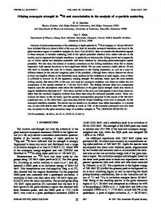
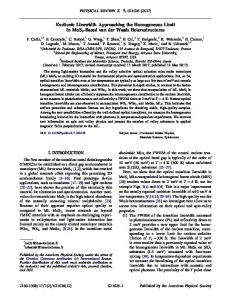
FIG. 1. Real solutions ␥ of Eq. 共3.7兲 with w共k兲 = 1. Below ␾g = 0.537 this equation has no real solutions. Above ␾g two solutions appear, illustrated by the two branches that bifurcate at ␾g. The branch for which ␥ decreases with ␾ 共solid line兲 corresponds to the physical solution of the glass state. In the inset we plot the functional ⌽关␥ ; S兴 as a function of ␥ for the volume fractions ␾ = 0.45, 0.50, 0.55, and 0.60 共from bottom to top兲.

⌬␨*共⬁兲, then this generates a harmonic force term in the effective Langevin equation that describes the Brownian motion of a representative tracer particle 关see Eq. 共B5兲 of Appendix B兴, with a spring constant given by ␨0⌬␨*共⬁兲. From the equipartition theorem, it then follows that 具关⌬x共t兲兴2典 = kBT / 关␨0⌬␨*共⬁兲兴 = ␥. In terms of ␥, Eqs. 共3.1兲 and 共3.2兲 for the nonergodic parameters f共k兲 and f S共k兲 read f共k兲 =

w共k兲␭共k兲S共k兲 w共k兲␭共k兲S共k兲 + k2␥

共3.8兲

␭共k兲 . ␭共k兲 + k2␥

共3.9兲

and f S共k兲 =

These equations clearly show that ␥ and the nonergodic parameters f共k兲 and f S共k兲 only depend on the static structural properties w共k兲, ␭共k兲, and S共k兲, and not on transport properties, such as D0. In Eq. 共3.7兲, ⌽关␥ ; S兴 is a functional of S共k兲 and an ordinary function of ␥. Thus, for a fixed state, i.e., for fixed S共k兲, this equation may be solved by plotting ⌽关␥ ; S兴 as a function of ␥ to see if it crosses unity, and for which value共s兲 of ␥ it does so. This procedure leads to the determination of the real nonzero solutions of Eq. 共3.7兲. This is illustrated in Fig. 1 for the hard-sphere 共HS兲 system, using the static structure factor S共k兲 given by the solution of the Percus-Yevick 共PY兲 approximation 关33,38兴 in the evaluation of the functional ⌽关␥ ; S兴 with w共k兲 = 1 共additive Vineyard-like approximation兲. Let us mention that later on in this paper we shall attempt a quantitative comparison of the theoretical predictions of our dynamical theory with experimental data. At that moment we will compare the additive with the multiplicative approximations, and will replace the

5

10

kσ

15

20

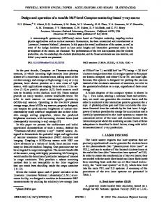
FIG. 2. Nonergodic parameters f共k兲 共heavier solid line兲 and f S共k兲 共lighter solid line兲 calculated with Eqs. 共3.8兲 and 共3.9兲, respectively, with w共k兲 = 1 共additive Vineyard-like approximation兲, for the HS system with S共k兲 given by the PY approximation at the ideal glass transition volume fraction ␾g = 0.537. The dashed lines are the corresponding results for the multiplicative Vineyard-like approximation 关w共k兲 given by Eq. 共3.10兲兴, at its transition volume fraction ␾g = 0.513.

PY by other more accurate approximations for S共k兲. In this section, however, we base our illustrative calculations on the PY approximation, since its analytic solution 关39兴 makes it very easy to program, so that anybody can reproduce the numbers reported here. Of course, the qualitative picture gained will not be affected by these quantitative details. The inset of Fig. 1 exhibits the dependence of the functional ⌽关␥ ; S兴 on ␥ for various volume fractions. Clearly, below a threshold volume fraction ␾g, ⌽关␥ ; S兴 remains below 1 for all ␥, and hence, there are no real solutions. Thus, the system must be in the ergodic state, described by the trivial solution with ⌬␨*共⬁兲 = 0 共i.e., ␥ = ⬁兲. Above ␾g there are two real solutions, one of which corresponds to the glass state. In this manner, we determine this threshold value to be ␾g = 0.537, which is then the prediction of this criterion for the ideal glass transition volume fraction when the PY static inputs are employed. As indicated in Fig. 1, right at the transition there is only a single solution for ␥, namely, ␥ = 1.094⫻ 10−2␴2, where ␴ is the hard-sphere diameter. This solution for ␥ may then be employed in Eqs. 共3.8兲 and 共3.9兲 to determine the nonergodic parameters f共k兲 and f S共k兲; in Fig. 2 these properties are plotted for the HS system at its glass transition volume fraction. For volume fractions beyond the transition, in the glass state, one must choose as the physical solution the branch corresponding to the smallest of the two mathematical nonzero solutions for ␥ 共solid curve in Fig. 1兲. The reason for this is that one can show that ␥ is actually the mean squared displacement of the colloidal particles, as they rattle confined to the frozen cage formed by their neighbors. Since the size of this cage decreases with increasing volume fraction, the mean squared displacement ␥ should decrease as well. The same calculations can be performed for the multiplicative Vineyard-like approximation. Let us mention, however, that in this case the function w共k兲 ⬅ CSEXP共k , z = 0兲 /

041504-6

DYNAMIC ARREST WITHIN THE SELF-CONSISTENT …

PHYSICAL REVIEW E 76, 041504 共2007兲

CSEXP 共k , z = 0兲 contains integrals of derivatives of the pair S potential involved in the second and third short-time moment conditions. These short-time moments do not exist for the hard-sphere potential 共or for other discontinuous interactions兲, due to the divergence of such integrals; this reflects the nonanalytic behavior of F共k , t兲 and its memory function at t = 0 for these potentials 关2,3兴. It happens, however, that the 共k , z = 0兲 above divergent functions CSEXP共k , z = 0兲 and CSEXP S can be evaluated for a soft-sphere potential u共r兲 ⬃ r−␯, and the hard-sphere limit ␯ → ⬁ limit can be taken in the result for their ratio w共k兲. This leads to the finite limit wHS共y兲 = 1 − 3共y 2 sin y + 2y cos y − 2 sin y兲/y 3 , 共3.10兲 with y = k␴. This expression, along with the PY approximation for S共k兲, allows us to apply Eqs. 共3.7兲–共3.9兲 above to the hard-spheres system, with the results ␥ = 1.27⫻ 10−2␴2 and ␾g = 0.513. The corresponding result for the non-ergodic factors are also displayed in Fig. 2. IV. FULL SOLUTION OF THE SELF-CONSISTENT SCHEME

The criterion above constitutes a shortcut to the quick determination of the ergodic-nonergodic transition. An alternative lengthier route is the actual numerical solution of the full self-consistent set of equations in Eqs. 共2.1兲, 共2.2兲, and 共2.5兲–共2.12兲, as illustrated in this section. For this, Eqs. 共2.1兲 and 共2.2兲 are first Laplace inverted, and written as a set of coupled integrodifferential equations involving functions of k and t. These equations, complemented with Eqs. 共2.5兲–共2.12兲, are then discretized in a mesh of points large enough to ensure independence of the solution with respect to the size of the mesh. The discretized system of equations is solved by the method described in Refs. 关40,41兴. Previous to this procedure, one first has to determine the radial distribution function g共r兲 for the desired pair potential, and then calculate the other static properties 关S共k兲, ␹*共k兲, L*0共k兲, ␹*S共k兲, * and L0S 共k兲兴. There is, however, a little technicality to mention, concerning the application of the full self-consistent theory to the hard-sphere system, and has to do with the integrals that * 共k兲. As define the static properties ␹*共k兲, L*0共k兲, ␹*S共k兲, and L0S indicated above, these integrals involve derivatives of the pair potential, which do not exist for the hard-sphere system 共the criterion derived in the previous section does not have this limitation, since it involves only the static structure factor as an input兲. We can circumvent this limitation, however, taking advantage of the principle of dynamic equivalence between soft and hard spheres explained in Ref. 关42兴. Thus, in order to apply the full theory to the HS system, one actually applies it to a soft-sphere system, and a simple rescaling of the results allows us to obtain the properties of the HS system. We have carried out this exercise within the PY approximation for S共k兲 共which, for soft-sphere potentials, has to be solved numerically兲. Proceeding in this manner, at any arbitrary state, we can calculate all the dynamic properties, including F共k , t兲,

FS共k , t兲, and ⌬␨共t兲, and check directly if these properties decay to zero or not, thus leading to the prediction of the location of the glass transition, and of the values of the nonergodic parameters at the transition, and in general, at other glass states. Of course, the results thus obtained turn out to coincide exactly with those of the static criterion above 共Sec. III兲. For example, for the hard-sphere system within the Percus-Yevick approximation this procedure leads, in the case of the additive Vineyard-like approximation, to the location of the glass transition at ␾g = 0.537, and to the same value of the nonergodic parameter ⌬␨*共⬁兲 determined in Sec. III 共␥ = D0 / ⌬␨*共⬁兲 = 1.094⫻ 10−2␴2兲. Finally, the nonergodic parameters f共k兲 and f S共k兲 determined by this exact route agree with those determined in Sec. III 共plotted as the solid curves in Fig. 2兲. Similar comments apply in the case of the multiplicative Vineyard-like approximation. Let us now discuss the relevance of the accuracy of the static structural properties 关S共k兲 and g共r兲兴 employed as inputs in the actual applications of the self-consistent dynamic theory. As indicated before, all the illustrative numerical calculations reported so far have referred to the hard-sphere system, and have involved, for simplicity, the use of the Percus-Yevick approximation for the input static properties S共k兲 and g共r兲. The use of this approximation is itself a source of inaccuracies, which we can minimize or eliminate. For the HS system, we improve the PY approximation with the semiempirical Verlet-Weis 共VW兲 modification 关43兴, which provides virtually exact hard-sphere radial distribution functions up to the freezing transition. The first noticeable consequence of improving the input static properties is a rather dramatic change in the prediction of the location of the ideal glass transition, from ␾g = 0.537 with the PY approximation, to ␾g = 0.563 with the VerletWeis-improved Percus-Yevick 共PY-VW兲 approximation. The mean squared displacement parameter ␥ changes from ␥ = 1.094⫻ 10−2␴2 to ␥ = 1.060⫻ 10−2␴2. The corresponding change in the nonergodic parameters f共k兲 and f S共k兲 turns out to be rather insignificant, and the new results virtually superimpose on the solid lines of Fig. 2. Similar observations apply for the multiplicative Vineyard-like approximation, with ␾g increasing from its PY value ␾g = 0.513 to ␾g = 0.537, and with ␥ decreasing from ␥ = 1.27⫻ 10−2␴2 to ␥ = 1.23⫻ 10−2␴2. From now on in this paper, when referring to the results of our theory for the hard-sphere system, we shall refer to the results obtained with the more accurate PY-VW approximation for the static properties. The numerical solution of the self-consistent theory provides the complete scenario of the relaxation of the dynamics of the system, and of the process of dynamic arrest, as the glass transition is approached. Here we illustrate this process with the theoretical results for the relaxation of the intermediate scattering function described by our theory within the additive approximation in the vicinity of the hard-sphere glass transition. In Fig. 3 we plot the correlator f共k , t兲 ⬅ F共k , t兲 / S共k兲 as a function of time 共in units of t0 ⬅ ␴2 / D0兲 at hard-sphere volume fractions ␾ = 0.559, 0.560, 0.561, 0.562, and 0.563共=␾g兲, with the input static properties provided by the PY-VW approximation. In reality, the short-time dynamics of our theory requires static information that is not de-

041504-7

PHYSICAL REVIEW E 76, 041504 共2007兲

YEOMANS-REYNA et al. 1

0.8

0.8

0.6

0.6

f(kσ)

f(kmaxσ,t/t0)

1

0.4

0.4

0.2

0.2

0 0 10

1

10

2

10

t/t0

0 0

3

10

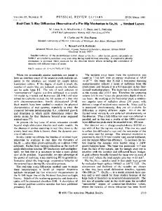
FIG. 3. Time-relaxation of the collective correlator f共k , t兲 ⬅ F共k , t兲 / S共k兲 for the HS system in the vicinity of the glass transition, for the hard-sphere volume fractions 共from bottom to top兲 ␾ = 0.559, 0.560, 0.561, 0.562, and 0.563共=␾g兲. The time is expressed in units of t0 ⬅ ␴2 / D0.

fined for the hard-sphere potential. As explained in detail in Ref. 关42兴, however, the hard-sphere static and dynamic properties can be calculated for a dynamically equivalent softsphere system. Thus, our dynamic calculations for the HS system were in fact performed on a soft-sphere system with pair potential given, in units of the thermal energy kBT = ␤−1, by

␤us共r兲 =

1 2 + 1, 2␯ − 共r/␴s兲 共r/␴s兲␯

共4.1兲

for 0 ⬍ r ⬍ ␴s, and such that it vanishes for r ⬎ ␴s. The static input S共k兲 for this system with ␯ = 100 was provided by the method explained by Verlet and Weis 关43兴, based of the solution of the Percus-Yevick approximation 关38,39兴. Thus, the curves in Fig. 3, corresponding to the sequence of hardsphere volume fractions given above, also correspond to the 共␯ = 100兲 soft-sphere volume fractions ␾共s兲 = 0.571, 0.572, 0.573, 0.574, and 0.575共=␾共s兲 g 兲, respectively. These two sets of volume fractions are related to each other through a simple rescaling, as explained in Ref. 关42兴. V. COMPARISON WITH EXPERIMENTAL DATA

Of course, the systematic and extensive comparison of the present theoretical predictions with the corresponding experimental or computer-simulated data is needed, and will be the subject of separate communications. Here, however, we present a selection of illustrative results, restricted to the analysis of the collective nonergodic parameter f共k兲, for two systems for which experimental data are available, namely, the hard-sphere suspension and a suspension of highly charged particles at low ionic strength. We first discuss the results for the hard-sphere system. The first noticeable theoretical prediction is the location of the ideal glass transition. The transition volume fraction predicted by our theory within the additive Vineyard-like ap-

experiment (φg=0.563) additive (φg=0.563) multiplicative (φg=0.563) multiplicative (φg=0.537)

5

10

kσ

15

20

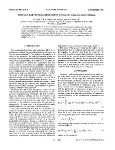
FIG. 4. Nonergodic parameter f共k兲 calculated with Eqs. 共3.7兲 and 共3.8兲 within the additive 共solid line兲 and the multiplicative 共dashed lines兲 Vineyard-like approximations, for the HS system with S共k兲 given by the PY-VW approximation, at the ideal glass transition volume fraction 共solid and heavy lines for ␾g = 0.563, light dashed line for ␾g = 0.537兲. The circles are the experimental data of Ref. 关19兴, measured at ␾g = 0.563.

proximation, ␾g = 0.563, turns out to be in excellent agreement with the experimental results reported in Ref. 关19兴. At this volume fraction we found ␥ = 1.060⫻ 10−2␴. This leads to a ratio ␦ ⬅ 冑具关⌬x共t兲兴2典 / d of the localization length 冑具关⌬x共t兲兴2典 = ␥1/2 to the mean interparticle distance d ⬅ n−1/3 of 0.105, strongly reminiscent of the Lindemann criterion of melting 关46兴. In contrast, the multiplicative Vineyard-like approximation leads to ␾g = 0.537, sensibly smaller than the experimental value, and to a value of the Lindemann ratio of ␦ = 0.112. The other important property that we can compare to experimental data is the collective nonergodic parameter f共k兲. In Fig. 4 we compare the theoretical results for f共k兲 obtained from Eqs. 共3.8兲 and 共3.7兲 within the additive Vineyard-like approximation 共solid line; input static properties provided by the PY-VW approximation兲 at the volume fraction ␾g = 0.563, with the corresponding experimental data, also reported at ␾g = 0.563 关19兴. As we can see, the comparison is very good concerning the height and position of the first maximum of f共k兲. We mention that the position of this maximum of f共k兲 also coincides with the position of the main peak of the static structure factor 共not shown in Fig. 4兲. We observe, however, that at smaller and larger wave vectors, the agreement between theory and experiment for f共k兲 deteriorates appreciably. On the other hand, in Fig. 4 we also plot the theoretical results obtained with the multiplicative Vineyard-like approximation 共dashed lines兲, also using the PY-VW static structure factor S共k兲. In one case 共heavy dashed line兲, we employed the same input S共k兲 as in the additive approximation 共solid line兲, i.e., the PY-VW S共k兲 at the actual experimental volume fraction ␾g = 0.563. The light dashed line was obtained employing the PY-VW S共k兲 at ␾g = 0.537, which is the transition volume fraction predicted by the multiplicative approximation; thus, it corresponds to a zero separation pa-

041504-8

PHYSICAL REVIEW E 76, 041504 共2007兲

5

1

4

0.8

3

0.6

f(kσ)

S(kσ)

DYNAMIC ARREST WITHIN THE SELF-CONSISTENT …

2

0.4

1

0.2

0 2

3

4

5

6

kσ

7

8

9

0 0

10

(a)

experiment additive multiplicative 2

4

6

kσ

8

10

12

14

(b)

FIG. 5. 共a兲 Static structure factor calculated with the PY-VW approximation 共solid curve兲 for the HS system at volume fraction ␾ = 0.58; the symbols correspond to the experimental data of Ref. 关22兴. 共b兲 Theoretical predictions for the nonergodic parameter f共k兲 of a HS suspension at ␾ = 0.58 within the additive 共solid line兲 and multiplicative 共dashed line兲 Vineyard-like approximations; symbols correspond to experimental data reported in Ref. 关22兴.

rameter ␩ ⬅ 共␾ − ␾g兲 / ␾g from the transition volume fraction ␾g = 0.537 predicted by this approximation. Clearly, the latter curve lies far below the experimental data, whereas the other two curves, in which the S共k兲 at the experimentally determined volume fraction ␾g = 0.563 was employed, lie closer to the experimental data for f共k兲. The latter calculation within the multiplicative approximation seems to have a similar degree of accuracy as the additive approximation with the same static input, although it overestimates the height of the main peak of f共k兲. We must bear in mind, however, that these theoretical results of the multiplicative approximation correspond to a separation distance ␩ = 0.05. The results of the additive approximation, on the other hand, correspond to a null separation parameter, thus agreeing with the experimental data in this regard. Let us also notice an important qualitative difference between the additive and the multiplicative approximations, namely, their predictions for the longwavelength limit of f共k兲. As it was quite apparent already from the illustrative results in Fig. 2, the additive approximation leads to the limit limk→0 f共k兲 = 1, whereas the multiplicative approximation leads to limk→0 f共k兲 ⬍ 1. The meaning and relevance of this issue will be discussed below. The nonergodic parameters can also be measured and calculated at volume fractions larger than ␾g, i.e., well inside the glass region. For example, Ref. 关22兴 reports experimental data for the static structure factor and the nonergodic parameter of a hard-sphere system at a volume fraction ␾ = 0.58. Figure 5共a兲 shows the static structure factor calculated from the PY-VW approximation for this volume fraction; the experimental data of Ref. 关22兴 are also included as a reference. This S共k兲 was employed as the input of the dynamic theory in the calculation of the nonergodic parameter f共k兲, and Fig. 5共b兲 illustrates the comparison of our theoretical predictions within both, the additive and the multiplicative approximations, with the corresponding experimental data. We find a similar scenario as observed in Fig. 4, except that now both theoretical predictions coincide in the height of the maxi-

mum of the nonergodic parameter, which is located at the position as the main peak of S共k兲, whereas the position of the experimental first maximum of f共k兲 is shifted to slightly larger wave vectors. Let us finally illustrate the applicability of our theory to an additional system, this time representative of a colloidal system with softer interactions. We refer to a colloidal dispersion of charged particles, also reported in Ref. 关22兴, whose effective pair potential may be modeled by the repulsive screened Coulomb potential,

␤u共r兲 =

冦

K

exp关− z共r/␴ − 1兲兴 , r ⬎ ␴; 共r/␴兲

⬁,

r ⬍ ␴.

冧

共5.1兲

This corresponds to the electrostatic contribution of the wellknown Derjaguin-Landau-Verwey-Overbeek 共DLVO兲 potential 关44,45兴, in which the interaction parameters z and K are, respectively, the inverse Debye screening length 共in units of ␴兲, and the intensity of the pair potential at hard-sphere contact 共in units of kBT兲. Experimental data for this system are also reported in Ref. 关22兴. For one of the samples, the hardsphere diameter and the volume fraction ␾ are experimentally determined to be ␴ = 272 nm and ␾ = 0.27, and data are provided for the static structure factor. In order to use these data as the static input in the dynamic theory, we need to have a smooth representation of the experimental data for S共k兲, and hence, we had to fit these data. For this we used, as a fitting device, the static structure factor calculated within the hypernetted chain 共HNC兲 approximation 关33兴 for the potential above, and the solid line in Fig. 6共a兲 corresponds to the best fit, with z = 3.1587 and K = 11.6555. This fit was actually made not by varying z and K independently, but by using the expressions for these parameters in terms of the charge Q = Ze− of the particles provided by the DLVO model 关3,45兴, namely, z = 冑24␾ZlB / ␴ and K = lBZ2 / 关␴共1 + z / 2兲2兴,

041504-9

PHYSICAL REVIEW E 76, 041504 共2007兲

YEOMANS-REYNA et al. 7

1 1

6 0.8 5 4

f(kσ)

S(kσ)

0.5

3

0.6

0.4

0

2

4

6

8

2 0.2 1 0 2

3

4

5

kσ

6

7

0 0

8

(a)

5

10

kσ

15

20

25

(b)

FIG. 6. 共a兲 Static structure factor calculated with the HNC approximation, and 共b兲 theoretical predictions for the nonergodic parameter f共k兲 for the charged sphere system, with pairwise forces given by Eq. 共5.1兲 at ␾ = 0.27, z = 3.1587, and K = 11.6555; symbols correspond to experimental data in Ref. 关22兴, solid and dashed lines correspond to the additive and multiplicative Vineyard-like approximations, respectively. The inset in 共b兲 enlarges the region where experimental data for f共k兲 are available.

where lB = 共e−兲2 / ⑀kBT is the Bjerrum length, and ⑀ the dielectric constant of the solvent. Next, we employed this S共k兲 as the static input of the dynamic theory to calculate the nonergodic parameters, according to the general results in Sec. III. For this, we first calculated the mean squared displacement ␥ as the solution of Eq. 共3.7兲, with the result ␥ = 2.85⫻ 10−3␴2 for the additive approximation, and ␥ = 8.68⫻ 10−3␴2 for the multiplicative approximation. The corresponding results for f共k兲 are compared with the experimental data in Fig. 6共b兲. As we can see from this comparison, the agreement with the experimental data for the nonergodic parameter f共k兲 of our theoretical predictions within the additive approximation turns out to be very good for all the wave vectors reported in the experiment, whereas the predictions of the multiplicative version turn out to be quantitatively less accurate. VI. ADDITIVE VS MULTIPLICATIVE VINEYARD-LIKE APPROXIMATIONS

There is a number of issues regarding the advantages and limitations of the present SCGLE theory as a proposal of a competitive quantitative theory of dynamic arrest. Its detailed discussion falls outside the scope of the present introductory paper. Let us highlight, however, one particular salient feature, namely, the behavior of the nonergodic parameters in the small wave-vector limit predicted by Eqs. 共3.8兲 and 共3.9兲. Let us first notice that these two equations correctly predict that both f共k兲 and f S共k兲 are smaller than unity for all finite wave-vectors k, as expected from general considerations 关14兴. From Eq. 共3.9兲, however, we have that limk→0 f S共k兲 = 1, and this holds for both the additive and the multiplicative approximations. On the other hand, Eq. 共3.8兲 indicates that the collective nonergodic parameter f共k兲 does depend explicitly on w共k兲, and hence, these two versions of the SCGLE theory will differ in their predictions for f共k兲, as illustrated in the previous section. Although both versions

correctly predict that f共k兲 ⬍ 1 for k ⫽ 0, their longwavelength description of f共k兲 is qualitatively different. Thus, while the additive approximation predicts that limk→0 f共k兲 = 1, the multiplicative approximation predicts that limk→0 f共k兲 ⬍ 1; the latter can be seen by noticing that in general the function w共k兲 ⬅ CSEXP共k , z = 0兲 / CSEXP 共k , z = 0兲 S vanishes as k2 for small k. This contrast between the additive and the multiplicative approximations is clearly apparent in Figs. 4–6. Unfortunately nobody has rigorously derived any form of “sum rule” that fixes the exact value of f共0兲. Let us mention that MCT predicts that f S共0兲 = 1 and that f共0兲 ⬍ 1 关14兴, just the same as the multiplicative version of our SCGLE theory. The value f共0兲 = 1 obtained from the additive SCGLE theory, on the other hand, represents an interesting physical concept, namely, that of a macroscopically infinitely rigid solid. The mechanical rigidity of a system can be described by its mechanical susceptibility ˜␹共k兲, which can be written as ˜␹共k兲 = 关1 − f共k兲兴␹T共k兲, where ␹T共k兲 is its thermodynamic susceptibility 关proportional to S共k兲兴 关33,34兴. A fluid 关f共k兲 = 0兴 may have zero mechanical susceptibility only when ␹T共k兲 vanishes; this would be the case of an incompressible fluid. In a glass, the condition f共k兲 ⬇ 1 is referred to as the stiff glass approximation 关48兴. In this approximation, the glass is stiff 兵˜␹共k兲 = 关1 − f共k兲兴␹T共k兲 ⬇ 0其 because it is a rigid solid 兵关1 − f共k兲兴 ⬇ 0其, and not because it is incompressible 关␹T共k兲 ⬇ 0兴. We may have this condition to apply exactly only at k = 0 关f共0兲 = 1 but f共k兲 ⬍ 1 for k ⫽ 0兴, and this defines an ideally stiff glass only at long wavelengths. Of course, such a condition is not met exactly by real systems 关just as no real system behaves exactly as an ideal gas or as a hardsphere fluid兴, but it defines a distinct and conceptually important reference state. The issue of how relevant this reference state may be to specific real systems must, of course, be submitted to experimental test 关bearing in mind, in analyzing data pertaining to atomic glasses 关49,50兴, possible fundamental differences between colloidal 共strongly overdamped兲 and atomic 共solvent-free兲 systems兴.

041504-10

DYNAMIC ARREST WITHIN THE SELF-CONSISTENT …

PHYSICAL REVIEW E 76, 041504 共2007兲

This issue is, of course, intimately related with our need to discriminate between the additive and the multiplicative approximations, concerning their qualitative, quantitative, and practical usefulness to describe the transition to dynamically arrested states. Nevertheless, in order to check the practical relevance of these qualitative differences between the additive and the multiplicative approximations, the predictions of the self-consistent theory, complemented in one case with the multiplicative and in the other with the additive Vineyard-like approximation, have been compared with the results of Brownian dynamics simulations for specific model systems 关9兴. From such comparisons, it was concluded that the difference of the predictions of both versions of the SCGLE theory are not quantitatively relevant, even in the regimes where these short-time conditions might be most important. The issues just discussed do not provide a definitive criterion for discriminating between the additive and the multiplicative approximations. Thus, we must turn to the comparison of their specific predictions with the corresponding experimental measurements, as a more reliable criterion to prefer one or the other. Although the comparisons presented in the previous section must be complemented with additional similar tests, it seems to us pretty apparent that the additive SCGLE theory provides systematically better agreement with experiment. In addition, it provides a simpler description of the asymptotic long-time singular behavior, typical of the approach to dynamically arrested states. A practical bonus is that it also provides a considerable simplification of the application of the theory to the problem of locating the glass transition, since the corresponding criterion, namely, Eq. 共3.7兲, only involves the static structure factor and not other static properties associated with the short-time moment conditions. For these reasons, and because the quantitative predictions are close enough to the experimental data to allow a direct comparison without the need of adjustable parameters or any form of rescaling of the volume fraction, we propose to adopt the additive Vineyard-like approximation in the SCGLE theory presented in this paper in future applications. VII. SUMMARY AND DISCUSSION

In summary, in this paper we have introduced the selfconsistent generalized Langevin equation theory of colloid dynamics as a practicable approach to the description of the phenomena of dynamic arrest in monodisperse colloidal systems. For this, we provided a summary of the main arguments, derivations, and approximations that serve as the basis in the construction of this self-consistent theory. We then focused on the problem of locating the boundary between the ergodic and nonergodic regions, and discussed an approach to achieve this, derived from the same self-consistent theory. This criterion, which in the MCT literature is referred to as the bifurcation equation, describes the condition needed to restore the ergodicity of the system when it approaches the fluid-glass boundary from the glass side. It consists of an equation for the nonergodic parameter, and the borderline condition is the failure of this equation to have nonzero so-

lutions. This criterion only requires as an input the static structure factor of the system 共which only depends on the interparticle interactions兲, and provides a shortcut to the goal of determining the fluid-glass boundary, alternative to the solution of the self-consistent set of equations describing the full time- and wave-vector-dependence of all the dynamic properties of the system. One of the elements of the SCGLE theory, namely, the Vineyard-like connection between collective and selfdynamics, was the subject of special attention. We considered two versions of this connection, referred to as the additive and the multiplicative Vineyard-like approximations. Although at the end we endorse the former as the most accurate and useful one, we presented and contrasted the results of both approximations in their comparison with the experimental data. Before that, however, and as an illustration and initial calibration, we applied our theory to the hardsphere system, first within the Percus-Yevick approximation for its static properties, yielding ␾g = 0.537, and then with the virtually exact Verlet-Weis-Percus-Yevick S共k兲 共from now on, we only refer to the results of the additive approximation兲. In this manner we arrived at our prediction for the location of the glass transition of the hard-sphere system, ␾g = 0.563, which is about the best quantitative theoretical estimate of the location of the glass transition of the hardsphere system. The comparison of the predicted nonergodic parameters at, and above, this glass transition volume fraction, with the corresponding experimental data, was presented in Figs. 4 and 5, respectively. These comparisons indicate that, for the volume fraction corresponding to ␾g, the agreement of the theory with the experimental data is very good regarding the height and position of f共k兲 at its first maximum. A similar scenario was observed at the larger volume fraction, ␾ = 0.58, except that now we observe that the theoretical predictions place the maximum of f共k兲 at the same position of the main peak of S共k兲, whereas the experimental data for f共k兲 exhibits this first maximum at slightly larger wave vectors. In contrast, the comparison in Fig. 6共b兲 with the experimental data of Ref. 关22兴 for the nonergodic parameter of the dispersion of charged particles exhibits a remarkable qualitative and quantitative agreement. In particular, the position of the first maximum of f共k兲 coincides with the position of the main peak of S共k兲 according to both theory and experiment. We must stress that our theoretical predictions do not involve any sort of adjustable parameters. As indicated in Sec. III, the parameter ␥, solution of Eq. 共3.7兲, is the mean squared displacement 具关⌬x共t兲兴2典 of the colloidal particles in the glass state, as they undergo Brownian motion inside the frozen cage formed by their neighbors. It is then interesting to find out if this quantity has any special value at the glass transition. According to the theoretical prediction for ␥ reported in the previous sections, the hardsphere glass melts when ␥ = 1.060⫻ 10−2␴2, which means that the root mean square displacement is of the order of one tenth of the hard-sphere diameter; notice that at the volume fraction involved, ␾g = 0.563, the mean interparticle distance d ⬅ n−1/3 is d = 0.98␴, so that ␦ = 冑具关⌬x共t兲兴2典 / d ⬇ 0.105. This is strongly reminiscent of the Lindemann criterion for the melting of a crystal 关46兴. A similar calculation for the

041504-11

PHYSICAL REVIEW E 76, 041504 共2007兲

YEOMANS-REYNA et al.

and of FAI-UASLP. The authors are deeply indebted to Professor J. Bergenholtz, Professor A. Banchio, and Professor G. Nägele for useful discussions. We are also particularly grateful to one of the anonymous referees for his and/or her exceptionally careful and critical reading of our manuscript.

charged sphere suspension leads to similar conclusions. In fact, we find more generally that our theory predicts a very distinctive and universal Lindemann-like criterion for the melting of a glass for systems with repulsive 共soft or hard兲 interactions. This, and many other issues related to the description of dynamic arrest in monodisperse suspensions, can be addressed with the present theory, which may also be extended to consider more complex and interesting situations. These issues, however, will be discussed in detail in future communications.

APPENDIX A: STATIC PROPERTIES

For immediate reference, in this appendix we quote the * 共k兲, ␹*S共k兲, and expressions for the static properties ␹*共k兲, L0S * L0S共k兲 associated to F共k , z兲 and FS共k , z兲 关see Eqs. 共2.3兲 and 共2.4兲兴 in terms of the two- and three-particle correlation functions, g共r兲 and g共3兲共r , r⬘兲. For the details of their derivation, we refer the reader to the original source, namely, Ref. 关6兴. These expressions are

ACKNOWLEDGMENTS

This work was supported by the Consejo Nacional de Ciencia y Tecnología 共CONACYT, México兲, through Grants No. SEP-2004-C01-47611 and No. SEP-2003-C02-44744,

␹*共k兲 = 1 + n

L*0共k兲 = nD0

冕

d3rg共r兲

+

2D0n k

+

D 0n 2 k2

冕 冕

冕

d3rg共r兲

冉

⳵2␤u共r兲 D 0n 2 2 关1 + 2 cos kz兴 − ⳵z k2

d3rg共r兲

冊

1 ⳵2␤u共r兲 1 − cos共kz兲 , − 2 2 ⳵z k S共k兲

2D0n ⳵3␤u共r兲 sin kz + 2 ⳵z3 k

冕

冋冕

d3rg共r兲

冋冕

1 n k2

册 冋 册 冋 册冋

⳵2␤u共r兲 共1 − cos kz兲 ⳵z2

d3rg共r兲共1 − cos kz兲

d3rd3r⬘g共3兲共r,r⬘兲共1 − 2 cos kz + cos关k共z − z⬘兲兴兲 ⫻

␹*S共k兲 =

d3rg共r兲

共A1兲

⳵ ⵱ ␤u共r兲 ⳵z

2

2

册

⳵ ⵱ ␤u共r兲 ⳵⵱⬘␤u共r⬘兲 · , ⳵z ⳵z⬘

共A2兲

册

⳵2␤u共r兲 , ⳵z2

共A3兲

and

冋冕

* 共k兲 = k2D0 n k2L0S

+ D 0n 2

冕

d3rg共r兲

册 冋冕 冋 册冋

⳵2␤u共r兲 − D 0n 2 ⳵z2

d3rd3r⬘g共3兲共r,r⬘兲

d3rg共r兲

册 册

⳵2␤u共r兲 ⳵z2

2

+ 2D0n

冕

d3rg共r兲

冋

⳵ ⵜ ␤u共r兲 ⳵z

册

2

⳵ⵜ⬘␤u共r⬘兲 ⳵ ⵜ ␤u共r兲 · . ⳵z ⳵z⬘

共A4兲

In the equations above, u共r兲 is the effective interaction pair potential between colloidal particles. Finally, we should mention that in this paper we have systematically dropped the subindex “UU” employed in Ref. 关6兴, where 共kBT / M兲2 times ␹*共k兲, ␹*S共k兲, 共S兲 共S兲 * 共k兲 are denoted, respectively, by ␹UU共k兲, ␹UU 共k兲, LUU共k兲, and LUU 共k兲. L*0共k兲, and L0S The integrals involving g共3兲共r , r⬘兲 in these equations were evaluated in practice with the use of Kirkwood’s superposition approximation, g共3兲共r , r⬘兲 ⬇ g共r兲g共r⬘兲g共兩r − r⬘ 兩 兲, plus the additional simplification of approximating g共兩r − r⬘ 兩 兲 by its asymptotic value of 1. This leads, in particular, to replacing the integral in the last term of Eq. 共A2兲, ⌬m共3兲共k兲 ⬅

冕

d3rd3r⬘g共3兲共r,r⬘兲„1 − 2 cos共k · r兲 + cos兵关k · 共r − r⬘兲兴其… ⫻ 共k · ⵱兲共k · ⵱⬘兲共⵱ · ⵱⬘兲␤u共r兲␤u共r⬘兲,

共A5兲

by ⌬m共3兲共k兲 =

冋冕

d3rg共r兲关1 − cos共k · r兲兴共k · ⵱兲 ⵱ ␤u共r兲 041504-12

册

2

.

共A6兲

DYNAMIC ARREST WITHIN THE SELF-CONSISTENT …

PHYSICAL REVIEW E 76, 041504 共2007兲

The corresponding approximate expression for the case of self-diffusion is identical, but without the term involving cos共k · r兲. Thus, within these approximations, the only static input needed by the SCGLE theory is g共r兲. APPENDIX B: DERIVATION OF EQ. (2.11)

This appendix summarizes the derivation of Eq. 共2.11兲 provided in detail in Ref. 关10兴. Consider a monodisperse colloidal suspension formed by N spherical particles in a volume V in the absence of hydrodynamic interactions, whose microscopic dynamics is described by the N-particle Langevin equations 关1–3兴 M

dvi共t兲 = − ␨ovi共t兲 + fi共t兲 + 兺 Fij共t兲, dt j⫽i

i = 1,2, . . . ,N. 共B1兲

In these equations, M is the mass, vi共t兲 is the velocity, and ␨o is the free-diffusion friction coefficient, of the ith particle. Also, fi共t兲 is a Gaussian white random force of zero mean, and variance 具fi共t兲f j共0兲典 = kBT␨o2␦共t兲␦ij JI 共i , j = 1 , 2 , . . . , N ; JI being the 3 ⫻ 3 unit tensor兲. The pairwise force that the jth particle exerts on particle i is given by Fij = −ⵜiu共兩ri − r j 兩 兲. If one is only interested in the motion of individual tracer particles, then Eq. 共B1兲 for one specific particle 共denoted by the index i = T兲 may be rewritten exactly as M

dvT共t兲 = − ␨TovT共t兲 + fT共t兲 + dt

冕

in the presence of the “external” field produced by, and described from a reference frame fixed to, the tracer particle. Thus, we need a relaxation equation that couples the timederivative of the variable ␦n*共r , t兲 with itself and with vT共t兲. Its most general structure is dictated by the general principles of linear irreversible thermodynamics 关11兴 to be a linear version of a generalized diffusion equation, with the following general structure 关10兴:

⳵␦n*共r,t兲 = 关ⵜneq共r兲兴 · vT共t兲 − dt

冕

M

dvT共t兲 = − ␨TovT共t兲 + fT共t兲 − dt

The variable ␦n 共r , t兲 represents the fluctuations around equilibrium of the local concentration of colloidal particles

t

dt⬘⌬J ␨共t − t⬘兲 · vT共t⬘兲 + F共t兲,

0

where the new fluctuating force F共t兲 is related with the time␨共t兲 through 具F共t兲F共0兲典 dependent friction tensor ⌬J J J = Mk T⌬␨共t兲, with ⌬␨共t兲 given by the following exact result: ⌬J ␨共t兲 = −

共B3兲 *

冕

共B5兲

B

d3r关ⵜu共r兲兴␦n*共r,t兲.

共B4兲

where the first term on the right-hand side is a linearized streaming term and f共r , t兲 is a fluctuating term, related to D*共r , r⬘ ; t兲 by 兰d3r⬙具f共r , t兲f共r⬙ , t⬘兲典␴共r⬙ , r⬘兲 = D*共r , r⬘ ; t − t⬘兲, with ␴共r , r⬘兲 ⬅ 具␦n*共r , 0兲␦n*共r⬘ , 0兲典. Formally solving Eq. 共B4兲 and substituting the solution for ␦n*共r , t兲 in Eq. 共B3兲 leads to

共B2兲

dvT共t兲 = − ␨TovT共t兲 + fT共t兲 + dt

d3r⬘D*共r,r⬘ ;t − t⬘兲

0

⫻␦n 共r⬘,t⬘兲 + f共r,t兲,

冕 冕 d 3r

d3r⬘关⵱u共r兲兴␹*共r,r⬘ ;t兲关⵱⬘neq共r⬘兲兴, 共B6兲

*

M

dt

*

d3r关⵱u共r兲兴n*共r,t兲,

where n 共r , t兲 is the local concentration of the other colloidal particles at time t and position r 关referred to the position xT共t兲 of the tracer particle兴. In other words, n*共r , t兲 is defined as n*共r , t兲 ⬅ n关xT共t兲 + r , t兴, with n共x , t兲 ⬅ 兺i⫽T␦关x − xi共t兲兴 being the local concentration at time t and position x, the positions xi共t兲 and x being referred to the laboratory reference frame. An important observation is then that the direct interactions between the particles, represented by the pairwise potential u共r兲, couple exactly the motion of the tracer particle with the motion of the other particles only through the collective variable n*共r , t兲. The equilibrium average neq共r兲 of n*共r , t兲 is given by neq共r兲 = ng共r兲, with n being the number concentration, and g共r兲 the radial distribution function of the bulk suspension. Due to the radial symmetry of the force 关−⵱u共r兲兴 and of neq共r兲, the integral in Eq. 共B2兲, evaluated at n*共r , t兲 = neq共r兲, vanishes. Thus, Eq. 共B2兲 is a linear equation coupling exactly the time derivative of the tracer’s velocity vT共t兲 with itself and with the variable ␦n*共r , t兲 ⬅ n*共r , t兲 − neq共r兲, namely,

冕 ⬘冕 t

where ␹*共r , r⬘ ; t兲 is the propagator, or Green’s function, of the diffusion equation in Eq. 共B4兲, i.e., it solves the equation

⳵␹*共r,r⬘ ;t兲 =− dt

冕 ⬘冕 t

dt

d3r⬙D*共r,r⬙ ;t − t⬘兲␹*共r⬙,r⬘ ;t⬘兲,

0

共B7兲 with initial value ␹*共r , r⬘ ; t = 0兲 = ␦共r − r⬘兲. Notice that, since the initial value ␦n*共r , t = 0兲 is statistically independent of vT共t兲 and f共r , t兲, the density-density time-correlation function G*共r , r⬘ ; t兲 ⬅ 具␦n*共r , t兲␦n*共r⬘ , 0兲典, which is the van Hove function of the particles surrounding the tracer particle, and observed from the tracer particle’s reference frame, is also a solution of the same equation with initial value G*共r , r⬘ ; t = 0兲 = ␴共r , r⬘兲. To simplify the notation, let us rewrite Eq. 共B6兲 as J where the convolution ⌬␨共t兲 = −关ⵜu†兴 ⴰ ␹*共t兲 ⴰ 关ⵜneq兴, 兰d3r⬙F共r , r⬙兲G共r⬙ , r⬘兲 between two arbitrary functions F and G is written as the matrix product F ⴰ G, and similarly with the “共column兲 vectors” u and neq. In this notation, the dagger means transpose. With this notation, let us recall an additional exact relation between the “vectors” u, neq, and the “matrix” ␴. This is the so-called Wertheim-Lovett relation 关10,47兴, 关ⵜneq兴 = −␤␴ ⴰ 关ⵜu兴, of the equilibrium theory of inhomogeneous fluids. This relation, along with the definition of the inverse matrix ␴−1, 关␴−1␴ = I, with I being the unit

041504-13

PHYSICAL REVIEW E 76, 041504 共2007兲

YEOMANS-REYNA et al.

matrix, I共r , r⬘兲 ⬅ ␦共r − r⬘兲, where ␦ is Kronecker’s ⌬ function兴, allows us to write Eq. 共B6兲 in a variety of different but equivalent and exact manners. In particular, we will employ the following:

where we have used the fact that the van Hove function G*共t兲 can be written as G*共t兲 = ␹*共t兲␴. This is the exact result for ⌬J ␨共t兲 that leads to the general but approximate expression in Eq. 共2.11兲. The approximations required are related to the general properties of the functions G*共r , r⬘ ; t兲 and ␴共r , r⬘兲. The latter is just the twoparticle distribution function of the colloidal particles surrounding the tracer particle, but subjected to the “external” field u共r兲 exerted by this tracer particle. Thus, it is effectively a three-particle correlation function. Only if one ignores the effects of such an “external” field, one can write ␴共r , r⬘兲 = ␴共兩r − r⬘兩兲 ⬅ n␦共r − r⬘兲 + n2关g共兩r − r⬘兩兲 − 1兴. Similarly, we may also approximate G*共r , r⬘ ; t兲 by G*共兩r − r⬘兩 ; t兲.

This is referred to as the “homogeneous fluid approximation” 关10兴, which allows us to write G*共r , r⬘ ; t兲 = 共1 / 2␲兲3 兰 d3k exp关ik · r兴F*共k , t兲, with F*共k , t兲 ⬅ 具兺Ni,j exp兵ik · 关ri共t兲 − r j共0兲兴其典. The latter is the intermediate scattering function, except for the asterisk indicating that the position vectors ri共t兲 and r j共0兲 have the origin in the center of the tracer particle. Denoting by xT共t兲 the position of the tracer particle referred to a laboratory-fixed reference frame, we may rewrite F*共k , t兲 ⬅ 具(exp兵ik · 关xT共t兲 N − xT共0兲兴其) · (兺i,j exp兵ik · 关xi共t兲 − x j共0兲兴其)典, where ri共t兲 is the position of the ith particle in the fixed reference frame. Approximating the average of the product in this expression by the product of the averages, leads to F*共k , t兲 = F共k , t兲FS共k , t兲, which we refer to as the decoupling approximation 关10兴. The result in Eq. 共2.11兲 is obtained from the exact result in Eq. 共B8兲 above, plus the introduction of the two approximations ␨共t兲 must just described. For spherical particles, the tensor ⌬J J J be diagonal, ⌬␨共t兲 = ⌬␨共t兲 I, and Eq. 共2.11兲 refers to the scalar function ⌬␨共t兲.

关1兴 P. N. Pusey, in Liquids, Freezing and the Glass Transition, edited by J. P. Hansen, D. Levesque, and J. Zinn-Justin 共Elsevier, Amsterdam, 1991兲. 关2兴 W. Hess and R. Klein, Adv. Phys. 32, 173 共1983兲. 关3兴 G. Nägele, Phys. Rep. 272, 215 共1996兲. 关4兴 L. Yeomans-Reyna and M. Medina-Noyola, Phys. Rev. E 64, 066114 共2001兲. 关5兴 L. Yeomans-Reyna, H. Acuña-Campa, and M. Medina-Noyola, Phys. Rev. E 62, 3395 共2000兲. 关6兴 L. Yeomans-Reyna and M. Medina-Noyola, Phys. Rev. E 62, 3382 共2000兲. 关7兴 L. Yeomans-Reyna, H. Acuña-Campa, F. de Jesus GuevaraRodríguez, and M. Medina-Noyola, Phys. Rev. E 67, 021108 共2003兲. 关8兴 M. A. Chávez-Rojo and M. Medina-Noyola, Physica A 366, 55 共2006兲. 关9兴 M. A. Chávez-Rojo and M. Medina-Noyola, Phys. Rev. E 72, 031107 共2005兲. 关10兴 M. Medina-Noyola, Faraday Discuss. Chem. Soc. 83, 21 共1987兲. 关11兴 M. Medina-Noyola and J. L. del Río-Correa, Physica A 146, 483 共1987兲. 关12兴 C. A. Angell, Science 267, 1924 共1995兲. 关13兴 P. G. Debenedetti and F. H. Stillinger, Nature 共London兲 410, 359 共2001兲. 关14兴 W. Götze, in Liquids, Freezing and Glass Transition, edited by J. P. Hansen, D. Levesque, and J. Zinn-Justin 共North-Holland, Amsterdam, 1991兲. 关15兴 W. Götze and L. Sjögren, Rep. Prog. Phys. 55, 241 共1992兲. 关16兴 W. Götze and E. Leutheusser, Phys. Rev. A 11, 2173 共1975兲. 关17兴 W. Götze, E. Leutheusser, and S. Yip, Phys. Rev. A 23, 2634 共1981兲. 关18兴 W. van Megen and P. N. Pusey, Phys. Rev. A 43, 5429 共1991兲. 关19兴 W. van Megen, S. M. Underwood, and P. N. Pusey, Phys. Rev. Lett. 67, 1586 共1991兲.

关20兴 W. van Megen, T. C. Mortensen, S. R. Williams, and J. Müller, Phys. Rev. E 58, 6073 共1998兲. 关21兴 E. Bartsch et al., J. Chem. Phys. 106, 3743 共1997兲. 关22兴 C. Beck, W. Härtl, and R. Hempelmann, J. Chem. Phys. 111, 8209 共1999兲. 关23兴 G. Szamel and H. Löwen, Phys. Rev. A 44, 8215 共1991兲. 关24兴 N. J. Wagner, Phys. Rev. E 49, 376 共1994兲. 关25兴 共a兲 G. Nägele, J. Bergenholtz, and J. K. G. Dhont, J. Chem. Phys. 110, 7037 共1999兲; 共b兲 108, 9893 共1998兲. 关26兴 共a兲 G. Nägele and J. K. G. Dhont, J. Chem. Phys. 108, 9566 共1998兲; 共b兲 G. Nägele and P. Baur, Physica A 245, 297 共1997兲. 关27兴 A. J. Banchio, J. Bergenholtz, and G. Nägele, J. Chem. Phys. 113, 3381 共2000兲. 关28兴 A. J. Banchio, J. Bergenholtz, and G. Nägele, Phys. Rev. Lett. 82, 1792 共1999兲. 关29兴 G. Szamel, Phys. Rev. Lett. 90, 228301 共2003兲. 关30兴 J. Wu and J. Cao, Phys. Rev. Lett. 95, 078301 共2005兲. 关31兴 共a兲 R. Verberg, I. M. de Schepper, and E. G. D. Cohen, Phys. Rev. E 61, 2967 共2000兲; 共b兲 E. G. D. Cohen and I. M. de Schepper, J. Stat. Phys. 63, 242 共1991兲; 共c兲 I. M. de Schepper, E. G. D. Cohen, P. N. Pusey, and H. N. W. Lekkerkerker, J. Phys.: Condens. Matter 1, 6503 共1989兲. 关32兴 B. Cichocki and B. U. Felderhof, Physica A 204, 152 共1994兲. 关33兴 J. P. Hansen and I. R. McDonald, Theory of Simple Liquids 共Academic Press, New York, 1976兲. 关34兴 J. L. Boon and S. Yip, Molecular Hydrodynamics 共Dover Publications, New York, 1980兲. 关35兴 共a兲 J. L. Arauz-Lara and M. Medina-Noyola, Physica A 122, 547 共1983兲; 共b兲 G. Nägele, M. Medina-Noyola, R. Klein, and J. L. Arauz-Lara, ibid. 149, 123 共1988兲. 关36兴 H. Acuña-Campa and M. Medina-Noyola, J. Chem. Phys. 113, 869 共2000兲. 关37兴 G. H. Vineyard, Phys. Rev. 110, 999 共1958兲. 关38兴 J. K. Percus and G. J. Yevick, Phys. Rev. 110, 1 共1957兲. 关39兴 M. S. Wertheim, Phys. Rev. Lett. 10, 321 共1963兲.

␨共t兲 = kBT关ⵜneq†兴 ⴰ ␴−1 ⴰ G*共t兲 ⴰ ␴−1 ⴰ 关ⵜneq兴, ⌬J

共B8兲

041504-14

DYNAMIC ARREST WITHIN THE SELF-CONSISTENT …

PHYSICAL REVIEW E 76, 041504 共2007兲

关40兴 M. Fuchs, W. Götze, I. Hofacker, and A. Latz, J. Phys.: Condens. Matter 3, 5047 共1991兲. 关41兴 A. J. Banchio, Ph.D. thesis, University of Konstanz, 1999. 关42兴 F. de J. Guevara-Rodríguez and M. Medina-Noyola, Phys. Rev. E 68, 011405 共2003兲. 关43兴 L. Verlet and J.-J. Weis, Phys. Rev. A 5, 939 共1972兲. 关44兴 E. J. W. Verwey and J. T. G. Overbeck, Theory of the Stability of Lyophobic Colloids 共Elsevier, Amsterdam, 1948兲. 关45兴 M. Medina-Noyola and D. A. McQuarrie, J. Chem. Phys. 73,

6229 共1980兲. F. A. Lindemann, Phys. Z. 11, 609 共1911兲. R. Evans, Adv. Phys. 28, 143 共1979兲. W. Götze and M. R. Mayr, Phys. Rev. E 61, 587 共2000兲. T. Scopigno, G. Ruocco, F. Sette, and G. Monaco, Science 302, 849 共2003兲. 关50兴 U. Buchenau and A. Wischnewski, Phys. Rev. B 70, 092201 共2004兲.

关46兴 关47兴 关48兴 关49兴

041504-15