Dynamic Associative Memory, Based on Open Recurrent Neural Network Alexander M. Reznik, Dmitry A. Dziuba Abstract—Mathematical model of open dynamic recurrent neural network, that hasn't hidden neurons, is described. Such network has dynamic attractors, that are sequences of transitions between one attractor state to another, according to input signal sequences. Concept of “freezing” of such dynamics with the use of virtual static recurrent network is proposed. Solution of generalized stability equation is used for development of non-iterative method for training dynamic recurrent networks. Estimations of attraction radius and training set size are obtained. Using of the open dynamic recurrent network as dynamic associative memory is studied and possibility of control of dynamic attractors by changing level of influence of different feedback components is shown. Software model of the network was developed, and experimental study of its behavior for reproducing of sequences of distorted vectors was performed. Analogy between dynamic attractors and neural activity patterns, that support hypothesis of local neural ensembles, with structure and functions similar to dynamic recurrent networks in neocortex, is remarked.
I. INTRODUCTION Associative properties of recurrent neural networks, for example, Hopfield network, are based on their multistability [1,2]. Stable states (attractors) of such network may be treated as memorized images, and process of convergence, i.e. consecutive state changes in the direction of closest attractor, – as finding of solution by association to initial image. In dynamic recurrent neural networks with delayed connections, attractors are not stable states, but stable sequences of states, that are responses on external inputs [35]. Such sequences may be treated as dynamic images, and dynamic recurrent network itself – as dynamic associative memory, that is able to recognize and reproduce memorized images. Learning of dynamic recurrent networks usually is performed by iterative error back propagation through time [6-8]. This process requires significant time and is computationally expensive, because formation of recurrent connections often isn't monotonic, and its results aren't always stable. Problems arise also for estimation of training results, because methods and criteria, developed for static networks, aren't always applicable for dynamic ones. Due to this, detailed study of relatively simple open dynamic networks without hidden neurons, so their state can be continuously monitored, is important. Well known Manuscript received December 30, 2008. A. M. Reznik is with the Institute of Mathematical machines & Systems Problems NAS of Ukraine (e-mail: neuro@ immsp.kiev.ua). D. A. Dziuba is with the Institute of Mathematical machines & Systems Problems NAS of Ukraine (e-mail:
[email protected]).
analytical methods and non-iterative learning [9], that doesn't require much computational resources, may be used for them. Clarity of open neural networks makes them promising for modeling elements of neural system, especially associative fields and recurrent visual cortex structures [8]. They may happen to be more efficient than more complicated dynamic networks (for example, dynamic associative memory) in different applied systems. In this article, new model of dynamic associative memory, based on open dynamic recurrent network, is proposed. In part 2, structure and behavior of such network is analyzed, concept of virtual static network, that allows use of noniterative methods, is proposed. Part 3 contains estimation of associative properties of open dynamic recurrent networks. In part 4, using of recurrent network as dynamic associative memory is described. Part 5 contains results of experiments, performed on developed software model of the open dynamic recurrent network, that illustrates dynamic associative memory mechanism. Part 6 contains conclusions, particularly, assumption of existence of similar mechanisms in the lateral neurostructures of the brain. II.OPEN DYNAMIC RECURRENT NEURAL NETWORK We will denote as “open” such network without hidden neurons, where all signals on inputs of all neurons are open for external observation. Examples of this kind of networks are the Hopfield network and bidirectional associative memory [1, 10]. If backward connections of such network have delays, network will have dynamic properties. Fig. 1 illustrates the scheme of an open dynamic recurrent network, that has N 1 neurons, and, correspondingly, N 1 binary outputs. Number of inputs
N 0 may be different
For statical network, this means that neurons outputs (and, correspondingly, postsynaptic potentials) become timeindependent. In the dynamic network, that have delayed recurrent connections, this isn't the goal. Its dynamic attractors are sequences of static attractor states, that are reactions on corresponding sequences of external inputs. m th vector of such sequence is denoted as R *m . It has three
R1,m+ 1 - output values that corresponds to m + 1 -th frame of the dynamic attractor, R1,m− 1 - delayed output, that corresponds to m − 1 -th frame of the attractor, R 0,m - current external stimuli, that corresponds to current m -th frame of the attractor. vector components:
Using this vector in (3'), we will receive that Fig.1 Open dynamic recurrent neural network
R1,m+ 1 = Λ [W 11 R1,m + 1 + W 1τ R1,m− 1 + W 1, 0 R 0,m ], (4)
from the number of neurons, but in this work it is assumed to be equal to N 1 . We assume binary input signals. Amount
N τ may be different from number of neurons ( N τ ≤ N 1 ), but is assumed to be equal to N 1 . Also, we assume that delays length 2τ is the same for one of delayed connections
half of recurrent connections (another half doesn't have any delay). Combination of input and delayed signals, that are simultaneously acting on inputs of all neurons, describes N * -dimensional state vector of neural network:
R1,m+ 1 , R1,m − 1 and R 0,m are known, this equation may be solved for matrices W 11 , W 1τ and W 10 . If vectors
For this, virtual static symmetric network with may be used. State vector components
S 0 (t )
N1 n= 1
,
vector of postsynaptic potentials (PSP):
S 1 (t ) = W 11Z 1 (t ) + W 1τ Z 1 (t − τ ) + W 10 Z 0 (t ) , (2) Z 1 (t ) , Z 1 (t − τ ) - vectors of current and
where:
Z 0 (t ) - input vector;
delayed reactions of neurons; 11
W ,W
1τ
and
W
10
- weight matrices for connections
between outputs and inputs, delayed outputs and inputs, and external stimuli and inputs. In the attractor state the following condition is satisfied:
{
}
Z (t + 1) = F [ S (t )] = f ( s (t ) 1
1
1 n
N1 n= 1
.
(3)
Or, considering that activation function is monotonic:
Z (t + 1) = Λ S (t ) 1
where ( λ ii
1
(3')
Λ is a positive-definite diagonal matrix N 1 × N 1
≥ 0 ).
W 00 Z 0 (t )
= W τ 1Z 1 (t ) + W τ τ Z 1 (t − τ ) + W τ 0 Z 0 (t ) W 01Z 1 (t ) + W 0τ Z 1 (t − τ ) + W 0τ Z 0 (t )
(1)
f (.) is the neuron's activation function; S 1 (t ) –
where:
W 01 W 0τ
W 10 Z 1 (t ) W τ 0 Z 1 (t − τ ) =
W 11Z 1 (t ) + W 1τ Z 1 (t − τ ) + W 1τ Z 0 (t )
current network reaction could be represented as the following vector:
}
Z 1 (t ) , Z 1 (t − τ ) and Z 0 (t ) . PSP of virtual
S 1 (t ) W 11 W 1τ S * (t ) = S 1 (t − τ ) = W τ 1 W τ τ
*
{
Z * (t ) of such network has three
network may be represented by matrix equation: .
Z * (t ) = {zn* }nN= 1 , where N * = N 1 + N τ + N 0 . Using the sequence of states in discrete time points ...t − 1, t , t + 1... ,
Z 1 (t + 1) = F [ S 1 (t )] = f ( s1n (t )
N * neurons
We'll assume that dynamic attractor is a sequence of vectors in discrete time points ...t − τ , t , t + τ ... , and using this representation, correspondence between dynamic network states and its attractors may be determined: ⇨
Z 1 (t )
1 R1,m+ 1 ; Z (t − τ ) ⇨ R1,m− 1 . Sequence of attractor states
may be represented as following matrix:
R1, 2 ... R1,m + 1... R1, M + 1 ℜ * = R1,0 ... R1,m − 1... R1, M − 1 , R 0 ,1... R 0 ,m .... R 0 , M where rows are static attractor vectors of virtual network. By the analogy with (4), generalized equation of attractor state of virtual network may be written as:
ℜ * = Λ W *ℜ * , Solution for
(5)
*
W may be obtained:
W * = Λ − 1ℜ * (ℜ * ) +
,
(6)
(ℜ * ) + - pseudoinverse matrix ℜ * [11]. Vectors R1,m and R 0,m are binary, so we may assume Λ =І. To find elements of W * algorithm of pseudoinversion where
should be used [12,13]: +1 m+ 1 wi*m = wi*m − sim + 1 )(rjm + 1 − s mj + 1 ) d m + 1 ; ,j , j + ( ri
∑
sim+ 1 =
∑
d m+ 1 =
N
*
k= 1 *
(7)
wik*m rkm+ 1 ;
N m+ 1 k = 1 ik
r
(rkm+ 1 − skm+ 1 ) ,
rkm + 1 is the component of the vector R *m+ 1 . W * = ℜ * (ℜ * ) + is a projection matrix in linear space
where
ℑ , that is stretched on М vectors from ℜ * . It has following properties:
W = (W ) ; *
* 2
∑
N*
TrW * =
∑
wi*,i =
wi*,i =
j= 1
( wi*, j ) 2 ; N* i= 1
wi*,i = M ;
M ; N*
M M M M 1 − * ≥ ( wi*, j ) 2 ≥ * * 1− , i ≠ j (8) * N N N ( N − 1) N * Value of nondiagonal elements is between higher estimate, that is made for the case of a low-density matrix, with many close to zero elements, and lower estimate, that is made for the case of almost equal elements values. Diagonal elements determine weights of positive feedback connections. Increase of the
M N * ratio leads to weakening of neural reaction
on external stimuli, convergence failure and to false attractors. In the case of recurrent connections delays absence (τ =0) symmetric network, calculated according to (7), transforms into threshold-controlled associative memory [13], that has M < N 1 / 2 main attractors, presented by pairs of vectors
{R
1, m + 1
, R 0, m
}
M m= 1
. If such network is in unstable state,
convergence process starts, so its states are changing sequentially in the direction of the nearest main attractor. In the case of presence of delayed recurrent connections, matrix W * contains blocks W 11 , W 1τ and W 10 , that corresponds to real connections. In such network convergence process is restricted by the τ steps (after that time, the next frame of the dynamic attractor will come on delayed inputs). This restriction doesn't prevent existence of dynamic attractors, for which any next state satisfies the attractor conditions. Dynamic attractor may start from any
vector from the sequence, presented by matrix
ℜ * , and will
end by its last vector R *,M + 1 . If initial state isn't the attractor state, situation is more complicated, because, unlike monotonic approximation to the nearest attractor in the case of static symmetrical network, behavior of dynamic network in non-attractor state may be not monotonic. III. ATTRACTOR RADIUS OF THE DYNAMIC RECURRENT NETWORK Behavior of a static recurrent network depends on associative memory fill ratio, that is determined by ratio of attractors number to neurons number M N . Convergence process may stop outside of main attractors, and with
M N ratio, possibility of such stop increases. In Hopfield network convergence stops when M N > 0,14 increasing
[1,2,7]. With the use of pseudoinverse algorithm, this ratio is close to 0,25 [14]. The highest ratio M N ≈ 0,7 was achieved when special method of desaturation of weight matrix was used [15]. To estimate attraction properties of a static network, in [12] was proposed the concept of attractor radius, that is defined as number of neurons, that changes their output at the last step of convergence into state of main attractor. This criterion is used for synchronous network state calculation mode, when at first PSP of all neurons is calculated, and then simultaneously all their outputs are changing into new value. In [2] it was shown, that it is efficient also for asynchronous calculation mode. We will try to use this criterion for the dynamic recurrent network. For this, we'll use earlier described model of the virtual static network, and will analyze its behavior at the last step of convergence into the state of main attractor. Let
zj
to be the reaction value of the j-th neuron of the virtual network before transition into attractor state, transition. We'll assume
rj – after
rj = 1 . According to the attractor
state equation
ri =
∑
N* j= 1
wi*, j rj
,
and considering that during the transition into attractor state signs of PSP and reaction of every neuron are the same, condition of achieving of attractor state can be formulated as following:
ri si (t ) = ri ∑ = (ri ) 2 − 2∑ where
N*
w* r − j= 1 i, j j
H h= 1
∑
N* j= 1
wi*, j [r j − z j (t )] =
wi*, j ri r j > 0 , i = 1,2...N *
(9)
H is the number of elements of vectors Z * (t )
and R * , which have opposite signs. For neurons, which output changes sign when attractor state is achieved, this equation may be rewritten as:
2∑
H−1 h= 1
so PSP of the network changed to the new value:
wi*, j ri rj < 1 − 2 wi*,i
Reinforcing this inequality by replacing terms of the sum by their average absolute values, we will find higher bound of attractor radius:
H < 1 + (1 − 2wi*,i ) 2 wi*, j ,
(10)
This result was obtained by analyzing only the last convergence step of virtual network, where all N * virtual neurons were involved. For N 1 real neurons inequality is also applicable, so we can rewrite inequality for the last convergence step of the dynamic recurrent network. By using
S 1 (t + τ ) = W 11 R1,m + W 1τ R1,m− 1 + W 10 Z 0 (t + τ ) =
(12)
= R1m + 1 + ∆ 11 + ∆ 0 ; ∆ 11 = W 11 ( R1m − R1m + 1 ) ; ∆ 0 = W 10 [ Z (t + τ ) − R 0,m− 1 ] .
This situation is illustrated on Fig. 2, where attractor states are marked, and their attraction areas, bounded by attractor radius H * , are outlined. Vectors ∆ 11 and ∆ 0 determine the motion of PSP vector, that earlier had value of the attractor R1m .
wi*, j values in (10), we can obtain estimation of
the average attractor radius value from (8):
N* N* − 1 N* H < 1+ − M → 1 + (11) * M 2 H 1τ wi1,τh +
∑
N0 j= 0
| wi0, j [rj0,m − z 0j (t + τ )] |
This inequality is satisfied the best when an external stimuli has the same value as in the previous attractor:
z 0j (t + τ ) = rj0,m . At this condition H 1τ < si1 (t )ri1,m 2 wi1,,hτ , i ≠ h .
(17)
In this case count of recurrent connections is halved comparing to virtual network, so the estimation of 1τ
H