dynamic data mining on multi-dimensional data - Computer Science ...

DYNAMIC DATA MINING ON MULTI-DIMENSIONAL DATA

By

Yong Shi August 2005

A DISSERTATION PROPOSAL SUBMITTED TO THE FACULTY OF THE GRADUATE SCHOOL OF STATE UNIVERSITY OF NEW YORK AT BUFFALO IN PARTIAL FULFILLMENT OF THE REQUIREMENTS FOR THE DEGREE OF

DOCTOR OF PHILOSOPHY

c Copyright 2005 ° by Yong Shi

ii

Acknowledgments

The writing of a dissertation is a lonely and isolating experience, yet it is obviously not possible without the support of numerous people. Thus my sincere gratitude goes to my family, my advisor, and all my friends, for their support and patience over the last few years.

My greatest acknowledgement is to my advisor, Dr. Aidong Zhang, for her guidance, support, encouragement and patience; without her guidance, the completion of my dissertation would just not have been possible. I would like to express my deepest appreciation for support to Dr. Yuqing Song. Without his help, so generously given, I would never be productive as I am. I am also very gratetful to my other committee members, Dr. Xin He and Dr. Jinhui Xu, for numerous discussions and inspirational comments.

In addition, I wish to acknowledge Dr. Ling Bian of Geography Department of SUNY at Buffalo who generously took the time to review my dissertation and made suggestions for

iii

improvement. Her suggestions proved grate valuable in improving the final version of the dissertation.

I appreciate all the contributions of my colleagues. I wish to express my gratitude to my friends who made me enjoy staying at Buffalo. Amongst many others I would like to thank especially the following people for their support and useful comments: Chun Tang, Lei Zhu, Wei Wang, Zhaofan Ding, Pengjun Pei, Daxin Jiang, and Xian Xu.

Last, but by no means least I would like to thank my family for their love and nurture in all my years.

The work in this dissertation was carried out at the Department of Computer Science and Engineering. I am grateful to National Science Foundation (NSF) and National Institute of Health (NIH) for their financial support.

iv

Abstract

The generation of multi-dimensional data has proceeded at an explosive rate in many disciplines with the advance of modern technology, which greatly increases the challenges of comprehending and interpreting the resulting mass of data. Existing data analysis techniques have difficulty in handling multi-dimensional data. Multi-dimensional data has been a challenge for data analysis because of the inherent sparsity of the points.

A first step toward addressing this challenge is the use of clustering techniques, which is essential in the data mining process to reveal natural structures and identify interesting patterns in the underlying data. Cluster analysis is used to identify homogeneous and well-separated groups of objects in databases. The need to cluster large quantities of multidimensional data is widely recognized. It is a classical problem in the database, artificial intelligence, and theoretical literature, and plays an important role in many fields of business and science.

v

There are also a lot of approaches designed for outlier detection. In many situations, clusters and outliers are concepts whose meanings are inseparable to each other, especially for those data sets with noise. Thus, it is necessary to treat clusters and outliers as concepts of the same importance in data analysis.

It is well acknowledged that in the real world a large proportion of data has irrelevant features which may cause a reduction in the accuracy of some algorithms. High dimensional data sets continue to pose a challenge to clustering algorithms at a very fundamental level. One of the well known techniques for improving the data analysis performance is the method of dimension reduction which is often used in clustering, classification, and many other machine learning and data mining applications.

Many approaches have been proposed to index high-dimensional data sets for efficient querying. Although most of them can efficiently support nearest neighbor search for low dimensional data sets, they degrade rapidly when dimensionality goes higher. Also the dynamic insertion of new data can cause original structures no longer handle the data sets efficiently since it may greatly increase the amount of data accessed for a query.

In this dissertation, we study the problems mentioned above. We proposed a novel data preprocessing technique called shrinking which optimizes the inner structure of data inspired by Newton’s Universal Law of Gravitation in the real world. We then proposed a shrinkingbased clustering algorithm for multi-dimensional data and extended the algorithm to the vi

dimension reduction field, resulting in a shrinking-based dimension reduction algorithm. We also proposed a cluster-outlier iterative detection algorithm to detect the clusters and outliers in another perspective for noisy data sets. Apart from the shrinking-based data analysis and cluster-outlier interactive relationship exploration research, we designed a new indexing structure, ClusterTree+, for time-related high-dimensional data, which eliminates obsolete data dynamically and keeps the data in the most updated status so as to further promote the efficiency and effectiveness of data insertion, query and update.

vii

List of Figures

2.1.1 Examples for influence functions of Denclue. . . . . . . . . . . . . . . . . 27

3.1.1 Points a, b, c, and d are located near a vertex of the grid and are separated in four neighboring cells. The four neighboring cells contain no other points.

3.2.1 An example of density span acquirement

45

. . . . . . . . . . . . . . . . . . 51

3.2.2 A data set with three clusters . . . . . . . . . . . . . . . . . . . . . . . . . 54

3.3.1 Surrounding cells (in gray) of the cell C (in black)

. . . . . . . . . . . . . 56

3.3.2 (a) Points a, b, c, and d are located near a vertex of the grid and are separated in four neighboring cells; (b) another grid with the same cell size; (c) the two grids (shown respectively by solid and dashed lines) in the same plane. . . . . . . . . . . . . . . . . . . . . . . . . . . . . . . . . . . . . . 57

viii

3.3.3 A part of a data set (a) before movement and (b) after movement. The arrows in (a) indicate the direction of motion of the points. The grid cells are shown in dashed lines. . . . . . . . . . . . . . . . . . . . . . . . . . . 59

3.3.4 Repeated skeletonization.

. . . . . . . . . . . . . . . . . . . . . . . . . . 62

3.5.1 Two clusters with noisy points in between.

. . . . . . . . . . . . . . . . . 73

3.5.2 The cluster tree of a data set . . . . . . . . . . . . . . . . . . . . . . . . . 75

3.6.1 The runtime and performance of Shrinking on wine data with different average movement threshold Tamv . . . . . . . . . . . . . . . . . . . . . . . . 78 3.6.2 Shrinking process on the data set DS1 with cell size 0.1 × 0.1. (a) 2dimensional data set DS1 , (b) the data set after the shrinking process . . . . 78

3.6.3 Running time with increasing dimensions . . . . . . . . . . . . . . . . . . 80

3.6.4 Running time with increasing data sizes . . . . . . . . . . . . . . . . . . . 80

3.6.5 Testing result of OPTICS for (a) Wine data with eps=200 and MinPts=10, for (b) Ecoli data with eps=100 and MinPts=10 and for (c) Pendigits data with eps=1000 and MinPts=100. . . . . . . . . . . . . . . . . . . . . . . . 83

ix

3.6.6 Testing result of OPTICS for Wine data (a) without shrinking preprocessing (b) after shrinking preprocessing . . . . . . . . . . . . . . . . . . . . . 88

3.6.7 Testing result of OPTICS for Pendigits data (a) without shrinking preprocessing (b) after shrinking preprocessing

. . . . . . . . . . . . . . . . . . 88

4.2.1 Histogram variance of Ecoli data on each dimension (a) without shrinkingbased dimension reduction (b) after shrinking-based dimension reduction . 99

4.3.1 The cut of the variance differences list on Wine data

. . . . . . . . . . . . 106

4.3.2 The cut of the variance differences list on Ecoli data

. . . . . . . . . . . . 107

4.3.3 The cut of the variance differences list on Pendigits data . . . . . . . . . . 107

4.3.4 Testing result of OPTICS for Wine data (a) without shrinking-based dimension reduction (b) after shrinking-based dimension reduction . . . . . . . . 108

4.3.5 Testing result of OPTICS for Ecoli data (a) without shrinking-based dimension reduction (b) after shrinking-based dimension reduction . . . . . . . . 108

4.3.6 Testing result of OPTICS for Pendigits data (a) without shrinking-based dimension reduction (b) after shrinking-based dimension reduction

x

. . . . 109

4.3.7 Testing result of VizCluster for Wine data without shrinking-based dimension reduction . . . . . . . . . . . . . . . . . . . . . . . . . . . . . . . . . 109

4.3.8 Testing result of VizCluster for Wine data after shrinking-based dimension reduction . . . . . . . . . . . . . . . . . . . . . . . . . . . . . . . . . . . 110

4.3.9 Testing result of VizCluster for Ecoli data without shrinking-based dimension reduction . . . . . . . . . . . . . . . . . . . . . . . . . . . . . . . . . 110

4.3.10Testing result of VizCluster for Ecoli data after shrinking-based dimension reduction . . . . . . . . . . . . . . . . . . . . . . . . . . . . . . . . . . . 111

5.2.1 Two clusters with same density but different compactness

. . . . . . . . . 123

5.2.2 Two clusters with same compactness but different orientations. . . . . . . . 123

5.2.3 Two cluster pairs with same average distance and minimum distance but different diversity . . . . . . . . . . . . . . . . . . . . . . . . . . . . . . . 126

5.2.4 Data groups associated with different medoids

. . . . . . . . . . . . . . . 131

5.3.1 Algorithm: COID . . . . . . . . . . . . . . . . . . . . . . . . . . . . . . . 133

5.3.2 Proc: FindKMedoids . . . . . . . . . . . . . . . . . . . . . . . . . . . . . 135

xi

5.3.3 Ordered list of outlier subsets in the intermediate set based on

|s| dt (s)

. . . . . 136

5.3.4 Proc: DispatchDataPoints . . . . . . . . . . . . . . . . . . . . . . . . . . . 137

5.3.5 Proc: ClusterOrOutlier . . . . . . . . . . . . . . . . . . . . . . . . . . . . 141

5.3.6 Proc: MergeCluster . . . . . . . . . . . . . . . . . . . . . . . . . . . . . . 144

5.3.7 Proc: ExchangeClusterAndOutlier . . . . . . . . . . . . . . . . . . . . . . 144

5.4.1 The runtime and performance of COID on wine data with different values of Const1. . . . . . . . . . . . . . . . . . . . . . . . . . . . . . . . . . . . 146

5.4.2 Running time with increasing dimensions . . . . . . . . . . . . . . . . . . 148

5.4.3 Running time with increasing data sizes . . . . . . . . . . . . . . . . . . . 149

6.2.1 An example of ClusterTree+ .

. . . . . . . . . . . . . . . . . . . . . . . . 161

xii

List of Tables

3.6.1 Clustering results of our algorithm for Wine data . . . . . . . . . . . . . . 83 3.6.2 Clustering result of CURE for Wine data as α=0.3 and r=30 . . . . . . . . 83

3.6.3 Clustering result of our algorithm for Ecoli data . . . . . . . . . . . . . . . 84 3.6.4 Clustering result of CURE for Ecoli data as α=0.2 and r=30 . . . . . . . . 84

3.6.5 Clustering result of our algorithm for Pendigits data. For the last four columns, the corresponding relationship is two-to-one: two real clusters correspond to one detected cluster. . . . . . . . . . . . . . . . . . . . . . . 85 3.6.6 Clustering result of CURE for Pendigits data as α=0.4 and r=50 . For the last four columns, the corresponding relationship is four-to-one: four real clusters correspond to one detected cluster.

xiii

. . . . . . . . . . . . . . . . . 85

3.6.7 Clustering result of CURE for Wine data after shrinking preprocessing as α=0.3 and r=30 . . . . . . . . . . . . . . . . . . . . . . . . . . . . . . . . 89

4.3.1 histogram variance differences of Wine data for a certain grid scale

. . . . 105

4.3.2 histogram variance differences of Ecoli data for a certain grid scale

. . . . 105

4.3.3 histogram variance differences of Pendigits data for a certain grid scale

. . 106

5.4.1 Clustering result of CURE for Wine data as α=0.3 and r=10 . . . . . . . . 151

5.4.2 Clustering results of Shrinking algorithm for Wine data . . . . . . . . . . . 151

5.4.3 Clustering results of COID algorithm for Wine data . . . . . . . . . . . . . 152 5.4.4 Clustering result of CURE for Ecoli data as α=0.8 and r=20 . . . . . . . . 152

5.4.5 Clustering result of Shrinking algorithm for Ecoli data . . . . . . . . . . . 153

5.4.6 Clustering result of COID algorithm for Ecoli data . . . . . . . . . . . . . 153

5.4.7 Iteration of COID algorithm on clustering result of CURE algorithm on Wine data . . . . . . . . . . . . . . . . . . . . . . . . . . . . . . . . . . . 153

xiv

5.4.8 Iteration of COID algorithm on clustering result of CURE algorithm on Pendigits data . . . . . . . . . . . . . . . . . . . . . . . . . . . . . . . . . 154

xv

Contents

Acknowledgments

iii

Abstract

v

1

Introduction

1

1.1

Introduction to Data Mining . . . . . . . . . . . . . . . . . . . . . . . . .

1

1.2

Introduction to Cluster Analysis . . . . . . . . . . . . . . . . . . . . . . .

3

1.2.1

Clusters and clustering . . . . . . . . . . . . . . . . . . . . . . . .

3

1.2.2

Proximity measurement . . . . . . . . . . . . . . . . . . . . . . .

5

1.2.3

Subspace Clustering . . . . . . . . . . . . . . . . . . . . . . . . .

5

i

1.2.4

2

3

Cluster Evaluation . . . . . . . . . . . . . . . . . . . . . . . . . .

6

1.3

Introduction to Outlier Detection . . . . . . . . . . . . . . . . . . . . . . .

6

1.4

Introduction to Indexing . . . . . . . . . . . . . . . . . . . . . . . . . . .

7

1.5

Contributions of Current Research and Dissertation Layout . . . . . . . . .

7

Related Work

12

2.1

Clustering Multi-Dimensional Data . . . . . . . . . . . . . . . . . . . . . 13

2.2

Cluster Validation . . . . . . . . . . . . . . . . . . . . . . . . . . . . . . . 32

2.3

Outlier Detection . . . . . . . . . . . . . . . . . . . . . . . . . . . . . . . 35

2.4

Indexing Multi-Dimensional Data . . . . . . . . . . . . . . . . . . . . . . 36

A Shrinking-Based Clustering Algorithm

3.1

Introduction . . . . . . . . . . . . . . . . . . . . . . . . . . . . . . . . . . 42

3.1.1

3.2

41

Proposed approach . . . . . . . . . . . . . . . . . . . . . . . . . . 45

Choosing Grid Scales for the Shrinking-based Clustering Approach . . . . 48

ii

3.3

Data Shrinking . . . . . . . . . . . . . . . . . . . . . . . . . . . . . . . . 54

3.3.1

Space subdivision . . . . . . . . . . . . . . . . . . . . . . . . . . . 55

3.3.2

Data movement in a single iteration . . . . . . . . . . . . . . . . . 58

3.3.3

Termination of shrinking . . . . . . . . . . . . . . . . . . . . . . . 61

3.3.4

Time and space analysis . . . . . . . . . . . . . . . . . . . . . . . 62

3.4

Cluster detection . . . . . . . . . . . . . . . . . . . . . . . . . . . . . . . 64

3.5

Cluster evaluation and selection . . . . . . . . . . . . . . . . . . . . . . . 66

3.6

3.5.1

Compactness graphing . . . . . . . . . . . . . . . . . . . . . . . . 67

3.5.2

Grid-based compactness . . . . . . . . . . . . . . . . . . . . . . . 73

3.5.3

Evaluation and selection of multiscale clusters . . . . . . . . . . . 75

Experiments . . . . . . . . . . . . . . . . . . . . . . . . . . . . . . . . . . 76

3.6.1

Experiments on 2D datasets . . . . . . . . . . . . . . . . . . . . . 78

3.6.2

Experiments on high-dimensional datasets . . . . . . . . . . . . . . 79

3.6.3

Experiments on real data . . . . . . . . . . . . . . . . . . . . . . . 80 iii

3.6.4

Experiments on how shrinking preprocessing improves clustering algorithms . . . . . . . . . . . . . . . . . . . . . . . . . . . . . . 88

3.7

4

Conclusion and discussion . . . . . . . . . . . . . . . . . . . . . . . . . . 90

A Shrinking-Based Dimension Reduction Approach

4.1

4.2

4.3

92

Introduction . . . . . . . . . . . . . . . . . . . . . . . . . . . . . . . . . . 93

4.1.1

Data shrinking . . . . . . . . . . . . . . . . . . . . . . . . . . . . 95

4.1.2

Proposed approach . . . . . . . . . . . . . . . . . . . . . . . . . . 97

Dimension Reduction . . . . . . . . . . . . . . . . . . . . . . . . . . . . . 98

4.2.1

Core concept . . . . . . . . . . . . . . . . . . . . . . . . . . . . . 98

4.2.2

Dimension reduction process . . . . . . . . . . . . . . . . . . . . . 100

4.2.3


Experiments . . . . . . . . . . . . . . . . . . . . . . . . . . . . . . . . . . 103

4.3.1

Data sets . . . . . . . . . . . . . . . . . . . . . . . . . . . . . . . 104

4.3.2

Shrinking-based dimension reduction approach on real data sets . . 105

iv

4.3.3

4.4

5

Testing results of existing clustering algorithms . . . . . . . . . . . 107


A Cluster-Outlier Iterative Detection Approach

113

5.1

Introduction . . . . . . . . . . . . . . . . . . . . . . . . . . . . . . . . . . 114

5.2

Problem Definition . . . . . . . . . . . . . . . . . . . . . . . . . . . . . . 117

5.3

5.2.1

Distance metric selection . . . . . . . . . . . . . . . . . . . . . . . 119

5.2.2

The compactness of a cluster . . . . . . . . . . . . . . . . . . . . . 120

5.2.3

The diversities of data groups . . . . . . . . . . . . . . . . . . . . 122

5.2.4

The qualities of data groups . . . . . . . . . . . . . . . . . . . . . 129

Algorithm . . . . . . . . . . . . . . . . . . . . . . . . . . . . . . . . . . . 131

5.3.1

Initialization phase . . . . . . . . . . . . . . . . . . . . . . . . . . 132

5.3.2

Iterative phase . . . . . . . . . . . . . . . . . . . . . . . . . . . . 138

5.3.3


v

5.4

5.5

6

Experiments . . . . . . . . . . . . . . . . . . . . . . . . . . . . . . . . . . 145

5.4.1

Experiments on high-dimensional data sets . . . . . . . . . . . . . 147

5.4.2

Data sets . . . . . . . . . . . . . . . . . . . . . . . . . . . . . . . 148

5.4.3

Algorithms . . . . . . . . . . . . . . . . . . . . . . . . . . . . . . 149

5.4.4

Using COID to improve other algorithms . . . . . . . . . . . . . . 154


Dynamic Clustering and Indexing of Multi-Dimensional Data

157

6.1

Introduction . . . . . . . . . . . . . . . . . . . . . . . . . . . . . . . . . . 158

6.2

ClusterTree+ and its Construction . . . . . . . . . . . . . . . . . . . . . . 161

6.2.1

6.3

Construction . . . . . . . . . . . . . . . . . . . . . . . . . . . . . 165

Processing of the ClusterTree+ . . . . . . . . . . . . . . . . . . . . . . . . 165

6.3.1

Insertion . . . . . . . . . . . . . . . . . . . . . . . . . . . . . . . 166

6.3.2

Query . . . . . . . . . . . . . . . . . . . . . . . . . . . . . . . . . 167

vi

6.3.3

6.4

7

Deletion . . . . . . . . . . . . . . . . . . . . . . . . . . . . . . . . 168

Conclusion . . . . . . . . . . . . . . . . . . . . . . . . . . . . . . . . . . 171

Conclusion and Future Work

7.1

7.2

172

Conclusion . . . . . . . . . . . . . . . . . . . . . . . . . . . . . . . . . . 173

7.1.1

Shrinking-based data preprocessing and clustering algorithms . . . 174

7.1.2

Shrinking-based dimension reduction algorithms . . . . . . . . . . 175

7.1.3

Cluster and Outlier Iterative Detection . . . . . . . . . . . . . . . . 177

7.1.4

indexing time-related multi-dimensional data sets . . . . . . . . . . 178

Future Work . . . . . . . . . . . . . . . . . . . . . . . . . . . . . . . . . . 179

7.2.1

Cluster and outlier iterative detection in subspace . . . . . . . . . . 180

7.2.2

dynamically insertion for indexing structure of time-related multidimensional data . . . . . . . . . . . . . . . . . . . . . . . . . . . 184

7.2.3

combination of fuzzy clustering and shrinking-based data analysis approaches. . . . . . . . . . . . . . . . . . . . . . . . . . . . . . . 190

vii

Chapter 1

Introduction

1.1

Introduction to Data Mining

Data mining is the task of discovering interesting patterns from large amounts of data where the data can be stored in databases, data warehouses, or other information repositories. It is also popularly referred to as knowledge discovery in databases (KDD). Data mining involves an integration of techniques from multiple disciplines such as database technology, statistics, machine learning, high-performance computing, pattern recognition, neural networks, data visualization, information retrieval, etc.

The architecture of a typical data mining system may have the following major components[47]:

1

CHAPTER 1. INTRODUCTION

2

database, data warehouse, or other information repository; their server which is responsible for fetching the relevant data based on the user’s data mining request; knowledge base which is used to guide the search, or evaluate the interestingness of resulting patterns; data mining engine which consists of a set of functional modules for tasks; pattern evaluation module which interacts with the data mining modules so as to focus the search towards interesting patterns; and graphical user interface which communicates between users and the data mining system, allowing the user interaction with system.

Data mining tasks have the following categories:

• Class description. It can be useful to describe individual classes and concepts in summarized, concise, and yet precise terms. • Association analysis. It is the discovery of association rules showing attribute-value conditions that occur frequently together in a given set of data. • Classification. It is the process of finding a set of models that describe and distinguish data classes or concepts, for the purpose of being able to use the model to predict the class of objects whose class label is unknown. The derived model is based on the analysis of a set of training data, and can be represented in forms like classification rules, decision trees, etc. • Cluster analysis. Clustering analyzes data objects without consulting a known class


3

label. In general, the class labels are not present in the training data simply because they are not known to begin with. The objects are clustered or grouped based on the principle of maximizing the intra-class similarity and minimizing the inter-class similarity. • Outlier analysis. Outliers are data objects that do not comply with the general behavior of model of the data. Outliers may be detected using statistical tests or using distance measures. • Evolution analysis. It describes and models trends for objects whose behaviors changes over time. it normally includes time-series data analysis, sequence or periodicity pattern matching, and similarity-based data analysis.

1.2

Introduction to Cluster Analysis

1.2.1

Clusters and clustering

Cluster analysis is one of the classical topics in the data mining field and is often regarded as the first step toward exciting knowledge discovery. Clustering is the process of grouping data objects into a set of disjoint classes, called clusters, so that objects within a class have high similarity to each other, while objects in separate classes are more dissimilar.


4

Clustering is an example of unsupervised classification. “Classification” refers to a procedure that assigns data objects to a set of classes. “Unsupervised” means that clustering does not rely on predefined classes and training examples while classifying the data objects. Thus, clustering is distinguished from pattern recognition or the areas of statistics known as discriminant analysis and decision analysis, which seek to find rules for classifying objects from a given set of pre-classified objects. Existing clustering algorithms can be broadly classified into four types [46]: partitioning [43, 52, 64], hierarchical [93, 35, 34], grid-based [83, 76, 6], and density-based [27, 42, 8] algorithms. Partitioning algorithms construct a partition of a database of n objects into a set of K clusters, where K is an input parameter. Hierarchical algorithms create a hierarchical decomposition of the given data set of data objects. The hierarchical decomposition is represented by a tree structure, called dendrogram. Grid-based algorithms quantize the space into a finite number of grids and perform all operations on this quantized space. These approaches have the advantage of fast processing time independent of the data set size and are dependent only on the number of segments in each dimension in the quantized space. Density-based approaches are designed to discover clusters of arbitrary shapes. These approaches hold that, for each point within a cluster, the neighborhood of a given radius must exceed a defined threshold. Density-based approaches can also filter out outliers.


1.2.2

5

Proximity measurement

Many clustering algorithms rely on some proximity measure to evaluate the distance or similarity between two data objects. A data object O can be formalized as numerical vectors ~ = {od |1 ≤ d ≤ p}, where od is the value of the dth attribute for O and p is the number O of attributes. The proximity between two objects Oi and O j is measured by a proximity ~ i and O ~ j. function of corresponding vectors O

Euclidean distance is one of the most commonly-used methods to measure the distance between two data objects. The distance between objects Oi and O j in p-dimensional space is defined as: s (1.2.1)

Euclidean(Oi , O j ) =

p

∑ (oid − o jd )2.

d=1

However, in some cases such as analyzing gene expression data, the overall shapes of object patterns are of greater interest than the individual magnitudes of each feature. Euclidean distance does not score well for shifting or scaled patterns [84].

1.2.3

Subspace Clustering

Clustering in high dimensional space is often problematic as theoretical results [16] questioned the meaning of closest matching in high dimensional spaces. Recent research work [2,


6

4, 6, 22, 44] has focused on discovering clusters embedded in the subspaces of a high dimensional data set. This problem is known as subspace clustering. Based on the measure of similarity, there are two categories of clustering model. The first category is pattern-based clustering. The second category is distance-based clustering.

1.2.4

Cluster Evaluation

A lot of approaches [21, 59, 60, 61] have been proposed for evaluating the results of a clustering algorithm. Each clustering algorithm has its advantages and disadvantages. For a data set with clusters of various size, density, or shape, different clustering algorithms are best suited to detecting clusters of different types in the data set. No single approach combines the advantages of these various clustering algorithms while avoiding their disadvantages.

1.3

Introduction to Outlier Detection

Outlier detection is concerned with discovering the exceptional behaviors of certain objects. It is an important branch in the field of data mining with numerous applications, including credit card fraud detection, discovery of criminal activities, discovery of computer intrusion, and etc. In some sense it is at least as significant as cluster detection. There


7

are numerous studies on outlier detection.

1.4

Introduction to Indexing

Many approaches have been proposed to index high-dimensional data sets for efficient querying. Although most of them can efficiently support nearest neighbor search for low dimensional data sets, they degrade rapidly when dimensionality goes higher. Also the dynamic insertion of new data can cause original structures no longer handle the data sets efficiently since it may greatly increase the amount of data accessed for a query.

1.5

Contributions of Current Research and Dissertation Layout

In this dissertation, we focus on dynamic data mining for multi-dimensional data. We start with a data preprocessing approach called shrinking, then we propose a shrinking-based clustering algorithm. We then discuss a cluster-outlier iterative detection approach, as well as an indexing structure for time-related data sets.


8

Existing data analysis techniques have difficulty in handling multi-dimensional data. Multidimensional data has been a challenge for data analysis because of the inherent sparsity of the points. Various clustering methods have been applied to identify clusters for multidimensional data. However, there are difficulties for high-dimensional clustering due to the characteristics of the data such as the various densities of the clusters, irregular shapes of the clusters, etc. In Chapter 3, we study the problem of clustering multi-dimensional data, and make the following contributions:

• We present a novel data preprocessing technique which optimizes the inherent characteristic of distribution of data. • We propose a data-shrinking process as an important implementation of the data preprocessing technique. It yields clusters which are condensed and well-separated. The data-shrinking steps can be used as a preprocessing procedure for any clusterdetection algorithm. We will demonstrate how the data shrinking will improve the performance of existing clustering algorithms in the experimental part. • After the data-shrinking process, clusters are detected on the basis of density of cells. The algorithm is noise-insensitive and can detect clusters of any shape. • Clusters are detected at different scales. The proposed multi-scale gridding scheme avoids the problem of determining a proper cell size and offers advantages for handling data sets with clusters of various densities.


9

• We propose a cluster-wise evaluation measurement to compare clusters at different scales and select the best as the final result. This approach can be used to unify multiple clustering algorithms, exploiting their advantages and avoiding their disadvantages.

It is well acknowledged that in the real world a large proportion of data has irrelevant features which may cause a reduction in the accuracy of some algorithms. High dimensional data sets continue to pose a challenge to clustering algorithms at a very fundamental level. One of the well known techniques for improving the data analysis performance is the method of dimension reduction[6, 4, 73] in which data is transformed to a lower dimensional space while preserving the major information it carries, so that further processing can be simplified without compromising the quality of the final results. Dimension reduction is often used in clustering, classification, and many other machine learning and data mining applications. In Chapter 4, we study the problem of dimension reduction, and make the following contributions:

• We extend the shrinking data preprocessing approach and the clustering algorithm. • We propose a dimension reduction approach which tends to solve the dimension reduction problem from a new perspective.

Nowadays many data mining algorithms focus on clustering methods. There are also a lot


10

of approaches designed for outlier detection. We observe that, in many situations, clusters and outliers are concepts whose meanings are inseparable to each other, especially for those data sets with noise. Thus, it is necessary to treat clusters and outliers as concepts of the same importance in data analysis. In Chapter 5, we study the problem of clustering and outlier detection simultaneously, and make the following contribution:

• We explore a new way to define the distance between two clusters, the distance between two outliers, and the one between a cluster and an outlier. • We apply some novel formula to define the qualities of the clusters, the outliers, and the division of the whole data set. • We propose an algorithm to detect clusters and outliers simultaneously. Clusters are detected and adjusted according to the intra-relationship within clusters and the inter-relationship between clusters and outliers, and vice versa. The adjustment and modification of the clusters and outliers are performed iteratively until a certain termination condition is reached.

large volumes of data with high dimensionality are being generated in many fields. Most existing indexing techniques degrade rapidly when dimensionality goes higher. Also the dynamic insertion of new data can cause original structures no longer handle the data set efficiently since it may greatly increase the amount of data accessed for a query. In Chapter


11

6, we study the indexing structures for multi-dimensional data from the conceptual and theoretical point of view, and make the following contributions:

• We extend the ClusterTree, enhancing the indexing structure with time features. • We improve the performance of data insertion, query and update on time-related multi-dimensional data based on the time-related indexing structure.

Chapter 2

Related Work

This dissertation is closely related to dynamic data mining, more specifically, to clustering, outlier detection and indexing for multi-dimensional data. As we introduced in Chapter 1, there are a lot of algorithms for clustering such as partitioning, hierarchical, grid-based, and density-based clustering algorithms, as well as subspace clustering algorithms. There are also many outlier detection algorithms and indexing algorithms such as LOF, R-Tree, R∗ -tree, SS-Tree, SS+ -Tree, SR-Tree, etc. In section 2.1, we will give a brief survey for clustering algorithms, and introduce the basic concepts of different types of clustering algorithms. In section 2.2, we will introduce cluster validation approaches. In section 2.3 we will discuss various outlier detection algorithms. In section 2.4, some indexing approaches will be introduced. 12

CHAPTER 2. RELATED WORK

2.1

13

Clustering Multi-Dimensional Data

Cluster analysis seeks to partition a given data set into groups based on specified features so that the data points within a group are more similar to each other than the points in different groups. A very rich literature on cluster analysis has developed over the past three decades. It is a classical problem in the database, artificial intelligence, and theoretical literature, and plays an important role in many fields of business and science. The basic steps in the development of a clustering process can be summarized as [30] feature selection, application of a clustering algorithm, validation of results, and interpretation of the results. Among these steps, the clustering algorithm and validation of the results are especially critical, and many methods have been proposed in the literature for these two steps.

Existing clustering algorithms can be broadly classified into four types [46]: partitioning [43, 52, 64], hierarchical [93, 35, 34], grid-based [83, 76, 6], and density-based [27, 42, 8] algorithms.

Partitioning Algorithms

Partitioning algorithms divide a data set into several mutually-exclusive subsets based on certain clustering assumptions (e.g., there are k clusters in the data set) and optimization criteria (e.g., minimize the sum of distances between objects and their cluster centroids).


14

In general, partitioning algorithms start with an initial partition and then use an iterative control strategy to optimize the quality of the clustering results by moving objects from one group to another. Some popular partitioning algorithms include: the K-means algorithm and its derivatives [40, 43, 67, 78, 80], the Self-Organizing Map (SOM) and its extensions [39, 55, 79, 81], graph-based algorithms [12, 38, 75, 87] and model-based algorithms [31, 32, 63, 89].

K-means and its Derivatives. The K-means algorithm [43] is a typical partitioning clustering method. Given a pre-specified number K, the algorithm partitions the data set into K disjoint subsets which optimize the following objective function: K

(2.1.1)

E=∑

∑

|O − µi |2 .

i=1 O∈Ci

Here, O is a data object in cluster Ci and µi is the centroid (mean of objects) of Ci . Thus, the objective function E tries to minimize the sum of the squared distances of objects from their cluster centers.

The K-means algorithm is simple and fast. The time complexity of K-means is O(l ∗ k ∗ n), where l is the number of iterations and k is the number of clusters. However, the K-means algorithm also has several drawbacks. First, the number of the clusters in a data set is usually unknown in advance. To detect the optimal number of clusters, users usually run the algorithms repeatedly with different values of k and compare the clustering results. For a large data set this extensive parameter fine-tuning process may not be practical. Second,


15

real data sets typically contain a huge amount of noise; however, the K-means algorithm forces each data point into a cluster, which may cause the algorithm to be sensitive to noise [77, 78].

Recently, several new algorithms [40, 67, 78] have been proposed to overcome the drawbacks of the K-means algorithm. We call them derivatives of the K-means algorithm, since in essence, they also pursue minimizing the overall divergence of objects from their cluster centers. One common feature of those algorithms is that, they use some thresholds to control the coherence of clusters. For example, Ralf-Herwig et al. [67] introduce two parameters γ and ρ, where γ is the maximal similarity between two separate cluster centroids, and ρ corresponds to the minimal similarity between a data point and its cluster centroid. In [40], the clusters are constrained to have a diameter no larger than d. Motivated by [40], Smet et al. [78] propose a more efficient algorithm Adapt Cluster. Data object x will be assigned to cluster c if the assignment has a higher probability than threshold S. Compared with [67] and [40], the cluster model in [78] is more adaptive to various data structures, since the clusters are not rigidly bounded by the radius or diameter threshold.

The clustering process of the above algorithms turns out to be extracting all the clusters with qualified coherence from the data set. Therefore, users do not need to input the number of clusters. In addition, with the coherence control, outliers may only end up with trivial clusters, i.e., clusters with very few members.


16

SOM and its Extensions. The Self-Organizing Map (SOM) was developed by Kohonen [55], on the basis of a single layered neural network. The data objects are presented at the input, and the output neurons are organized with a simple neighborhood structure such as a two-dimensional p ∗ q grid. Each neuron of the neural network is associated with a reference vector, and each data point is “mapped” to the neuron with the “closest” reference vector. In the process of running the algorithm, each data object acts as a training sample which directs the movement of the reference vectors towards the denser areas of the input vector space, so that those reference vectors are trained to fit the distributions of the input data set. When the training is complete, clusters are identified by mapping all data points to the output neurons.

One of the remarkable features of SOM is that it allows users to impose partial structure on the clusters, and arranges similar patterns as neighbors in the output neuron map. This feature facilitates easy visualization and interpretation of the clusters.

However, similar to the K-means algorithm, SOM also requires a user to specify the number of clusters, which is typically unknown in advance in the case of read data sets. Moreover, as pointed out in [39], if the data set is abundant with irrelevant data points, such as genes with invariant patterns, SOM will produce an output where irrelevant data points will populate the vast majority of clusters, while most interesting patterns will be missed since they are collapsed into only a few clusters.


17

Recently, several new algorithms [39, 62, 81] have been proposed based on the SOM algorithm. Those algorithms can automatically determine the number of clusters and dynamically adapt the map structure to the data distribution. For example, Herrero et al. [39] extend the SOM by a binary tree structure. At first, the tree only contains a root node connecting two neurons. After a training process similar to that of the SOM algorithm, the data set is segregated into two subsets. Then the neuron with less coherence is split in two new neurons. This process is repeated level by level, until all the neurons in the tree satisfy some coherence threshold. Other examples of SOM extensions are Fuzzy Adaptive Resonance Theory (Fuzzy ART) [81] and supervised Network Self-Organized Map (sNet SOM) [62]. In general, they provide some approaches to measure the coherence of a neuron (e.g. vigilance criterion in [81] and grow parameter in [62]). The output map is adjusted by splitting existing neurons or adding new neurons into the map, until the coherence of each neuron in the map satisfies a user-specified threshold.

SOM is an efficient and robust clustering technique. Hierarchical structure can also be built based on SOM (e.g. SOTA). Moreover, by systematically controlling the split of neurons, SOM can easily adapt to the local structures of the data set. However, the current approaches control the splitting process by some coherence threshold, which is hard for users to specify.

Graph-theoretical approaches. Given a data set X, we can construct a proximity matrix P,


18

where P[i, j] = proximity(Oi , O j ), and a weighted graph G(V, E), called a proximity graph, where each data point corresponds to a vertex. For some clustering methods, each pair of objects is connected by an edge with weight assigned according to the proximity value between the objects [75, 86]. For other methods, proximity is mapped only to either 0 or 1 on the basis of some threshold, and edges only exist between objects i and j, where P[i, j] equals 1 [12, 38]. Graph-theoretical clustering techniques are explicitly presented in terms of a graph, thus converting the problem of clustering a dataset into such graph theoretical problems as finding minimum cut or maximal cliques in the proximity graph G.

HCS and CLICK. Hartuv et al. [38] propose an algorithm HCS (for Highly Connected Subgraph), which recursively splits the weighted graph G into a set of highly connected components along the minimum cut. Each highly connected component is considered as a cluster. Motivated by HCS, Shamir et al. present the algorithm CLICK (for CLuster Identification via Connectivity Kernels) in [75]. CLICK makes the probabilistic assumption that after standardization, pair-wise similarity values between elements (no matter they are in the same cluster or not) are normally distributed. Under this assumption, the weight ωi j of an edge (i, j) is defined as the probability that vertices i and j are in the same cluster. The clustering process of CLICK iteratively finds the minimum cut in the proximity graph and recursively splits the data set into a set of connected components from the minimum cut. CLICK also takes two post-pruning steps to refine the cluster results. The adoption

step handles the remaining singletons and updates the current clusters, while the merging


19

step iteratively merges two clusters with similarity exceeding a predefined threshold.

CAST. Ben-Dor et al. [12] introduced the idea of a corrupted clique graph data model. The input data set is assumed to come from the underlying cluster structure by “contamination” with random errors caused by the complex process of gene expression measurement. Specifically, it is assumed that the true clusters of the data points can be represented by a clique graph H, which is a disjoint union of complete sub-graphs with each clique corresponding to a cluster. The similarity graph G is derived from H by flipping each edge/nonedge with probability α. Therefore, clustering a dataset is equivalent to identifying the original clique graph H from the corrupted version G with as few flips (errors) as possible.

In [12], Ben-Dor et al. presented both a theoretical algorithm and a practical heuristic called CAST (Cluster Affinity Search Technique). CAST takes as input a real, symmetric, n-by-n similarity matrix S (S(i, j) ∈ [0, 1] and an affinity threshold t. The algorithm searches the clusters one at a time. The currently searched cluster is denoted by Copen . Each element x has an affinity value a(x) with respect to Copen as a(x) = ∑y∈Copen S(x, y). An element x has a high affinity value if it satisfies a(x) ≥ t|Copen|; otherwise, x has a low affinity value. CAST alternates between adding high-affinity elements to the current cluster, and removing low-affinity elements from it. When the process stabilizes, Copen is considered a complete cluster, and this process continues with each new cluster until all elements have been assigned to a cluster.


20

The affinity threshold t of the CAST algorithm is actually the average of pairwise similarities within a cluster. CAST specifies the desired cluster quality through t and applies a heuristic searching process to identify qualified clusters one at a time. Therefore, CAST does not depend on a user-defined number of clusters and deals with outliers effectively. Nevertheless, CAST has the usual difficulty of determining a “good” value for the global parameter t.

MST. In [87], Xu et al. first generate a Minimum Spanning Tree (MST) from the weighted graph G of data set X. By removing (K − 1) edges from the generated MST, the data set is partitioned into K clusters. Three alternate algorithms, i.e., clustering through removing long MST-edges, an iterative clustering, and a globally optimal clustering algorithm are presented to determine the edges to be removed.

Hierarchical Algorithms

In contrast to partitioning clustering, which attempts to directly decompose the data set into a set of disjoint clusters, hierarchical clustering generates a hierarchical series of nested clusters which can be graphically represented by a tree, called dendrogram. The branches of a dendrogram not only record the formation of the clusters but also indicate the similarity between the clusters. By cutting the dendrogram at some level, we can obtain a specified number of clusters. By reordering the objects such that the branches of the corresponding


21

dendrogram do not cross, the data set can be arranged with similar objects placed together. Hierarchical clustering algorithms can be further divided into agglomerative approaches and divisive approaches based on how the hierarchical dendrogram is formed.

Agglomerative algorithms. Agglomerative algorithms (bottom-up approach) initially regard each data object as an individual cluster, and at each step, merge the closest pair of clusters until all the groups are merged into one cluster. Different measures of cluster proximity, such as single link, complete link and minimum-variance [45, 52], derive various merge strategies.

However, as pointed out in previous studies [9, 79], traditional agglomerative clustering algorithms may not be robust to noise. They often make the decisions of merging based on local information and never trace back, i.e., any “bad” decisions made in the initial steps may never get corrected later. In addition, hierarchical clustering only provides a tree structure (called dendrogram). There is no standard to decide where to cut the dendrogram to derive clusters. It is hard for users to manually inspect the whole tree. ˇ asˇik et al. [72] To make the traditional agglomerative method more robust to the noise, S´ propose a novel approach called percolation clustering. In essence, percolation clustering adopts a statistical bootstrap method to merge two data objects (or two subsets of data objects) when they are significantly coherent with each other. In [9], Bar-Joseph et al. replace the traditional binary hierarchical tree with a k-ary tree, where each non-leaf node


22

is allowed to have at most k children. A heuristic algorithm is also presented to construct the k-ary tree, reduce susceptibility to noise and generate an optimal order for the leaf nodes. The two approaches above make the derived hierarchical tree more robust, however, neither of them indicate how to cut the dendrogram to obtain meaningful clusters, either.

Seo et al. [74] develop an interactive tool, Hierarchical Clustering Explorer (HCE), to help users derive clusters from the dendrogram. To be specific, HCE visualizes the dendrogram by setting the distance from the root to an internal node N according to the coherence between the two children N1 and N2 of N. That is, the more coherent are N1 and N2 , the more distant is N from the root. A user can select how to cut the dendrogram in horizontal by dragging the “minimum similarity bar”. However, the system of HCE is only a visualization tool that facilitates the inspection of the dendrogram. In other words, it does not provide any hint to where the dendrogram should be cut.

Divisive Hierarchical Algorithms. Divisive algorithms (i.e., top-down approaches) start with one cluster containing all the data objects. They iteratively split clusters until each cluster contains only one data object or certain stop criterion is met. For divisive approaches, the essential problem is to decide how to split clusters at each step.

For example, Super-Paramagnetic Clustering (SPC) was proposed by Blatt et al. [17] based on the physical properties of an inhomogeneous ferromagnetic model. SPC first transform the data set into a distance matrix between the N data objects that are to be clustered. A


23

distance graph is then constructed whose vertices are the data objects and edges identifying neighboring objects. Two objects Oi and O j are called neighbors if they satisfy the Kmutual-neighbor criterion, i.e., iff O j is one of the K nearest objects to Oi and vice versus. Each edge in the constructed graph is associated with a weight Ji j > 0, which decreases as the distance between objects Oi and O j increases.

The clustering process of SPC is equivalent to partitioning the weighted graph. Cluster indices play the role of the states of Potts spins assigned to each vertex (i.e. to each original data object). Two neighboring spins are interacting ferromagnetically with strength Ji j . This Potts ferromagnet is simulated at a sequence of temperatures T. At very low temperatures all objects belong to a single cluster and as T is increased, clusters break into smaller ones until at high enough temperatures each object forms its own cluster. The clusters found at all temperatures form a dendrogram.

In summary, hierarchical clustering provides a natural way to graphically represent the data set. The graphic representation allows users a thorough inspection of the whole data set so that the users can obtain an initial impression of the distribution of data. However, the conventional agglomerative approach suffers from a lack of robustness [79], i.e., a small perturbation of the data set may greatly change the structure of the hierarchical dendrogram. Another drawback of the hierarchical approach is its high computational complexity. To construct a “complete” dendrogam (where each leaf node corresponds to one data


24

object, and the root node corresponds to the whole data set), the clustering process should take

n2 −n 2

merging (or splitting) steps. The time complexity for a typical agglomerative

hierarchical algorithm is O(n2 logn) [46]. Furthermore, for both agglomerative and divisive approaches, the “greedy” nature of hierarchical clustering prevents the refinement of the previous clustering. If a “bad” decision is made in the initial steps, it can never be corrected in the following steps.

Grid-based Algorithms

Grid-based algorithms quantize the space into a finite number of grids and perform all operations on this quantized space. These approaches have the advantage of fast processing time independent of the data set size and are dependent only on the number of segments in each dimension in the quantized space. Traditional grid-based algorithms include Wavecluster[76], STING[6], etc.

WaveCluster is a novel clustering approach based on wavelet transforms, which satisfies all the above requirements. Using the multiresolution property of wavelet transforms, it can effectively identify arbitrarily shaped clusters at different degrees of detail. WaveCluster is highly efficient in terms of time complexity. Experimental results on very large data sets show the efficiency and effectiveness of the approach compared to the other recent clustering methods.


25

STING is a hierarchical statistical information grid based approach for spatial data mining to reduce the cost. The idea is to capture statistical information associated with spatial grids in such a manner that whole classes of queries and clustering problems can be answered without recourse to the individual objects. In theory, and confirmed by empirical studies, this approach performs well especially when the data set is very large.

Density-based Approaches

Density-based approaches describe the distribution of a given data set by the “density” of data objects. The clustering process involves a search of the “dense areas” in the object space [28].

DBSCAN. In [28], Ester et al. introduced the DBSCAN algorithm which relies on a densitybased notion of clusters. To measure the “density” of data objects, DBSCAN first defines the Eps-neighborhood of an object p as a set of objects Neps (p) such that the distance between p and each object q in Neps (p) is smaller than a user-specified threshold E ps. Intuitively, an object p has a “high” density (and thus called a core object) if Neps (p) ≥ MinPts, where MinPts is a user-specified threshold. An object p is called density-connected to an object q w.r.t. E ps and MinPts if there is an object o such that both p and q are densityreachable from o. The density-reachability from q to p w.r.t. E ps and MinPts is described by two situations. First, p is called directly density-reachable from q if p ∈ Neps (q) and


26

q is a core object. A general definition is given as follows: p is density-reachable from q if there is a chain of objects p1 , . . . , pn , p1 = q, pn = p such that pi+1 is directly densityreachable from pi (1 ≤ i ≤ n − 1). Given the two thresholds E ps and MinPts, DBSCAN defines a cluster C as a non-empty set of data objects satisfying the following two conditions: (1) ∨p, q: if p ∈ C and q is density-reachable from p, then q ∈ C; and (2)∨p, q ∈ C, p is density-connected to q. Naturally, the noise is the set of objects which do not belong to any clusters. The clustering process of DBSCAN scans the data set only once and reports all the clusters and noise.

OPTICS. While DBSCAN is able to discover clusters with arbitrary shape and has good efficiency on large data sets, the algorithm is very sensitive to the input parameters. It may generate very different clustering results for slightly different parameter settings [8]. On the basis of DBSCAN, Ankerst et al. [8] introduced the algorithm OPTICS, which does not generate clusters explicitly, but instead creates an ordering of the data objects and illustrates the cluster structure of the data set. However, when applied to a highly-connected data set, OPTICS may enter another dense area through “intermediate” data objects before the visiting of the current dense area is completed. Consequently, the data objects in the same cluster may not be accommodated consecutively in the order.

Denclue. Different from the local density measures by DBSCAN and OPTICS, Denclue [42] measures object density from a global perspective: data objects are assumed to “influence”


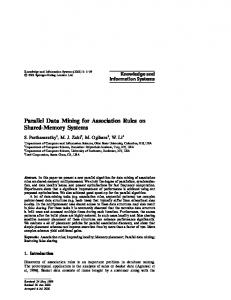
(a) Data Set

(b) Square Wave function

27

(c) Gaussian function

Figure 2.1.1: Examples for influence functions of Denclue. each other, and the density of a data object is the sum of influence functions from all data objects in the data set. By assigning different influence functions, Denclue is a generalization of many partition-based, hierarchical, and density-based clustering methods. Figure 2.1.1 illustrates the effect of different influence functions. Denclue is robust to large amount of noise and works well for high-dimentional data sets. However, it outputs all clusters at the same level. Therefore, it cannot support an exploration of hierarchical cluster structures which exploits users’ domain knowledge.

Subspace Clustering

Clustering in high dimensional space is often problematic as theoretical results [16] questioned the meaning of closest matching in high dimensional spaces. Recent research work [2, 4, 6, 22, 44] has focused on discovering clusters embedded in the subspaces of a high dimensional data set. This problem is known as subspace clustering. Based on the measure


28

of similarity, there are two categories of clustering model.

The first category is pattern-based clustering. A pattern-based cluster[20, 58, 66, 84, 88] consists of a subset of objects O and a subset of attributes A such that O exhibit coherent patterns on A. In pattern-based clustering, the subsets of attributes for various pattern-based clusters can be different. Two pattern-based clusters can share some common objects and attributes, and some objects may not belong to any pattern-based cluster.

Cheng et al. [20] introduced the bicluster concept to model a block, along with a score called the mean-squared residue to measure the coherence of genes and conditions in the block. Given a subset of objects I and a subset of attributes J, the coherence of the submatrix (I, J) is measured by the mean squared residue score. rIJ =

(2.1.2)

1 (ai j − aiJ − aI j + aIJ )2 , ∑ |I||J| i∈I, j∈J

where (2.1.3)

aiJ =

1 |J|

∑ ai j , j∈J

aI j =

1 ai j , |I| ∑ i∈I

and aIJ =

1 ∑ ai j |I||J| i∈I, j∈J

are the average value of row i, the average value of column j, and the average value of the submatrix (I, J), respectively. A submatrix is called a δ-bicluster if H(G0 , S0 ) ≤ δ for some δ > 0. A low mean-squared residue score together with a large variation from the constant suggest a good criterion for identifying a block.

Since the problem of finding a minimum set of biclusters to cover all the elements in a data


29

matrix has been shown to be NP-hard, a greedy method which provides an approximation of the optimal solution and reduces the complexity to polynomial-time has been introduced in [20]. To find a bicluster, the score H is computed for each possible row/column addition/deletion, and the action that decreases H the most is applied. If no action will decrease H or if H ≤ δ, a bicluster is returned. However, this algorithm (the brute-force deletion and addition of rows/columns) requires computational time O((n+m)·mn), where n and m are the number of genes and samples, respectively, and it is time-consuming when dealing with a large gene expression data sets. A more efficient algorithm based on multiple row/column addition/deletion (the biclustering algorithm) with time-complexity O(mn) was also proposed in [20]. After one bi-cluster is identified, the elements in the corresponding sub-matrix are replaced (masked) by random numbers. The bi-clusters are successively extracted from the raw data matrix until a pre-specified number of clusters have been identified. However, the biclustering algorithm also has several drawbacks. First, the algorithm stops when a pre-specified number of clusters have been identified. To cover the majority of elements in the data matrix, the specified number is usually large. However, the biclustering algorithm does not guarantee that the biclusters identified earlier will be of superior quality to those identified later, which adds to the difficulty of the interpretation of the resulting clusters. Second, biclustering “mask” the identified biclusters with random numbers, preventing the identification of overlapping biclusters. δ-Cluster. Yang at al. [88] present a pattern-based clustering method named “δ-clusters”


30

to capture K embedded subspace clusters simultaneously. They use average residue across every entry in the sub-matrix to measure the coherence within a submatrix. A heuristic move-based method called FLOC (FLexible Overlapped Clustering) is applied to search K embedded subspace clusters. FLOC starts with K randomly selected sub-matrices as the subspace clusters, then iteratively tries to add/remove each row/column into/out of the subspace clusters to lower the residue value, until a local minimum residue value is reached. The time complexity of the δ-clusters algorithm is O((n + m) ∗ n ∗ m ∗ k ∗ l), where k is the number of clusters and l is the number of iterations. δ-clusters algorithm also requires the number of the clusters be pre-specified. The advantage of the “δ-clusters” approach is that it is robust to missing values since the residue of a submatrix only computed by existing values. “δ-clusters” can also detect overlapping embedded subspace clusters. In [84], Wang et al. propose the model of δ-pCluster. To constrain the coherence of patterns in a cluster C, δ − pCluster requires the change of differences of any two data objects x, y in C on any two attributes a, b in C should be smaller than a threshold δ. To be formal, let O be a subset of objects in the database (O ⊆ D), and let T be a subset of a subset of attributes (T ⊆ A. Pair (O, T) specifies a submatrix. Given x, y ∈ O, and a, b ∈ T, the pScore of the 2 × 2 matrix is defined as  (2.1.4)

 dxa pScore(  dya

 dxb  ) = |(dxa − dxb ) − (dya − dyb )|  dyb

Pair (O, T) forms a δ− pCluster if for any 2×2 submatrix X in (O, T), we have pScore(X) ≤


31

δ for some δ > 0. In a recent study [66], Pei et al. develop MaPle, an efficient algorithm to mine the complete set of non-redundant pattern-based clusters.

OP-Cluster. In [58], Liu et al. present the model of OP-Cluster. Under this model, the coherence within a cluster is constrained by the relative order of the attribute values of the objects within the cluster. To be specific, an object O shows the “UP” pattern on a permutation A0 = {ai1 , . . . , ain } of attributes A = {a1 , . . . , an } if the attribute values hdi1 , . . . , din i of O on A0 is in a “non-decreasing” order. Let O be a subset of objects in the database (O ⊆ D), and let T be a subset of a subset of attributes (T ⊆ A. Pair (O, T) forms a Order Preserving Cluster (OP-Cluster) if there exists a permutation of attributes in T, on which every object in O shows the “UP” pattern. In practice, the requirement of “non-decreasing order” is often relaxed by a group function. In [58], an efficient algorithm, OPC-Tree, is proposed to find the OP-Clusters. Both MaPle and OPC-Tree guarantee to find the complete set of the pattern-based clusters in the data set.

The second category is distance-based clustering. In this category, one of the well known subspace clustering algorithms is CLIQUE [6]. CLIQUE is a density and grid based clustering method. The PROCLUS [4] and the ORCLUS [2] algorithms find projected clusters based on representative cluster centers in a set of cluster dimensions. Another interesting approach, Fascicles [44], finds subsets of data that share similar values in a subset of dimensions.


2.2

32

Cluster Validation

Different clustering algorithms, or even a single clustering algorithm using different parameters, generally result in different sets of clusters. Therefore, it is important to compare various clustering results and select the one that best fits the “true” data distribution. Cluster validation is the process of assessing the quality and reliability of the cluster sets derived from various clustering processes.

A lot of approaches [21, 59, 60, 61] have been proposed for evaluating the results of a clustering algorithm. Various methods have been designed to assess the quality and reliability of clustering results. Each clustering algorithm has its advantages and disadvantages. For a data set with clusters of various size, density, or shape, different clustering algorithms are best suited to detecting clusters of different types in the data set. No single approach combines the advantages of these various clustering algorithms while avoiding their disadvantages.

Generally, cluster validity has three aspects. First, the quality of clusters can be measured in terms of homogeneity and separation on the basis of the definition of a cluster: objects within one cluster are similar to each other, while objects in different clusters are dissimilar with each other. The second aspect relies on a given “ground truth” of the clusters. The “ground truth” could come from domain knowledge, such as known function families of


33

genes, or from other sources such as the clinical diagnosis of normal or cancerous tissues. Cluster validation is based on the agreement between clustering results and the “ground truth”. The third aspect of cluster validity focuses on the reliability of the clusters, or the likelihood that the cluster structure is not formed by chance. In this section, we will discuss these three aspects of cluster validation.

There are various definitions for the homogeneity of clusters which measures the similarity of data objects in cluster C. For example, H1 (C) =

∑Oi ,O j ∈C,Oi 6=O j Similarity(Oi ,O j ) . ||C||·(||C||−1)

This definition represents the homogeneity of cluster C by the average pairwise object similarity within C. An alternate definition evaluates the homogeneity with respect to the “centroid” of the cluster C, i.e., H2 (C) =

1 ¯ ||C|| ∑Oi ∈C Similarity(Oi , O),

where O¯ is

the “centroid” of C. Other definitions, such as the representation of cluster homogeneity via maximum or minimum pairwise or centroid-based similarity within C can also be useful and perform well under certain conditions. Cluster separation is analogously defined from various perspectives to measure the dissimilarity between two clusters C1 , C2 . For example, S1 (C1 ,C2 ) =

∑Oi ∈C1 ,O j ∈C2 Similarity(Oi ,O j ) ||C1 ||·||C2 ||

and S2 (C1 ,C2 ) = Similarity(O¯ 1 , O¯ 2 ).

Since these definitions of homogeneity and separation are based on the similarity between objects, the quality of C increases with higher homogeneity values within C and lower separation values between C and other clusters. Once we have defined the homogeneity of a cluster and the separation between a pair of clusters, for a given clustering result C= {C1 ,C2 , . . . ,CK }, we can define the homogeneity and the separation of


34

C. For example, Sharan et al. [75] used definitions of Have = Save =

1 (||Ci || · ||C j ||)S2 (Ci ,C j ) ∑Ci 6=C j ||Ci ||·||C j || ∑Ci 6=C j

1 N

∑Ci ∈C ||Ci || · H2 (Ci ) and

to measure the average homogeneity

and separation for the set of clustering results C.

If the “ground truth” of the cluster structure of the data set is available, we can test the performance of a clustering process by comparing the clustering results with the “ground truth”. Given the clustering results C = {C1 , ...,C p }, we can construct a n ∗ n binary matrix C, where n is the number of data objects, Ci j = 1 if Oi and O j belong to the same cluster, and Ci j = 0 otherwise. Similarly, we can build the binary matrix P for the “ground truth” P = {P1 , ..., Ps }. The agreement between C and P can be disclosed via the following values:

• n11 is the number of object pairs (Oi , O j ), where Ci j = 1 and Pi j = 1; • n10 is the number of object pairs (Oi , O j ), where Ci j = 1 and Pi j = 0; • n01 is the number of object pairs (Oi , O j ), where Ci j = 0 and Pi j = 1; • n00 is the number of object pairs (Oi , O j ), where Ci j = 0 and Pi j = 0.

Some commonly used indices [37] have been defined to measure the degree of similarity between C and P: n11 + n00 , n11 + n10 + n01 + n00

(2.2.1)

Rand index: Rand =

(2.2.2)

Jaccard coefficient: JC =

n11 , n11 + n10 + n01


35 r

(2.2.3)

Minkowski measure: Minkowski =

n10 + n01 . n11 + n01

The Rand index and the Jaccard coefficient measure the extent of agreement between C and P, while Minkowski measure illustrates the proportion of disagreements to the total number of object pairs (Oi , O j ), where Oi , O j belong to the same set in P. It should be noted that the Jaccard coefficient and the Minkowski measure do not (directly) involve the term n00 . These two indices may be more effective in gene-based clustering because a majority of pairs of objects tend to be in separate clusters and the term n00 would dominate the other three terms in both good and bad solutions. Other methods are also available to measure the correlation between the clustering results and the “ground truth” [37]. Again, the optimal index selection is application-dependent.

2.3

Outlier Detection

Outlier detection is concerned with discovering the exceptional behaviors of certain objects. It is an important branch in the field of data mining with numerous applications, including credit card fraud detection, discovery of criminal activities, discovery of computer intrusion, and etc. In some sense it is at least as significant as cluster detection.


36

There are numerous studies on outlier detection. D. Yu etc. [91] proposed an outlier detection approach termed FindOut as a by-product of WaveCluster [76] which removes the clusters from the original data and thus identifies the outliers by applying signal-processing techniques. E. M. Knorr etc. [54] detected a distance-based outlier which is a data point with a certain percentage of the objects in the data set having a distance of more than dmin away from it. S. Ramaswamy etc. [68] further extended it based on the distance of a data point from its kth nearest neighbor and identified the top n points with largest kth nearest neighbor distances as outliers. M. M. Breunig etc. [19] introduced the concept of local outlier and defined local outlier factor (LOF) of a data point as a degree of how isolated the data point is with respect to the surrounding neighborhood. Aggarwal etc. [5] considered the problem of outlier detection in subspace to overcome dimensionality curse.

2.4

Indexing Multi-Dimensional Data

Recently large volumes of data with high dimensionality are being generated in many fields. Many approaches have been proposed to index high-dimensional data sets for efficient querying. Although most of them can efficiently support nearest neighbor search for low dimensional data sets, they degrade rapidly when dimensionality goes higher. Also the dynamic insertion of new data can cause original structures no longer handle the data sets efficiently since it may greatly increase the amount of data accessed for a query.


37

Among those approaches, the ClusterTree [92] is the first work towards building efficient index structure from clustering for high-dimensional data sets. The ClusterTree approach builds an index structure on the cluster structures to facilitate efficient queries.

Existing multidimensional tree-like indexing approaches can be further classified into two categories: space partitioning and data partitioning.

A data partitioning approach partitions a data set and builds a hierarchy consisting of bounding regions. The bounding regions at higher levels contain the lower regions and the bounding regions at the bottom level contain the actual data points. Popularly used index structures include R-Tree, R∗ -tree, SS-Tree, SS+ -Tree and SR-Tree. An R-tree [36] is a height-balanced tree with index records in its nodes. There are two kinds of nodes: internal and leaf nodes. All the nodes have minimum bounding rectangles (MBR) as page region. R-tree is used to store rectangular regions of an image or a map. R-trees are very useful in storing very large amounts of data on disk. One disadvantage of R-trees is that the bounding boxes (rectangles) associated with different nodes may overlap. The R∗ -tree [11] is an R-tree variant which incorporates a combined optimization of area, margin and overlap of each enclosing rectangle in the tree nodes. It reduces the overlapping between the MBRs of neighboring nodes, reduces the volume of the MBRs and improves the storage utilization.


38

In contrast to the R-Tree, SS-Tree [1] uses hyper-spheres as region units. Each hypersphere is represented by a centroid point, and a radius large enough to contain all of the underlying data points. Queries on the SS-Tree are very efficient because it only needs to calculate similarity between a region and the query point. The SS+ -Tree [56] is a variant of the SS-Tree with a modified splitting heuristic to optimize the bounding shape for each node.

SR-Tree [51] is an index structure which combines the bounding spheres and rectangles for the shapes of node regions to reduce the blank area. The region for a node in it is represented by the intersection of a bounding sphere and rectangle so that the overlapping area between two sibling nodes is reduced. It takes the advantages of both rectangles and spheres. However, the storage required for the SR-Tree is larger than the SS-Tree because the nodes in the SR-Tree need to store the bounding rectangles and bounding spheres. Consequently, the SR-Tree requires more CPU time and more disk accesses than the SSTree for insertions.

Space partitioning approaches recursively divide a data space into disjoint subspaces. KD-B Tree and Pyramid-Tree are this type. The K-D-B Tree [69] partitions a d-dimensional data space into disjoint subspaces by (d − 1)-dimensional hyper-planes which are alternately perpendicular to one of the dimension axes. Due to the disjointness among its nodes at the same level, the K-D-B Tree has the advantage that the search path for querying a data


39

point is unique. The Pyramid-Tree [13]’s main idea is to divide the data space first into 2d pyramids, each sharing the center point as its peak (the tip point of a pyramid). Each pyramid is then sliced into slices parallel to the base of the pyramid, and each slice forms a data page. The range query under this index structure can be efficiently processed for both low- and high-dimensional data sets. However, the partitioning of the Pyramid-Tree can not ensure that the data points in one data page are always neighbors.

Among those approaches, the ClusterTree is the first work towards building efficient index structures from clustering for high-dimensional data sets. The ClusterTree has the advantage of supporting efficient data query for high-dimensional data sets. A ClusterTree is a hierarchical representation of the clusters of a data set. It organizes the data based on their cluster information from coarse level to fine, providing an efficient index structure on the data according to clustering. Like many other structures, it has two kinds of nodes: internal and leaf nodes. The internal nodes include pointers to subculsters of this cluster, the bounding sphere for the subclusters and the number of data points in the subclusters. The leaf nodes contain pointers to the data points. For each cluster, the ClusterTree calculates the following parameters: the number of data points, the centroid c, and the volume of the minimum bounding sphere S. The centroid c = hc1 , c2 , · · · , cd i can be calculated by: (2.4.1)

ci =

∑Nj=1 oj i , 1 ≤ i ≤ d, N

where N is the number of the data points in the cluster and oj i is the i-th value of data


40

point oj in the cluster. Thus, each cluster is represented by a hyper-sphere S. So there may be some empty regions which contain no data, and two bounding hyper-spheres of two different clusters may overlap. We can define the density of the cluster as:

(2.4.2)

number o f points in C volume o f S number o f points in C = . d/2 d

Densityc =

2π r dΓ( d2 )

The gamma function Γ(x) is defined as: (2.4.3)

Γ(x) =

Z ∞

t x−1 e−t dt,

0

where Γ(x + 1) = xΓ(x) and Γ(1) = 1. When the density of a cluster falls below a preselected threshold or the number of the data points in the cluster is larger than a pre-selected threshold, the cluster will be decomposed into several smaller clusters (subclusters).

Chapter 3

A Shrinking-Based Clustering Algorithm

Existing data analysis techniques have difficulty in handling multi-dimensional data. Multidimensional data has been a challenge for data analysis because of the inherent sparsity of the points. In this chapter, we first present a novel data preprocessing technique called shrinking which optimizes the inherent characteristic of distribution of data. This data reorganization concept can be applied in many fields such as pattern recognition, data clustering and signal processing. Then, as an important application of the data shrinking preprocessing, we propose a shrinking-based approach for multi-dimensional data analysis which

41

CHAPTER 3. A SHRINKING-BASED CLUSTERING ALGORITHM

42

consists of three steps: data shrinking, cluster detection, and cluster evaluation and selection. The process of data shrinking moves data points along the direction of the density gradient, thus generating condensed, widely-separated clusters. Following data shrinking, clusters are detected by finding the connected components of dense cells (and evaluated by their compactness). The data-shrinking and cluster-detection steps are conducted on a sequence of grids with different cell sizes. The clusters detected at these scales are compared by a cluster-wise evaluation measurement, and the best clusters are selected as the final result. The experimental results show that this approach can effectively and efficiently detect clusters in both low- and high-dimensional spaces.

3.1

Introduction

The generation of multi-dimensional data has proceeded at an explosive rate in many disciplines with the advance of modern technology. Data preprocessing procedures can greatly benefit the utilization and exploration of real data. Clustering is useful for discovering groups and identifying interesting distributions in the underlying data. In this chapter, we first present a data shrinking technique for preprocessing; then, we propose a cluster detection approach by finding the connected components of dense cells and a cluster evaluation approach based on the compactness of clusters.


43

Data preprocessing is commonly used as a preliminary data mining practice. It transforms the data into a format that will be more easily and effectively processed for the purpose of the users.

There are a number of data preprocessing techniques: data cleaning, data integration, data transformation and data reduction. Data cleaning can be applied to remove noise and correct inconsistencies in the data. Data integration merges data from multiple sources into a coherent data store. Data transformation may improve the accuracy and efficiency of mining algorithms involving distance measurements. Data reduction can reduce the data size. These data processing techniques, when applied prior to mining, can substantially improve the overall quality of the patterns mined and/or the time required for the actual mining[47].

Cluster analysis is used to identify homogeneous and well-separated groups of objects in databases. The need to cluster large quantities of multi-dimensional data is widely recognized. It is a classical problem in the database, artificial intelligence, and theoretical literature, and plays an important role in many fields of business and science.

Each of the existing clustering algorithms has both advantages and disadvantages. The most common problem is rapid degeneration of performance with increasing dimensions [42], particularly with approaches originally designed for low-dimensional data.

The

difficulty of high-dimensional clustering is primarily due to the following characteristics of


44

high-dimensional data:

1. High-dimensional data often contain a large amount of noise (outliers). The existence of noise results in clusters which are not well-separated and degrades the effectiveness of the clustering algorithms. 2. Clusters in high-dimensional spaces are commonly of various densities. Grid-based or density-based algorithms therefore have difficulty choosing a proper cell size or neighborhood radius which can find all clusters. 3. Clusters in high-dimensional spaces rarely have well-defined shapes, and some algorithms assume clusters of certain shapes. For example, the algorithms in [64, 93] can efficiently find convex or spherical clusters, but they fail to detect non-spherical clusters because of their specific definition of similarity criteria. 4. The effectiveness of grid-based approaches suffer when data points are clustered around a vertex of the grid and are separated in different cells, as shown in Figure 3.1.1. In the d-dimensional space Rd , there may be 2d points distributed in this manner. The cluster formed by these points will be ignored because each of the cells covering the cluster is sparse.

There are also other algorithms related to data movement[82, 23], however, the existing ones are not suitable for the high dimensional data of large size because based on their


a

b

d

c

45

Figure 3.1.1: Points a, b, c, and d are located near a vertex of the grid and are separated in four neighboring cells. The four neighboring cells contain no other points. definition, the time to run their process is O(n2 ∗ p) where n is the size of the input data and p is the number of iterations in the iterative process. So they are very time-consuming.

A lot of approaches [21, 59, 60, 61] have been proposed for evaluating the results of a clustering algorithm. Each clustering algorithm has its advantages and disadvantages. For a data set with clusters of various size, density, or shape, different clustering algorithms are best suited to detecting clusters of different types in the data set. No single approach combines the advantages of these various clustering algorithms while avoiding their disadvantages.

3.1.1

Proposed approach

In this chapter, we first present a novel data preprocessing technique named shrinking which optimizes the inherent characteristic of distribution of data. For a real data set, the natural data groups (if existing) it contains may be very sparse. In the data preprocessing


46

step, if we could make data points move towards the centroid of the data groups they belong to, the natural sparse data groups will become denser, thus easier to be detected, and noises can be further isolated. Intuitively, a dense area “attracts” objects in sparse areas surrounding it, and becomes denser. Here we assume a data point is attracted to neighboring data points, and it moves towards the way the attraction is the strongest. In other words, the direction it is attracted to is determined by the distribution of its neighboring data points. Our data shrinking preprocessing computes a simulated movement of each data point in a data set that reflects its “attraction” to neighboring data points. We can also refer to the concept of infiltration mechanism[85] in which materials such as water move from denser areas to sparser ones whereas in our case, the data point will move to a denser area nearby. When computing the attraction on a data point, those points far away from this data point can be ignored due to the little effect they impose on it. This data reorganization concept can be applied in many fields such as pattern recognition, data clustering and signal processing to facilitate a large amount of data analysis categories.

Then, as an important application of the data shrinking preprocessing, we propose a shrinkingbased approach for multi-dimensional data analysis to address the inadequacies of current clustering algorithms in handling multi-dimensional data. This clustering method is combined with a cluster-wise evaluation measurement to select the best clusters detected at different scales.


47

The proposed algorithm consists of three steps which are data shrinking, cluster detection, and cluster evaluation and selection. In the data-shrinking step, data points move along the direction of the density gradient, leading to clusters which are condensed and widely-separated. Following data shrinking, clusters are detected by finding the connected components of dense cells. The data-shrinking and cluster-detection steps are grid-based. Instead of choosing a grid with a fixed cell size, we use a sequence of grids of different cell sizes. Our technique also includes a method to avoid the problem caused by points clustered near a vertex of a grid and separated in different cells, as shown in Figure 3.1.1. For each cell size, the processes of data shrinking and cluster detection are performed on two interleaved grids. Then, in the cluster evaluation and selection step, we evaluate clusters detected at different scales via a cluster-wise evaluation measurement and select the best clusters as the final result.

Although the idea of moving data points according to the density gradient has been around quite some time [48], this chapter distinguishes mainly in the following two aspects:

• A grid-based shrinking and evaluation approach is proposed. Instead of choosing a grid with a fixed cell size, we use a sequence of increasing grid sizes to catch the cluster structures of the input data in different scales. At each scale, two grids are used, the second one is shifted diagonally from the first one.


48

• We integrate a compactness-based cluster evaluation into the framework. The compactnessbased evaluation computes both inter-cluster and intra-cluster distances (which model the inter-cluster and intra-cluster relationships, respectively) and evaluate a cluster’s compactness with the ratio of the second distance to the first one.

The remainder of this paper is organized as follows. Section 3.2 introduces methods for the selection of multiscale grids for use in data shrinking and cluster detection. Section 3.3 discusses the data-shrinking process. In Section 3.4, a simple grid-based cluster detection method is presented. In Section 3.5, we discuss our definition of compactness as pertains to evaluating and selecting clusters. Section 5.4 presents experimental results, and concluding remarks are offered in Section 7.1.

3.2

Choosing Grid Scales for the Shrinking-based Clustering Approach

To demonstrate the advantages of the data shrinking preprocessing, we applied it to the multi-dimensional clustering problem which plays an important role in many fields of business and science. We propose a grid-based approach to data shrinking and cluster detection.


49

Choosing grids: Grid-based clustering methods depend heavily on the proper selection of grid-cell size. Without prior knowledge of the structure of an input data set, proper grid-cell size selection is problematical. We propose a multiscale gridding technique to address this problem. Instead of choosing a grid with a fixed cell size, we use a sequence of grids of different cell sizes. Data shrinking and cluster detection are conducted on these grids, the detected clusters are compared, and those clusters with the best quality are selected as the final result.

Throughout this paper, we assume that the input data set X is X = {~X1 , ~X2 , ..., ~Xn }, which is normalized to be within the hypercube [0, 1)d ⊂ Rd .

We apply a simple histogram-based approach to get reasonable grid scales for the datashrinking process. We scan the input d-dimensional data set X once and get the set of histograms, one for each dimension: H = {h1 , h2 , ..., hd }.

Each bin of a histogram denotes the number of data points in a certain segment on this histogram. We set up a number β as a quantity threshold. It is used in the following algorithm to help


50

generate density spans. Here we first give the definition of density span which will help understand the algorithm:

Definition 1: A density span is a combination of consecutive bins’ segments on a certain dimension in which the amount of data points exceeds β. A size of a density span is the sum of the sizes of the bins it includes.

For each histogram hi , i=1,...,d, we sort its bins based on the number of data points they contain in descending order. Then we start from the first bin of the ordered bin set and merge it with its neighboring bins until the total amount of data points in these bins exceeds β. At each step, we check the number of points in the bin on the left side and the one on the right side of the currently span, and choose the bin with more points in it to merge with. Thus a density span is generated as the combination of the segments of these bins. If a current span has less than β data points, but its left and right neighbors have both been assigned to a precious span already, we stop the operation on the current span and call it as an incomplete span which will not be considered in the following procedure of generating multiple grid scales. The operation is continued until all the non-empty bins of this histogram is in some density spans or some incomplete spans. Each histogram has a set of density spans.

Figure 3.2.1 shows an example of this density span generation operation. Here we just demonstrate two density spans on this histogram. Bin 21 is the one with largest amount of


51

Figure 3.2.1: An example of density span acquirement data points. We start from Bin 21, check its neighboring bins 20 and 22, and choose bin 20 to merge with because it has more points than bin 22. Next we check the neighboring bins of the combination of the segments of bin 20 and 21, which are bin 19 and bin 22, and choose bin 19 because it has more points than bin 22. In this way the neighboring bins are merged until the amount of data points included exceeds β. Thus density span 1 is generated. Bin 7 has the second largest amount of data points. Density span 2 is generated starting from bin 7, first including bin 8, then including bin 6, 9, 10 and 5, step by step until the amount of data points included exceeds β.

After the density span generation operation mentioned above, we have a set T of density spans with different sizes. We cluster the density spans by their sizes. We do the procedure


52

as follows. First we sort the sizes by ascending order. Then starting from the smallest size so , we include the current size into cluster T1 until we come across a size s0 such that s0 − so > so ∗ 5%. Then we start from s0 and do the same procedure to get cluster T2 , and so on. For each cluster Ti , we denote the number of sizes in it as Ni , and denote the average value of the sizes in it as Si . we sort Si based on Ni by descending order and choose first Ks ones as the multiple scales for the following data shrinking and cluster detection procedures. In other words, those sizes of density spans which appear often are chosen. Algorithm 1 describes the procedure of the density span generation on a certain dimension. The value β depends on the size of the input data set X. Normally it can be set as a certain percentage of the number of data points in X. There is a balance in choosing a value for Ks : a smaller Ks can increase the precision of cluster detection, while a larger Ks can save time. The time complexity for this method is determined by the dimensionality d of X and the amount of bins Bn in each histogram. The time required to perform Algorithm 1 is O(Bn log Bn ).


53

Algorithm 1 (Density span generation) Input: histogram hi Output: Density span set of hi 1) Sort the bins of hi in the descending order; 2) Beginning from the first bin of the ordered bin set, merge it with its neighbors until the total amount of data points included exceeds β; 3) Repeat step 2 until all non-empty bins are included in some density spans or some incomplete spans; 4) Output the density span set.

The multiscale gridding scheme proposed above not only facilitates the determination of a proper cell size but also offers advantages for handling data sets with clusters of various densities. For example, the data set in Figure 3.2.2 has three clusters. The two clusters on the left have higher densities than the cluster on the right. The grid with a smaller cell size (shown in solid lines) can distinguish the left two clusters but fails to detect the right cluster, while the converse is true for the grid with a larger cell size (shown in dashed lines). For data sets of this kind, a multiscale gridding method is needed to distinguish all clusters.


54

Figure 3.2.2: A data set with three clusters

3.3

Data Shrinking

We start with the first step of the proposed method: data shrinking. In this step, each data point moves along the direction of the density gradient and the data set shrinks toward the inside of the clusters. Points are “attracted” by their neighbors and move to create denser clusters. This process is repeated until the data are stabilized or the number of iterations exceeds a threshold.

The neighboring relationship of the points in the data set is grid-based. The space is first subdivided into grid cells. Points in sparse cells are considered to be noise or outliers and will be ignored in the data-shrinking process. Assume a dense cell C with neighboring cells surrounding C. Data shrinking proceeds iteratively; in each iteration, points in the dense cells move toward the data centroid of the neighboring cells. The iterations terminate if


55

the average movement of all points is less than a threshold or if the number of iterations exceeds a threshold.

The major motivation for ignoring sparse cells is computation time. If the grid cells are small, the number of non-empty cells can be O(n), where n is the number of data points. The computation of data movement for all non-empty cells takes a length of time quadratic to the number of non-empty cells, which is O(n2 ). By ignoring sparse cells in the data movement, dramatic time savings can be realized.

3.3.1

Space subdivision

Given the side length

1 κ

of grid cells, the hypercube [0, 1)d is subdivided into κd cells:

i1 i1 + 1 i2 i2 + 1 id id + 1 {C(i1 , i2 , ..., id ) = [ , )×[ , ) × ... × [ , )|i1 , i2 , ..., id ∈ {0, 1, ..., κ − 1}}. κ κ κ κ κ κ

Each cell C(i1 , i2 , ..., id ) has a unique ID: (i1 , i2 , ..., id ). Two distinct cells C(i1 , i2 , ..., id ) and C( j1 , j2 , ..., jd ) are neighboring cells if |ik − jk | ≤ 1 for all k = 1, 2, ..., or d. The neighboring cells of a cell C are also called the surrounding cells of C. This arrangement is shown in Figure 3.3.1. For each data point ~Xi , the cell containing the point can be easily found; this cell is denoted


56

C

Figure 3.3.1: Surrounding cells (in gray) of the cell C (in black) as Cell(~Xi ). We then sort the data points into their cells to find all nonempty cells and the points contained by each. For each nonempty cell, we compute its density, defined as a fraction of the number of points in the cell over the volume of the cell. A cell is called a sparse/dense cell if its density is less/not less than a density threshold Tdn1 . The selection of the density threshold Tdn1 will be discussed in Subsection 4.2.3, below. Points in sparse cells are considered to be noise or outliers and will be ignored in the data-shrinking process. We then denote the set of dense cells as (3.3.1)

DenseCellSet = {C1 ,C2 , ...,Cm }.

For each dense cell C, the centroid of its points is computed: Σkj=1~Xi j (3.3.2) DataCentroid(C) = , k where {~Xi j }kj=1 is the set of points in the cell. It is called the data centroid of the cell C. Each dense cell contains its own points and data centroid. The computational process involved in finding the dense cells, their points, and their centroids takes time O(n log n). The space occupied by the dense cells is O(n).


57

In high-dimensional spaces, ignoring the sparse cells can be problematical. Figure 3.3.2(a) illustrates four points in a two-dimensional grid. The four points are clustered near a vertex of the grid and are separated in four neighboring cells. In the d-dimensional Euclidean space Rd , there may be 2d points distributed in a similar manner. These points should have an influence on the data-shrinking process but will be ignored because they are separated in different cells. To address this issue, we choose two interleaved grids for a given cell size. An example of such interleaved grids is given in Figure 3.3.2(a) and (b).

a

b

d

c

(a)

(b)

(c)

Figure 3.3.2: (a) Points a, b, c, and d are located near a vertex of the grid and are separated in four neighboring cells; (b) another grid with the same cell size; (c) the two grids (shown respectively by solid and dashed lines) in the same plane.

The idea of using several shifted grids to improve the histograms accuracy was first published in 1985 by D.W. Scott [26]. When handling data of large size, effectiveness and efficiency are always the two main goals we need to achieve and balance. Regarding the shifted grids, 2d shifted grids are needed to ensure that we get a dense cell for each clustered point set. However, that’s practically infeasible.

We choose two grids at each scale with the second one shifted diagonally from the first one because it will improve the efficiency of our algorithm. Also the diagonally shifted


58

grid best complements the original one (as compared with each individual other), though the complement is not complete. Realizing the problem of the incompleteness, we used a sequence of grid sizes.

In [65] a random selection of shifts has been used. However, to balance the effectiveness and efficiency, this approach has to make a decision on how many shifts will be used. Our approach attempts to handle this problem by changing grid sizes, which has two advantages: (1) It can also be used for catching the cluster structures in different scales. (2) When choosing a sequence of grid sizes, we used the approach of density span generation (Algorithm 1). As a comparison, the random-selection-of-shift approach has to choose among 2d possible shifts to find the properly shifted grids.

3.3.2

Data movement in a single iteration

Data movement is an iterative process intended to move data gradually toward a goal of increased cluster density. This data-movement process is conducted alternately on two interleaved grids in alternating iterations.

In each iteration, points are “attracted” by their neighbors and move toward the inside of the clusters. Each point in a cell C has neighboring points in C or in the cells surrounding C. The movement of a point can be intuitively understood as analogous to the attraction of


59

a mass point by its neighbors. Thus, the point moves toward the centroid of its neighbors. However, data movement thus defined can cause an evenly-distributed data set to be condensed in a piece-wise manner. For example, for each point in Figure 3.3.3(a), the centroid of its neighbors is in the center of a grid cell, causing all points to be attracted to the centers of the grid cells. After the data-movement procedure, the data set in Figure 3.3.3(a) becomes the isolated points shown in Figure 3.3.3(b).

(a)

(b)

Figure 3.3.3: A part of a data set (a) before movement and (b) after movement. The arrows in (a) indicate the direction of motion of the points. The grid cells are shown in dashed lines.

Our solution to the above problem is to treat the points in each cell as a rigid body which is pulled as a unit toward the data centroid of those surrounding cells which have more points. Therefore, all points in a single cell participate in the same movement. This approach not only solves the problem of piece-wise condensing but also saves time.

Formally, suppose the data set at the beginning of ith iteration becomes {~X1i , ~X2i , ..., ~Xni },


60

and the set of dense cells is (3.3.3)

DenseCellSet i = {C1i ,C2i , ...,Cmi }.

Respectively, we assume that the dense cells have n1 , n2 , ..., nm , points and their data centroids are (3.3.4)

~Φ1 , ~Φ2 , ..., ~Φm .

For a dense cell Cij , we suppose that its surrounding dense cells are Cijk , for k = 1, 2, ..., w. Then the data centroid of these surrounding cells is (3.3.5)

~ Σw k=1 n jk × Φ jk , w Σk=1 n jk

which is denoted as ~Φsj . The movement for cell Cij in the ith iteration is

(3.3.6)

   ~Φs − ~Φ j i f k ~Φs − ~Φ j k≥ Tmv × 1   j j κ    Movement(Cij ) = and Σw k=1 n jk > n j ;       0 otherwise,

where k ~Φsj − ~Φ j k is the distance between the two centroids ~Φsj and ~Φ j , Tmv is a threshold to ensure that the movement is not too small, and

1 κ

is the side length of grid cells, as

discussed in the last subsection of this section. Tmv is usually a number between 0.5 and 0.5 ×

√

d. Formula 3.3.6 states that, if the distance between ~Φsj and ~Φ j is not too small

and the surrounding cells have more points, then cell Cij will be translated such that its


61

data centroid is moved to the data centroid of the surrounding dense cells; otherwise, cell Cij remains static. The movement for each cell indicates the approximate direction of the density gradient around the cell. After movement, a data point ~X in cell Cij is moved to ~X + ~Φsj − ~Φ j . To compute the movement for a dense cell Cij , we browse the set of dense cells to find its surrounding cells and then calculate the movement. The computation takes O(m) time. It then takes O(n j ) time to update the points in the cell. Therefore in the ith iteration, the time used to move all points is O(m2 + n). Thus, the time required for the ith iteration is O(m2 + n log n), where O(n log n) time is used for the subdivision of space.

3.3.3

Termination of shrinking

Ideally, for a data set covering a manifold with a boundary, the shrinking process pushes the boundary points inward until the manifold is reduced to its skeleton. If the skeleton is also a manifold with a boundary, it is skeletonized again. This process is repeated until a manifold with no boundary is produced, as shown in Figure 3.3.4. However, most data sets from real-world applications do not have well-defined shapes in high-dimensional spaces. The data sets resulting from the shrinking process may also not have well-defined shapes. In general, the shrinking process produces individual clusters which are condensed and therefore widely separated, facilitating cluster detection.


62

Figure 3.3.4: Repeated skeletonization. The average movement of all points in each iteration is checked to determine the stability of the data set. Suppose that in the ith iteration, the movements for the n points are~v1 ,~v2 , ...,~vn , respectively. Then the average movement is

Σnj=1 k~v j k . n

If the average movements for two

consecutive iterations are both less than Tamv , where Tamv is a threshold, then the data set is considered stabilized and the shrinking process is terminated.

Due to the complicated high-dimensional structures in most real data, it would be a very challenging problem, if solvable, to give a theoretical analysis of the number of iterations needed for the real data to get stabilized. To control the total computation time, we set a upper bound, Tit , for the number of iterations. If the number of iterations exceeds Tit before the data is stabilized, then the shrinking process is also terminated.

3.3.4

Time and space analysis

Throughout the shrinking process, we need to keep track of the locations of all points, which collectively occupy O(n) space. Data points are assigned to grid cells. Each dense grid cell serves as a container for its points, together with their centroid and movement. The data structure represented by the dense cells occupies O(n) space; therefore, the total


63

space needed is O(n). The time required for each iteration is O(m2 + n log n), where m is the number of dense cells. Since the maximum number of iterations is Tit , the total running time is O(Tit (M 2 + n log n)), where M is the maximum number of dense cells in all iterations.

The value M, representing the maximum number of dense cells, has a significant impact on running time. M can be controlled through the selection of a density threshold Tdn1 . The number of data points in a dense cell must be no less than the product of Tdn1 and the volume of the cell, or Tdn1 × ( κ1 )d . Thus the number of dense cells must not exceed ˜ we can choose a value Tdn1 such that a desired value M,

n Tdn1 ×( κ1 )d

n . Tdn1 ×( κ1 )d

Given

˜ thus ensuring that ≤ M,

˜ However, if the densities of most cells happen the number of dense cells will not exceed M. to fall below a threshold Tdn1 chosen via this method, the data-shrinking process will be unproductive. Alternatively all non-empty cells can be sorted by the number of data points they contain. The density threshold Tdn1 is then chosen so that the first M˜ cells are dense cells. Cases may occur where, for a given grid-cell side length κ1 , most non-empty cells will be very sparse, containing only one or two points each. In such instances, the side length 1 κ

is too small and a larger-scale grid should be used. This is due to the fatal weakness of

grid-based approach for high-dimensional data analysis. As we discussed previously in this section, unless 2d shifted grids are used, it is not guaranteed to have a dense cell for each clustered point set, which makes such a case possible: while the input data set has clusters, it appears sparsely in all cells of the chosen grids. A possible solution to this problem is to


64

combine the grid-based approach with a nearest-neighbor search and use the result from a nearest-neighbor search to choose proper grids. Due to the limited pages of this paper, we cannot investigate this in more details.

3.4

Cluster detection

The second step of our method is cluster detection. Since the data-shrinking process generates individual clusters which are condensed and widely separated, it can be used as a preprocessing with any cluster-detection algorithm. In this paper, we use a simple gridbased cluster-detection method to test the data-shrinking process. For a given cell-side length κ1 , after the data-shrinking process is performed on the input data set, we find the dense cells. Neighboring dense cells are connected and a neighborhood graph of the dense cells is constructed. Each connected component of the neighborhood graph is a cluster.

The cluster-detection method is conducted on two interleaved grids. This avoids the problem caused by points clustered near a vertex of a grid and separated in different cells, as discussed in Subsection 3.3.1. Let Tdn2 be a density threshold. A cell in either of the two interleaved grids is called a dense cell if its density is no less than Tdn2 . Let DC1 and DC2 be the dense cell sets of the two interleaved grids, respectively. Two cells


65

T

C1 ∈ DC1 and C2 ∈ DC2 are called neighbors if C1 C2 6= Ø. The neighborhood graph of dense cells, G, is a pair G =< DC1 DC1

S

S

DC2 , E >, where E is the set of neighboring pairs in

DC2 . The edge set E can be represented by a matrix. Let |DC1 | = m1 , |DC2 | = m2 ,

and DC1

S

m1 +m2 DC2 = {Ci }i=1 . Then E = (Ei j )(m1 +m2 )×(m1 +m2 ) , where

(3.4.1)

Ei j =

    1 if Ci and C j are neighbors;    0 otherwise.

We then run a breadth-first search algorithm (see pages 469-472 in [24]) to find the components of graph G.

The time and space required for the breadth-first search algorithm are both O(|DC1

S

DC2 |+

|E|). To construct graph G, the time and space needed are O((m1 + m2 )2 ). The total time and space required for the cluster-detection algorithm are therefore O((m1 + m2 )2 ). Since the data-shrinking process is performed first, the number of dense cells, defined as m1 + m2 , is greatly reduced, which makes our cluster-detection algorithm particularly useful for real data sets of large size.


3.5

66

Cluster evaluation and selection

After the cluster detection step, we evaluate the clustering results. There are several ways to define what is a good clustering ([53] .etc). Most conventional clustering validity measurements [21, 59, 60, 61] evaluate clustering algorithms by measuring the overall quality of the clusters. However, each clustering algorithm has its advantages and disadvantages. For a data set with clusters of various sizes, densities, or shapes, different clustering algorithms are best suited to detecting the clusters of different types in the data set. No single approach combines the advantages of the various clustering algorithms while avoiding their disadvantages. In this section, we introduce a cluster-wise measurement which provides an evaluation method for individual clusters.

A cluster in a data set is a subset in which the included points have a closer relationship to each other than to points outside the cluster. In the literature [21, 59], the intra-cluster relationship is measured by compactness and the inter-cluster relationship is measured by separation. Compactness is a relative term; an object is compact in comparison to a looser surrounding environment. We use the term compactness to measure the quality of a cluster on the basis of intra-cluster and inter-cluster relationships. This definition of compactness is used to evaluate clusters detected at different scales and to then select the best clusters as the final result.


3.5.1

67

Compactness graphing

We first define compactness in a weighted graph. Then we give an algorithm to compute compact subsets and prove that the compactness defined in a graph is equivalent to that defined in its minimal spanning tree. Thus the problem of finding compact subsets (i.e. clusters) in a graph is reduced to compute its minimal spanning tree. Let G =< V, E > be a fixed graph, where V is the vertex set and E is the edge set. Let w : E → R+ be a weight function on the edge set. We use the terms internal connecting distance (ICD) and external connecting distance (ECD) to measure the closeness of the internal and external relationships, respectively. Compactness is then defined as the ratio of the external connecting distance over the internal connecting distance.

Definition 2: For any graph G =< V, E > with positive weight function w, and any connected1 subset T ⊆ V , let L = {w(p, q) | (p, q) ∈ E, p ∈ T, q 6∈ T }. We define the external connecting distance of T with respect to G as: ECD(T ; G, w) = min L. If L is empty, then define ECD(T ; G, w) to be infinite.

In the above definition, ”min L” denotes the minimum number in set L.

Definition 3: For any graph G =< V, E > with positive weight function w, and any connected subset T ⊆ V , let L = {l ∈ R+ |X}. where X = hT, {(p, q) ∈ E|p ∈ T, q ∈ T, w(p, q) ≤ 1T

is connected means subgraph < T, {(p, q) ∈ E|p, q ∈ T } > is connected.


68

l}i) is a connected subgraph o f G. We define the internal connecting distance of T with respect to G as: ICD(T ; G, w) = inf L.

In the above definition, ”inf L” denotes greatest lower bound of set L.

ECD(T ; G, w) gives the length of a shortest edge connecting T and V − T . ICD(T ; G, w) gives the shortest length to “maintain” T connected. It is easy to see that ECD(T ; G, w) is infinite iff T is a connected component of G, and for any connected subset T , ICD(T ; G, w) is finite, and there is a connected subgraph < T, H > such that all edges in H have weights no more than ICD(T ; G, w).

Definition 4: For any graph G =< V, E > with positive weight function w, and any connected subset T ⊆ V , we define T’s compactness as Compactness(T ; G, w) =

ECD(T ;G,w) ICD(T ;G,w) .

T is compact (or T is a cluster) if its compactness is greater than 1, i.e., ECD(T ; G, w) > ICD(T ; G, w). We denote the set of all clusters in G as ClusterSet(G,w).

Algorithm 2 is an algorithm to calculate all clusters in a weighted graph. This algorithm works similarly to connected-component-finding algorithms. In the beginning, each vertex is a component. Then starting from the shortest edge, we merge these components with edges in the order of weight-ascending. Each edge connecting two components will merge the two components into one. In the merging process, output the components with compactness greater than one.


69

We have following theorem to guarantee that the above algorithm is correct.

Theorem 1: For any graph G =< V, E > with positive weight function w, let C be the output of ClusterFinding(G, w). Then we have: C = ClusterSet(G, w).

Proof: First we prove C ⊆ ClusterSet(G, w), i.e., for any P ∈ C, P ∈ ClusterSet(G, w).

If P appears in the final D, i.e., P is added to C by the operation of line 14, then P is a connected component of G, thus it is a cluster, i.e., P ∈ ClusterSet(G, w). From now on, suppose P ∈ C doesn’t appear in the final D. Then P is added to C by the operation of line 8 or 9. It is obvious that for such P, ecl(P) < ∞, icl(P) < ∞. To prove P ∈ ClusterSet(G, w), it suffices to prove ecl(P) = ECD(P; G, w) and icl(P) = ICD(P; G, w).

To prove ecl(P) ≥ ECD(P; G, w), by the algorithm, there is some (p, q) ∈ E such that p ∈ P ∈ D, q ∈ Q ∈ D, P 6= Q, and w(p, q) = ecl(P). It is obvious that at all time, D is a subdivision of V . So q 6∈ P. By the definition of ECD, we have ecl(P) ≥ ECD(P; G, w).

Here we do not present the proof of ecl(P) = ECD(P; G, w), icl(P) = ICD(P; G, w), and


70

we omit the proof of ClusterSet(G, w) ⊆ C.

2

Algorithm 2 (ClusterFinding(G,w)) Input: G =< V, E >, w : V → R+ Output: C, the set of all clusters in G 1) Let D = {{p}|p ∈ V }; 2) Let ecl : D −→ R+ be a function; 3) Let icl : D −→ R+ be a function; 4) Sort E by the weights of all edges in ascending order; 5) For each edge (p,q) ∈ E, if p ∈ P ∈ D, q ∈ Q ∈ D and P 6= Q, 6)

let ecl(P) = ecl(Q) = w(p, q);

7)

if ecl(P) > icl(P), add P to C;

8)

if ecl(Q) > icl(Q), add Q to C;

9)

remove P, Q from D; Add P Q to D;

10)

S

S

let icl(P Q) = w(p, q);

11)For each X ∈ D, 12)

let ecl(X) = ∞;

13)

add X to C; //Connected components are trivial clusters

14) Output C;

Corollary 1: For any graph G =< V, E > with positive weight function w, and any P ∈


71

ClusterSet(G, w), we have ECD(P; G, w) = ecl(P) and ICD(P; G, w) = icl(P), where ecl, icl are functions defined in Algorithm 2.

If we compare Algorithm 2 and Kruskal’s algorithm for computing minimal spanning tree (See page 505 of [24]), we can find that for each edge e = (p, q) ∈ E, if it is not in the minimal spanning tree given by Kruskal’s algorithm (i.e., when (p, q) is processed, p, q are in the same component in D) , then e has no effect to the output of Algorithm 2. Then we get following corollary.

Corollary 2: For any graph G =< V, E > with positive weight function w, let SG =< V, SE > be a minimal spanning tree of G, and sw = w|SE : SE → R+ . Then we have (1) ClusterSet(G, w) = ClusterSet(SG, sw); and (2) ∀P ∈ ClusterSet(G, w),Compactness(P; G, w) = Compactness(P; SG, sw). For any finite point set V in Euclidean space Rn , a minimal spanning tree of its complete graph is always a subgraph of its Delaunay graph. So we have following result. Corollary 3: For any finite point set V in Euclidean space Rn , let G = (V, E) be its complete graph, and DG = (V, DE) be its Delaunay neighborhood graph. For any p, q ∈ Rn , let dE (p, q) be the Euclidean distance between p, q. Then we have (1) ClusterSet(G, dE ) = ClusterSet(DG, dE ); and (2) ∀P ∈ ClusterSet(G, dE ),Compactness(P; G, dE ) = Compactness(P; DG, dE ).


72

From Algorithm 2, we can easily see that any two clusters don’t intersect if one doesn’t include the other.

Corollary 4: For any graph G =< V, E > with positive weight function w, and any P, Q ∈ T

ClusterSet(G, w), we have P ⊆ Q, Q ⊆ P, or P Q = Ø. Thus if G is a connected graph, then under including relationship, all clusters form a tree, and V as a cluster is the root of the cluster tree.

Now we redefine internal connecting distance (ICD), external connecting distance (ECD) and compactness based on minimum spanning tree.

Definition 5: For a connected subset S of V , let MST (S) be a minimum spanning tree of the minimal subgraph containing S. The internal connecting distance (ICD) of S, denoted as ICD(S; G, w), is defined as the length of a longest edge of MST (S). The external connecting distance (ECD) of S, denoted as ECD(S; G, w), is defined as the length of a shortest edge connecting S and V − S. The compactness of S, denoted as Compactness(S; G, w), is defined as (3.5.1)

Compactness(S; G, w) =

ECD(S; G, w) . ICD(S; G, w)

S is called a compact vertex set if its compactness is greater than one.

To evaluate a data set in a low-dimensional Euclidean space, we first construct its Delaunay graph [7]. Compactness is then defined on the Delaunay graph. There is no efficient way


73

to construct Delaunay graphs for data sets in high-dimensional spaces. However, we can define compactness on the complete graphs of these data sets if they are of moderate size.

3.5.2

Grid-based compactness

The definition of compactness offered above suffers from two drawbacks. First, it is sensitive to noise. For example, the compactness of the two clusters in Figure 3.5.1 is lowered by the scatter of the noisy points. Second, as noted above, Delaunay graphs can not be efficiently constructed for high-dimensional spaces. In these instances, compactness must be defined on complete graphs, a process which requires quadratic space and time. These two problems can be easily remedied with a grid-based approach. Given an input data set and a defined scale, we first find the dense cells of two interleaved grids at this scale. Compactness is then defined on the complete graph of the dense cells. Because the sparse cells are ignored, running time is reduced and the result is not noise-sensitive.

Figure 3.5.1: Two clusters with noisy points in between. A more detailed description of the determination of compactness is as follows. We first condense the input data by running the shrinking process with a selected cell size. Then, as we discussed in Section 3.4, clusters are detected as the connected components of the


74

neighborhood graph of the dense cells. Let DC be the set of dense cells produced by the shrinking process. We define the complete graph of DC as DG =< DC, E >, where E is the set of pairs of cells in DC. The weight of each edge in E is defined as the Euclidean distance between the data centroids of the two cells connected by the edge. The compactness of each detected cluster is defined on the complete graph DG. Compactness as defined in this process is the compactness of the clusters of the data set after shrinking, termed compactness after shrinking. However, this measure of compactness may not truly represent the quality of the clusters in the original data. As an alternative, we can map the clusters to their original locations in the space and then measure their compactness, giving a measure of compactness before shrinking.

To compute the compactness of each cluster, we first compute its internal and external connecting distances. To compute the internal connecting distance of a specific cluster with v cells, first construct the minimum spanning tree of the cluster using Prim’s algorithm (see pages 505-510 in [24]). We then browse the edge set of the minimum spanning tree to find the internal connecting distance. The computation takes O(v2 ) time. To compute the external connecting distance, we compute the shortest distance connecting cells in the cluster with cells outside the cluster. The computation takes O(v × (|DC| − v)). The time required to compute the compactness of the cluster is O(v × |DC|), and the total time to compute the compactness of all clusters is thus O(|DC|2 ).


3.5.3

75

Evaluation and selection of multiscale clusters

In evaluating a given data set, we run the data-shrinking and cluster-detection processes using a sequence of grids of selected cell sizes as mentioned in Section 3.2. We compute the compactness-before-shrinking of the clusters detected at all scales. Those clusters with compactness exceeding a specified threshold will be output as the final result.

Within the clustering result, a cluster can be a subset of another cluster. For example, the clusters of the data set in Figure 3.5.2(a) form a tree in Figure 3.5.2(c). For all clusters to form a tree, one of the following must be true for any two clusters C1 and C2 : C1 ⊆ C2 , T

C2 ⊆ C1 , or C1 C2 = Ø. Furthermore, for any graph G =< V, E > with a weight function w on the edge set, if two subsets S1 and S2 of V have compactnesses greater than one, we can prove that S1 ⊆ S2 , S2 ⊆ S1 , or S1

T

S2 = Ø. In situations where an inclusive relationship

exists, all compact vertex sets form a tree. A A

B (a) A data set

(b) Clusters

B

C

C (c) Cluster tree

Figure 3.5.2: The cluster tree of a data set

Kleinberg [53] pointed out that there is no partitioning clustering algorithm satisfying all three of simple properties: essentially scale-invariance, a richness requirement that all


76

partitions be achievable, and a consistency condition on the shrinking and stretching of individual distances. The problem is due to the fact that the relationships among clusters of a data set may not have a flat structure. In general, they have a hierarchical structure. We proposed a grid-based multi-scale (hierarchical) clustering algorithm. With our compactness approach, the clusters are organized as a tree, as mentioned above. Kleinberg’s result illustrates the necessities of cluster hierarchies for data clustering to some extent.

3.6

Experiments

Comprehensive experiments were conducted to assess the accuracy and efficiency of the proposed approach. Our experiments were run on SUN ULTRA 60 workstations with the Solaris 5.8 system. To demonstrate the functioning of the shrinking process, we will first discuss experiments conducted using a 2D data set. Next we give our experimental results on high-dimensional data sets to show the scalability of our approach. Trials using data sets from real-world applications comparing to other algorithms such as CURE and OPTICS are offered as a demonstration of the accuracy of the proposed approach. Finally, experiments are conducted to demonstrate how the shrinking preprocessing alone will improve the performance of well known algorithms such as OPTICS, CURE and BIRCH.

In our experiments, Tmv is set at 0.5 ×

√ d, where d is the number of dimensions. Tdn1


77

is defined dynamically as one-third of the average density of the nonempty cells in each iteration; Tdn2 is defined similarly. Tit is the upper bound set for the number of iterations to control the total computation time. Some data sets which has natural clusters will converge to form denser clusters under proper grid scales, others which either do not have natural clusters at all, or are not under proper grid scales, do not converge at all. In our experiments, we empirically found that after at most 10 iterations, the movements of most of the data sets which converge eventually will be stabilized, so we set Tit as 10.

Other parameters are optimized as follows. For each parameter, we did experiments to check its values which are best for the runtime of the algorithm or the performance in terms of the resulted clusters. Values which are best for runtime usually are not best for performance though. So we shall make tradeoff between these two best values to get the value of this parameter.

Due to the space limitation, here we just briefly present the procedure of determining the value of Tamv , the threshold for average movement. We did experiments with Tamv of various values (e.g., 0.04 means Tamv is 4% of the data range), on different data sets. Figure 5.4.1 shows the performance (the average of precisions and recalls of the resulting clusters) and runtime of our algorithm on Wine data. From the figure we can see that Tamv values best for runtime maybe not be best for performance. We made tradeoff between these two best values on different data sets, and set the value of Tamv as 2.4% of the data range.


78

Figure 3.6.1: The runtime and performance of Shrinking on wine data with different average movement threshold Tamv .

3.6.1

Experiments on 2D datasets

We first conducted experiments on 2-dimensional data sets as intuitive demonstrations for data shrinking preprocessing procedure. Due to the space limitation, here we just present the shrinking result on one data set DS1 which has 2682 points including noisy data. There are two clusters in the data with one is half-embraced by the other. The shrinking process generates two well-separated clusters of arbitrary shape and filters outliers, thus facilitating cluster detection. 1

0.9

0.8

0.7

0.6

0.5

0.4

0.3

0.2

0.1

0

0

0.1

0.2

0.3

0.4

0.5

0.6

0.7

0.8

0.9

1

Figure 3.6.2: Shrinking process on the data set DS1 with cell size 0.1 × 0.1. (a) 2dimensional data set DS1 , (b) the data set after the shrinking process


3.6.2

79

Experiments on high-dimensional datasets

To test the scalability of our algorithm over dimensionality and data size, we designed a synthetic data generator to produce data sets with clusters. The sizes of the data sets vary from 5,000, 10,000, ... to 60,000, and the dimensions of the data sets vary from 10, 20, ... to 60. Each data set contains five clusters, with the points in each cluster generated in normal distributions. We set different values like 200, 350, 500, 650, and 800 to the centers of different clusters on each dimension (we can regard the center of a synthetic clusters as the mean of the data distribution in this cluster), and set the standard deviation σ for different clusters on each dimension as 10, 5, 7, 9 and 4, respectively. An additional 5% of data points are added randomly to each data set as noise. Clusters were effectively detected by our algorithm in all tests performed on these high-dimensional data sets. In the experiments, β was set according to the size of the testing data set. Since for different synthetic data sets, the condition of convergence of the algorithm and the iteration numbers would be different, to make the comparison between data sets of different sizes and dimensionality fair, we fixed the number of iterations ranged as 5. Figure 5.4.2 shows the running time of 12 groups of data sets with dimensions increasing from 10 to 60. Each group has a fixed data size (the noisy data points are not counted). Figure 5.4.3 shows the running time of 6 groups of data sets with sizes increasing from 5,000 to 60,000. Each of these 6 groups has fixed dimensions.


80

6

14

x 10

datasize = 5000 datasize = 10000 datasize = 15000 datasize = 20000 datasize = 25000 datasize = 30000 datasize = 35000 datasize = 40000 datasize = 45000 datasize = 50000 datasize = 55000 datasize = 60000

12

Time for CPU and disk I/O(ms)

10

8

6

4

2

0 10

15

20

25

30 35 40 Number of dimensions

45

50

55

60

Figure 3.6.3: Running time with increasing dimensions 6

14

x 10

dim. num = 10 dim. num = 20 dim. num = 30 dim. num = 40 dim. num = 50 dim. num = 60

12

Time for CPU and disk I/O(ms)

10

8

6

4

2

0

0

1

2

3 Size of dataset

4

5

6 4

x 10

Figure 3.6.4: Running time with increasing data sizes

3.6.3

Experiments on real data

In this subsection, we demonstrate that our algorithm has been found to yield encouraging results in real-world clustering problems. We tested our approach on three data sets from real applications and demonstrate its accuracy for clustering compared to CURE and OPTICS. The accuracy of a detected cluster was measured according to precision and recall. For a detected cluster Cis and a real cluster Cio , we define the precision of Cis with respect T

to

Cio

as

|Cis Cio | |Cis |

T

and the recall as

|Cis Cio | |Cio | .

Cis is called a corresponding cluster of Cio if the


81

precision and recall of Cis with respect to Cio are higher than the precision and recall of Cis with respect to other real clusters.

Algorithms

CURE: We used the implementation of CURE provided to us by Michael Steinbach from University of Minnesota. It requires three input parameter options: -k option is for the number of clusters, -α is for alpha parameter of CURE, and -r is the number of representative points of the cluster. To compare CURE with our algorithm fairly, we applied different values of those parameters extensively and adopted the best clustering results. Since we used CURE mainly to compare the accuracy of its clustering result with ours, we didn’t take consideration of the partition number parameter p for speedup mentioned in [35].

OPTICS: We adopted the implementation of OPTICS provided by Peer Kroeger. OPTICS does not produce a clustering of a data set explicitly. It instead creates an augmented ordering of the data set representing its density-based clustering structure. We can roughly estimate the generated clusters by the observation of its results. Since OPTICS claims that the reachability-plot is rather insensitive to the input parameters (the generating distance eps and the value for MinPts)[8], we set the parameter values for OPTICS just to be “large” enough to yield a good result.


82

BIRCH: We also used the implementation of BIRCH[93] to show how shrinking preprocessing will affect the performance of BIRCH. The implementation performs preclustering and then uses a centroid-based hierarchical clustering algorithm. The parameter values are set to the default values suggested in [93].

Our algorithm: Our clustering version is based on the algorithm described in previous sections which includes Data Shrinking, Cluster Detection and Cluster Evaluation and Selection. First the testing data sets are shrunk so that natural clusters become more condensed, resulting in potentially much easier and more efficient cluster detection. Then clusters are detected at different scales. A cluster-wise evaluation measurement is applied to compare clusters at those scales and the final result is acquired.

Data sets and clustering results

The three data sets were obtained from UCI Machine Learning Repository [10]. The first data set, Wine Recognition data, contains the results of a chemical analysis of wines grown in the same region in Italy but derived from three different cultivars. It contains 178 instances, each of which has 13 features, including alcohol, magnesium, color intensity, etc. The data set has three clusters, labelled as Cio , with i = 1, 2, 3. Our algorithm detected three corresponding clusters, labelled as Cis , with i = 1, 2, 3. Table 5.4.4 shows the clustering results of our algorithm.


i=1 59 53 53 100 89.83

|Coi | |Csi | T |Csi Coi | precision(%) recall(%)

i=2 71 52 51 98.08 71.83

83

i=3 48 46 43 93.48 89.58

Table 3.6.1: Clustering results of our algorithm for Wine data i=1 59 72 54 75.00 91.52

|Coi | |Csi | T |Csi Coi | precision(%) recall(%)

i=2 71 50 41 82.00 57.77

i=3 48 46 26 56.52 54.16

Table 3.6.2: Clustering result of CURE for Wine data as α=0.3 and r=30 We applied CURE algorithm on the Wine Recognition data set, setting parameter values to different values. We set the cluster number parameter k to 3 based on the ground truth of the Wine Recognition data set, set the shrinking factor α to the set of [0, 0.1, 0.2, 0.3, 0.4, 0.5, 0.6, 0.7, 0.8, 0.9, 1], and set the number of representative points r to the set of [2, 4, 5, 10, 20, 30, 40, 50, 60]. We found that the clustering result is best when the (α, r) pair 170

0.9

100

"wine.oo.ascii" using 0:5 160

"ecoli.oo.ascii" using 0:5

"pendigits.oo.ascii" using 0:5

0.8

150

80

0.7

140

0.6 130

60 0.5

120

0.4 110

40 0.3

100

0.2

90

20

0.1

80 70

0 0

20

40

60

80

100

120

140

(a)

160

0 0

50

100

150

200

(b)

250

300

0

2000

4000

6000

8000

10000

(c)

Figure 3.6.5: Testing result of OPTICS for (a) Wine data with eps=200 and MinPts=10, for (b) Ecoli data with eps=100 and MinPts=10 and for (c) Pendigits data with eps=1000 and MinPts=100.


84

is (0.3, 30), (1, 20), (0.9, 10) or (0.5, 40). Here we just present one of the best results of CURE. Table 3.6.2 shows the clustering results of CURE algorithm when α is equal to 0.3, and r is 30.

Figure 3.6.5(a) shows the cluster-ordering of OPTICS for the Wine data. The figure shows that there are roughly 9 clusters generated. We can see that our algorithm’s accuracy for clustering is better than that of CURE based on the comparison between table 5.4.4 and table 3.6.2. |Coi | |Csi | T |Csi Coi | precision(%) recall(%)

i=1

i=2

i=3

i=4

i=5

i=6

i=7

i=8

143

77

52

35

20

5

2

2

135

22

68

49

11

N/A

N/A

N/A

130

22

43

32

10

N/A

N/A

N/A

96.30

100

63.24

65.31

90.91

N/A

N/A

N/A

90.91

28.57

82.69

91.43

50.00

N/A

N/A

N/A

Table 3.6.3: Clustering result of our algorithm for Ecoli data |Coi | |Csi | T |Csi Coi | precision(%) recall(%)

i=1

i=2

i=3

143

77

52

120

67

32

115

41

30

95.83

61.19

80.41

53.24

i=4

i=5

i=6

i=7

i=8

35

20

5

2

2

N/A

N/A

3

N/A

N/A

N/A

N/A

3

N/A

N/A

93.75

N/A

N/A

100

N/A

N/A

57.69

N/A

N/A

60.00

N/A

N/A

Table 3.6.4: Clustering result of CURE for Ecoli data as α=0.2 and r=30

The second data set, Ecoli, contains data regarding Protein Localization Sites. This set is made up of 336 instances, with each instance having seven features. Table 5.4.5 presents the clustering results. The real clusters C6o , C7o , and C8o do not have corresponding clusters


85

i=1

i=2

i=3

i=4

i=5

i=6

i=7

i=8

i=9

i = 10

j=1

j=2

j=3

j=4

j=5

j=6

j=7

j=7

j=8

j=8

|Coi |

1143

1144

1055

1056

1055

1055

1143

1055

1144

1142

|Csj |

1098

1179

629

1051

480

833

2379

2379

2376

2376

T o C |

1094

1084

625

1046

480

606

709

1049

1132

912

precision(%)

99.63

91.94

99.36

99.52

100

72.75

29.80

44.09

47.64

38.38

recall(%)

95.71

94.76

59.24

99.05

45.50

57.44

62.03

99.43

98.95

79.86

|Csj

i

Table 3.6.5: Clustering result of our algorithm for Pendigits data. For the last four columns, the corresponding relationship is two-to-one: two real clusters correspond to one detected cluster. i=1

i=2

i=3

i=4

i=5

i=6

i=7

i=8

i=9

i = 10

j=1

j=2

j=3

j=4

j=5

j=6

j=7

j=7

j=7

j=7

|Coi |

1143

1144

1055

1056

1055

1055

1143

1055

1144

1142

|Csj |

897

758

462

835

125

28

4121

4121

4121

4121

T |Cs Co |

897

715

461

835

125

28

816

885

954

780

precision(%)

100

94.32

99.78

100

100

100

19.80

21.47

23.14

18.92

78.47

62.50

43.69

79.07

11.84

2.65

71.39

83.88

83.39

68.30

j

i

recall(%)

Table 3.6.6: Clustering result of CURE for Pendigits data as α=0.4 and r=50 . For the last four columns, the corresponding relationship is four-to-one: four real clusters correspond to one detected cluster. detected by our algorithm. These clusters have few points, located in sparse cells, and thus are ignored and discarded in the shrinking and cluster-detection processes of our algorithm.

We applied CURE algorithm on the Ecoli data set, setting parameter values to different values. According to the ground truth of the Ecoli data set, there are 8 clusters in it. However, three of the clusters are too small which have only 2, 3 and 5 data points in them respectively. So we set the cluster number parameter k to 5( we also set k to 8 and found that the clustering result is not as good as those with k as 5), set the shrinking factor α to the set of [0, 0.1, 0.2, 0.3, 0.4, 0.5, 0.6, 0.7, 0.8, 0.9, 1], and set the number of representative points r


86

to the set of [2, 4, 6, 8, 10, 15, 20, 30, 40, 50, 60, 70]. We found that the clustering result is best when the (α, r) pair is (0.2, 30), (0.9, 15) or (0.8, 20). Because of space limitation, here we just present one of the best results of CURE. Table 3.6.4 shows the clustering results of CURE algorithm when α is equal to 0.2, and r is 30.

Our algorithm’s accuracy for clustering on Ecoli data is also better than that of CURE based on the comparison between table 5.4.5 and 3.6.4. Our algorithm finds 4 of the 5 large clusters (with the sizes of 143, 52, 35 and 20) with the precisions of 0.9630, 0.6324, 0.6531 and 0.9091 and the recalls of 0.9091, 0.8269, 0.9143 and 0.5000, while CURE finds 3 of the 5 large clusters (with the sizes of 143, 77 and 52) with the precisions of 0.9583, 0.6119 and 0.9375 and the recalls of 0.8041, 0.5324 and 0.5769.

Figure 3.6.5(b) shows the cluster-ordering of OPTICS for the Ecoli data. From the figure we can see there are roughly 12 clusters generated.

The third data set is Pendigits, or Pen-Based Recognition of Handwritten Digits. It was created by collecting 250 samples from 44 writers. It has two subsets used, respectively, for training and testing. For the purpose of this experiment, we have combined these two subsets, resulting in a combined dataset with 10992 instances, each containing 16 attributes. The data set has ten clusters, Cio for i = 1, 2, ..., 10. Our algorithm detected eight clusters Cis for i = 1, 2, ..., 8. The first six detected clusters, C1s through C6s , correspond to C1o through C6o respectively. The seventh detected cluster, C7s , corresponds to C7o and C8o ; and the last


87

o . Table 5.4.6 shows the clustering results for detected cluster, C8s , corresponds to C9o and C10

this data set. These results demonstrate that our approach can effectively detect clusters in data sets from real applications.

We applied CURE algorithm on the Pendigits data set, setting parameter values to different values. We set the cluster number parameter k to 10, set the shrinking factor α to the set of [0, 0.1, 0.2, 0.3, 0.4, 0.5, 0.6, 0.7, 0.8, 0.9, 1], and set the number of representative points r to the set of [2, 5, 8, 10, 20, 30, 50, 70, 100, 200, 300, 500]. We found that the clustering results are best when the (α, r) is set to (0.4, 50), (0.9, 5) or (0.9 8). Because of space limitation, here we just present one of the best results of CURE. Table 3.6.6 shows the best clustering results of CURE algorithm.

Again our algorithm’s accuracy for clustering on Pendigits data is better than that of CURE based on the comparison between table 5.4.6 and 3.6.6. Our algorithm finds 8 clusters, while CURE finds 7 clusters. The average precision and average recall of our algorithm are 0.7231 and 0.7920, while the average precision and average recall of CURE are 0.6774 and 0.5851.

Figure 3.6.5(c) shows the cluster-ordering of OPTICS for the Pendigits data. From the figure we can see there are roughly 8 clusters generated which is similar to the clustering result of our algorithm. However, the sizes of the clusters do not match the ground truth very well.


3.6.4

88

Experiments on how shrinking preprocessing improves clustering algorithms

Finally, we will demonstrate how the shrinking preprocessing will solely improve the performance of well known clustering algorithms.

OPTICS: First we will show the difference between the testing results of OPTICS on wine data and pendigits data. 170

0.9 "wine.oo.ascii" using 0:5

160

"wine_shrink.oo.ascii" using 0:5 0.8

150

0.7 140

0.6

130 120

0.5

110

0.4

100

0.3 90

0.2

80 70

0.1 0

20

40

60

80

100

120

140

160

0

20

40

60

80

100

(a)

120

140

160

(b)

Figure 3.6.6: Testing result of OPTICS for Wine data (a) without shrinking preprocessing (b) after shrinking preprocessing 100

1 "pendigits.oo.ascii" using 0:5

"pendigits_shrink.oo.ascii" using 0:5

80

0.8

60

0.6

40

0.4

20

0.2

0

0 0

2000

4000

6000

(a)

8000

10000

0

2000

4000

6000

8000

10000

(b)

Figure 3.6.7: Testing result of OPTICS for Pendigits data (a) without shrinking preprocessing (b) after shrinking preprocessing

From Figure 3.6.6 we can see that after shrinking preprocessing, the cluster-ordering is much more significant than that without shrinking preprocessing. And the curve shown on Figure 3.6.6 (b) matches the ground truth (3 clusters of 59, 71, 48 data points) much better


89

than the original curve on Figure 3.6.6 (a). The reason is that after shrinking preprocessing, the clusters are more condensed and outliers are further isolated which make the clustering algorithms more efficient and more effective.

Figure 3.6.7 shows the curve difference of cluster-ordering without shrinking preprocessing and after shrinking preprocessing. Again after shrinking preprocessing, the cluster-ordering is much more significant than that without shrinking preprocessing.

CURE: We tested the CURE algorithm on several data sets after shrinking preprocessing to see its effect. Table 3.6.7 shows the clustering results of CURE algorithm on Wine data after shrinking preprocessing when α is equal to 0.3, and r is 30. Comparing Table 3.6.7 to the original clustering result Table 3.6.2, we can see that the recalls of the clusters generated from CURE on the Wine data after shrinking preprocessing are comparable to those generated from CURE on the original Wine data, while the precisions of the clusters are much better than the original ones. |Coi | |Csi | T |Csi Coi | precision(%) recall(%)

i=1 59 48 48 100 81.25

i=2 71 43 43 100 60.56

i=3 48 29 28 96.55 58.33

Table 3.6.7: Clustering result of CURE for Wine data after shrinking preprocessing as α=0.3 and r=30 BIRCH: We also used the implementation of BIRCH provided to us by the authors of [93]


90

to show how shrinking preprocessing will affect the performance of BIRCH on different data. Here we show the testing result on ecoli data mentioned in previous sections. The ground truth is that the ecoli data contains 8 natural clusters, with the sizes of 143, 77, 52, 35, 20, 5, 2, 2. First we applied the BIRCH algorithm directly on the data, resulting in 8 clusters with the sizes of 133, 93, 74, 24, 6, 3, 2, 1. Then we applied BIRCH again on the data with shrinking preprocessing, and get 8 clusters with the sizes of 145, 100, 70, 9, 6, 3, 2,1. From the comparison of the two different clustering results, we can see that the major clusters generated from the shrinking preprocessing involved version match the ground truth better than those generated from the original BIRCH algorithm.

3.7

Conclusion and discussion

In this chapter, we proposed a new data preprocessing technique called shrinking which optimizes the inherent characteristic of distribution of data inspired by the Newton’s Universal Law of Gravitation. We applied the technique and proposed a novel data analysis method which consists of three steps: data shrinking, cluster detection, and cluster evaluation and selection. The method can effectively and efficiently detect clusters of various densities or shapes in a noisy data set of any dimensions.

The data-shrinking process still poses many open issues. As discussed above, the shrinking


91

process as applied to a data set of well-formed shape is a repeated skeletonizing process which transforms the data set into a shape with no boundary. However, most real-world, high-dimensional data sets do not have well-defined shapes. It is therefore of both theoretical and practical interest to fully understand how the shape of a real data set is transformed during the shrinking process. This understanding would provide insights into the geometrical and topological properties of high-dimensional data sets.

Chapter 4

A Shrinking-Based Dimension Reduction Approach

In this chapter, we present continuous research on data analysis based on our previous work on the shrinking approach. Shrinking[90] is a novel data preprocessing technique which optimizes the inner structure of data inspired by the Newton’s Universal Law of Gravitation[70] in the real world. It can be applied in many data mining fields. Following our previous work on the shrinking method for multi-dimensional data analysis in full data space, we propose a shrinking-based dimension reduction approach which tends to solve the dimension reduction problem from a new perspective. In this approach data are moved along the direction of the density gradient, thus making the inner structure of data more 92

CHAPTER 4. A SHRINKING-BASED DIMENSION REDUCTION APPROACH

93

prominent. It is conducted on a sequence of grids with different cell sizes. Dimension reduction process is performed based on the difference of the data distribution projected on each dimension before and after the data-shrinking process. Those dimensions with dramatic variation of data distribution through the data-shrinking process are selected as good dimension candidates for further data analysis. This approach can assist to improve the performance of existing data analysis approaches. We demonstrate how this shrinking-based dimension reduction approach affects the clustering results of well known algorithms.

4.1

Introduction

With the advance of modern technology, the generation of multi-dimensional data has proceeded at an explosive rate in many disciplines. Data preprocessing procedures can greatly benefit the utilization and exploration of real data. Shrinking is a novel data preprocessing technique which optimizes the inner structure of data inspired by the Newton’s Universal Law of Gravitation[70] in the real world. It can be applied in many data mining fields. In this chapter, we first give a brief introduction about our previous work on the shrinking concept formation and its application for clustering approaches in full-space; then, we propose a shrinking-based approach for the dimension reduction problem in multi-dimensional data analysis.


94

It is well acknowledged that in the real world a large proportion of data has irrelevant features which may cause a reduction in the accuracy of some algorithms. High dimensional data sets continue to pose a challenge to clustering algorithms at a very fundamental level. One of the well known techniques for improving the data analysis performance is the method of dimension reduction[6, 4, 73] in which data is transformed to a lower dimensional space while preserving the major information it carries, so that further processing can be simplified without compromising the quality of the final results. Dimension reduction is often used in clustering, classification, and many other machine learning and data mining applications.

There are several different ways in which the dimensions of a problem can be reduced. One approach is to identify important attributes based on input from domain experts. In other words, it is the optimal selection of a subset of attributes of existing dimensions (attributes). Another kind of commonly used approaches are projection methods in which the new projected dimensions are linear or un-linear combination of old dimensions. A popular approach is to use principal component analysis (PCA) through singular value decomposition (SVD)[49] for numerical attributes which defines new attributes (principal components or PCs) as mutually-orthogonal linear combinations of the original attributes. In information retrieval, latent semantic indexing uses SVD to project textual documents represented as document vectors. SVD is shown to be the optimal solution for a probabilistic model for


95

document/word occurrence. This kind of approaches has a major drawback in that the generated low dimensional subspace has no intuitive meaning to users. Random projections to subspaces have also been used.

4.1.1

Data shrinking

In this subsection, we will briefly introduce our previous work on the shrinking approach. Shrinking is a data preprocessing approach which optimizes the inner structure of data by moving each data point along the direction in which way it is most strongly attracted by other data points.

In the previous work, we proposed a shrinking-based approach for multi-dimensional data analysis which consists of three steps: data shrinking, cluster detection, and cluster evaluation and selection. This approach is based on grid separation of the data space. Since grid-based clustering approaches depend on the proper selection of grid-cell size, we used a technique called density span generation to select a sequence of grids of different cell sizes and perform the data-shrinking and cluster-detection steps based on these suitable grids.

In the data-shrinking step, each data point moves along the direction of the density gradient and the data set shrinks toward the inside of the clusters. Data points are “attracted” by their neighbors and move to create denser clusters. The neighboring relationship of the points in


96

the data set is grid-based. The data space is first subdivided into grid cells. Data points in sparse cells are considered to be noise or outliers and will be ignored in the data-shrinking process. Data-shrinking proceeds iteratively; in each iteration, we treat the points in each cell as a rigid body which is pulled as a unit toward the data centroid of those surrounding cells which have more points. Therefore, all points in a single cell participate in the same movement. The iterations terminate if the average movement of all points is less than a threshold or if the number of iterations exceeds a threshold.

Following the data-shrinking step, the cluster-detection step is performed in which neighboring dense cells are connected and a neighboring graph of the dense cells is constructed. A breadth-first search algorithm is applied to find connected components of the neighboring graph each of which is a cluster.

The clusters detected at multiple grid scales are compared by a cluster-wise evaluation measurement. We use the term compactness to measure the quality of a cluster on the basis of intra-cluster and inter-cluster relationships. Internal connecting distance (ICD) and external connecting distance (ECD) are defined to measure the closeness of the internal and external relationships, respectively. Compactness is then defined as the ratio of the external connecting distance over the internal connecting distance. This definition of compactness is used to evaluate clusters detected at different scales and to then select the best clusters as the final result.


4.1.2

97

Proposed approach

In this chapter, we propose a shrinking-based dimension reduction approach for multidimensional data analysis to address the inadequacies of current clustering algorithms in handling multi-dimensional data. It tends to solve the dimension reduction problem from a new perspective.

In the proposed algorithm, data points are moved along the direction of the density gradient, leading to clusters which are condensed and widely-separated. This process is grid-based. Instead of choosing a grid with a fixed cell size, we use a sequence of grids of different cell sizes to perform our algorithm.

Dimension reduction process is performed based on the difference of the data distribution projected on each dimension through data-shrinking process. For those dimensions which make large contribution to the good results of data analysis (practically clustering process here), the alterations of the histogram variance of them through the data-shrinking process are significant. By evaluating the ratio of the histogram variances through data-shrinking process, good dimension candidates for further data analysis steps (e.g., clustering algorithms) can be picked out efficiently, and unqualified ones are discarded. It can improve the clustering results of existing clustering algorithms. We will demonstrate how the dimension reduction process will improve the performance of existing clustering algorithms


98

in the experimental part.

The remainder of this paper is organized as follows. Section 4.2 discusses the details of dimension reduction process. Section 5.4 presents experimental results, and concluding remarks are offered in Section 7.1.

4.2

Dimension Reduction

In this section a shrinking-based approach to dimension reduction is proposed. In this approach, we consider optimal selection of a subset of existing dimensions for the purpose of easy interpretation.

4.2.1

Core concept

The main idea is that for those dimensions which make large contribution to the good results of data analysis (practically clustering process here), the alterations of the histogram variance (specified in the following description) of them through the data-shrinking process are significant. We select good dimension candidates for clustering based on the observation of the difference of the histogram status of each dimension.


(a)

99

(b)

Figure 4.2.1: Histogram variance of Ecoli data on each dimension (a) without shrinkingbased dimension reduction (b) after shrinking-based dimension reduction The alteration of the histogram variances through the data-shrinking process on each dimension reflects the characteristic aspects of the data distribution on the dimension better than the histogram variance itself. Figure 4.2.1 shows an example for this case. From figure 4.2.1, we can see the dimension 3 and dimension 4 have much larger histogram variances than other dimensions both without and after shrinking-based dimension reduction process. However, these two dimensions give poor support for the following clustering process. The reason is that, on those dimensions, most part of the data are in a very narrow dense area, and just a few data points are far away from the dense area, which makes the histogram variance extremely large, although those dimensions are almost of no help to the capture of the characteristic of the data distribution. By evaluating the ratio of the histogram variance alteration on a dimension instead of the histogram variance itself, those dimensions are picked out and discarded efficiently.


4.2.2

100

Dimension reduction process

The shrinking-based dimension reduction approach is formalized as follows:

As mentioned in previous sections, we assume that the input d-dimensional dataset X is ˜ 1, X ˜ 2 , ..., X ˜ n }, X = {X

which is normalized to be within the hypercube [0, 1]d ⊂ Rd . Each data point ~Xi is a ddimensional vector: (4.2.1)

~Xi = {Xi1 , Xi2 , ..., Xid }.

Data-shrinking process is performed under various of grid scale candidate. For each grid scale candidate, for each dimension of X, a histogram is set up bases on the current grid scale information: (4.2.2)

H = {H1 , H2 , ..., Hd }.

The number of segments on each dimension is not necessary the same. Let ηi be the number of bins in the histogram on the ith dimension. We denote each histogram as: (4.2.3)

Hi = {Hi1 , Hi2 , . . . , Hiηi },

in which Hi j is a bin for the histogram. We denote the region of bin Hi j as [Mini j , Maxi j ]


101

for j = ηi , or [Mini j , Maxi j ) otherwise. The size of bin Hi j is the amount of data points whose ith attributes are in the region of Hi j :

(4.2.4)

|Hi j | = |{Xl |Minij ≤ Xlj ≤ Maxij }|

for j = ηi , or

(4.2.5)

|Hi j | = |{Xl |Minij ≤ Xlj < Maxij }|

for j 6= ηi . Let µHi be the mean of the bin sizes of Hi , and σ2Hi be the variance of the bin sizes of Hi : (4.2.6)

σ2Hi

∑ j (|Hi j | − µHi )2 = ηi

Let σ˜ 2Hi be the variance after data-shrinking process, we evaluate the variance difference between the original histogram status and after-shrinking histogram status by the ratio of the variances:

(4.2.7)

∆σ2 = σ˜ 2Hi /σ2Hi , Hi

The sum of the histogram variance status on all the dimensions under current grid scale


102

condition are calculated: d

Γ = ∑ ∆σ2

(4.2.8)

i=1

Hi

Suppose there are P reasonable grid scale candidates previously generated. We got P different histogram variance sums: S = {S1 , S2 , ..., S p }.

(4.2.9)

Under some grid scales, data can not be properly shrunk via data shrinking process. In another word, those grid scales can not help make the data distribution more piercing. In such cases, the variance difference are not prominent. Those grid scales are discarded.

For those grid scales selected according to the variance difference sums, dimensions of significant variance change through data shrinking process are selected as good candidates for clustering process, based on the integrated variance differences under these grid scales. Under each selected grid scale λ, we sort dimensions D1 ,D2 , . . . , Dd in descending order according to ∆σ2 . Suppose the dimension list after sorting is Dˆ1 ,Dˆ2 , . . . , Dˆd , we select the Hi

first several dimensions. The cut on the dimension list is performed as follows. To keep most valuable dimensions, the second half of the ordered dimension list is checked, and the cut spot is set on the first sharp descent dimension. We will demonstrate the dimension cut process in the experimental part.

For each grid scale candidate, an ordered dimension list based on the variance difference is


103

generated. The ultimate selection of valuable dimensions is based on the integration of the dimension selections on these qualified grid scales.

4.2.3


Throughout the dimension reduction process, we need to keep track of the histogram information of each dimension for each grid scale candate. Suppose the number of the grid scale candidates is P, the maximum bin amount of a dimension is ηmax , and the dimensionality is d. The dimension reduction process occupies O(Pdηmax ) space.

Under a certain grid scale, the time of the dimension sorting based on the variance differences is O(d log d). So the altogether sorting time of dimensions for all suitable grid scales is O(Pd log d).

4.3

Experiments

We conducted comprehensive experiments to assess the accuracy and efficiency of the proposed approach. Our experiments were run on SUN ULTRA 60 workstations with the Solaris 5.8 system. Experiments are conducted to demonstrate how the shrinking-based dimension reduction approach can benefit well known algorithms. Our algorithm has been


104

found to yield encouraging results in real-world clustering problems. We tested our approach on three data sets from real applications and demonstrate that it will help improve the performance of existing clustering algorithms such as OPTICS and BIRCH as well as data visualization tools such as VizCluster[57].

4.3.1

Data sets

The three data sets were obtained from UCI Machine Learning Repository [10].

Data Set 1 Wine Recognition data contains the results of a chemical analysis of wines grown in the same region in Italy but derived from three different cultivars. It contains 178 instances, each of which has 13 features, including alcohol, magnesium, color intensity, etc. The data set has three clusters with the sizes of 59, 71 and 48.

Data Set 2 Ecoli data contains data regarding Protein Localization Sites. This data set is made up of 336 instances, with each instance having seven features. It contains 8 clusters with the sizes of 143, 77, 52, 35, 20, 5, 2 and 2.

Data Set 3 The third data set is Pendigits, or Pen-Based Recognition of Handwritten Digits. It was created by collecting 250 samples from 44 writers. It has two subsets used, respectively, for training and testing. For the purpose of this experiment, we have combined these


105

two subsets, resulting in a combined dataset with 10992 instances, each containing 16 attributes. The data set has ten clusters with the sizes of 1143, 1144, 1055, 1056, 1055, 1055, 1143, 1055, 1144 and 1142.

4.3.2

Shrinking-based dimension reduction approach on real data sets

Wine Data We first performed the data-shrinking process on the Wine data. Table 4.3.1 shows the histogram variance differences of Wine data before and after the data-shrinking process for a certain grid scale. We can see from Table 4.3.1 that the twelfth dimension has the most dramatic histogram variance change. Figure 4.3.1 shows the cut of the integrated ordered variance differences list on multiple scales for Wine data. Seven dimensions are selected for further processing. dimension σ2Hi σ˜ 2Hi γσ2

1

2

3

4

5

6

7

8

9

10

11

12

13

290.2

619.4

1231.4

847.0

867.4

254.2

514.6

373.8

654.6

620.2

494.6

155.8

449.4

776.6

935.8

4009.4

1879.8

2877.4

834.6

851.0

755.4

1718.6

861.8

1719.8

724.6

735.8

2.67

1.51

3.25

2.21

3.31

3.28

1.65

2.02

2.62

1.38

3.47

4.65

1.63

Hi

Table 4.3.1: histogram variance differences of Wine data for a certain grid scale dimension σ2Hi σ˜ 2Hi γσ2 Hi

1 421.4 2276.8 5.40

2 898.4 2389.0 2.65

3 9509.0 9509.0 1.0

4 10094.0 10094.0 1.0

5 1264.8 2453.2 1.93

6 415.2 1646.6 3.96

7 697.2 1706.4 2.44

Table 4.3.2: histogram variance differences of Ecoli data for a certain grid scale


dimension σ2Hi (×106 ) σ˜ 2Hi (×106 ) γσ2

1

2

3

4

5

6

7

8

9

1.05

8.34

6.22

6.66

2.93

1.39

8.31

1.82

1.97

10.29

72.60

7.58

23.67

2.10

440.07

1.87

1.23

11.6

1.13

8.06

1.50

52.9

106

10 11

12

13 14

15

16

6.34

1.27

2.05

1.21

1.67

2.03

2.36

4.62

13.71

35.55

2.98

6.25

2.11

6.86

4.07

3.12

6.17

7.49

5.60

2.35

3.03

1.73

4.08

1.99

1.32

1.33

Hi

Table 4.3.3: histogram variance differences of Pendigits data for a certain grid scale

Figure 4.3.1: The cut of the variance differences list on Wine data Ecoli Data We then performed the data-shrinking process on the Ecoli data. Table 4.3.2 shows the histogram variance differences of Ecoli data before and after the data-shrinking process for a certain grid scale. We can see from Table 4.3.2 that the first dimension has the most dramatic histogram variance change. Figure 4.3.2 shows the cut of the integrated ordered variance differences list on multiple scales for Ecoli data. Five dimensions are selected for further processing.

Pendigits Data We also performed the data-shrinking process on the Pendigits data. Table 4.3.3 shows the histogram variance differences of Pendigits data before and after the datashrinking process for a certain grid scale. We can see from Table 4.3.3 that the seventh dimension has the most dramatic histogram variance change. Figure 4.3.3 shows the cut of


107

Figure 4.3.2: The cut of the variance differences list on Ecoli data the integrated ordered variance differences list on multiple scales for Pendigits data. Eleven dimensions are selected for further processing.

Figure 4.3.3: The cut of the variance differences list on Pendigits data

4.3.3

Testing results of existing clustering algorithms

In this section we will demonstrate how the shrinking-based dimension reduction approach improves the performance of well known algorithms such as OPTICS and BIRCH, as well


108

as data visualization tools such as VizCluster.

OPTICS: We adopted the implementation of OPTICS provided by Peer Kroeger. OPTICS does not produce a clustering of a data set explicitly. It instead creates an augmented ordering of the data set representing its density-based clustering structure. We can roughly estimate the generated clusters by the observation of its results. We set the parameter values for OPTICS just to be “large” enough to yield a good result. 0.8

170

"wcs.oo.ascii" using 0:5

"wine.oo.ascii" using 0:5 160 0.7

150 0.6

140 130

0.5

120 0.4

110 100

0.3

90 0.2

80 0.1

70 0

20

40

60

80

100

120

140

20

160

40

60

80

(a)

100

120

140

160

(b)

Figure 4.3.4: Testing result of OPTICS for Wine data (a) without shrinking-based dimension reduction (b) after shrinking-based dimension reduction 1

0.9

"ecs.oo.ascii" using 0:5

"ecoli_result/ecoli.oo.ascii" using 0:5 0.9

0.8

0.8

0.7

0.7

0.6 0.6

0.5 0.5

0.4 0.4

0.3 0.3

0.2

0.2

0.1

0.1 0

0 50

100

150

200

(a)

250

300

50

100

150

200

250

300

(b)

Figure 4.3.5: Testing result of OPTICS for Ecoli data (a) without shrinking-based dimension reduction (b) after shrinking-based dimension reduction

Figure 4.3.4 shows the testing results of OPTICS on Wine data before and after the shrinkingbased dimension reduction process. We can see that after shrinking-based dimension reduction process, the clusters shown in the curve of Figure(b) are much more clear than the


109

100

100

"pc2.oo.ascii" using 0:5

"pendigits.oo.ascii" using 0:5

80

80

60

60

40

40

20

20

0

0 0

2000

4000

6000

8000

10000

0

2000

4000

(a)

6000

8000

10000

(b)

Figure 4.3.6: Testing result of OPTICS for Pendigits data (a) without shrinking-based dimension reduction (b) after shrinking-based dimension reduction 2

1.5

1

0.5

0

−0.5

−1

−1.5

−2 −1.5

−1

−0.5

0

0.5

1

1.5

Figure 4.3.7: Testing result of VizCluster for Wine data without shrinking-based dimension reduction original one(a).

Figure 4.3.5 shows the testing results of OPTICS on Ecoli data before and after the shrinkingbased dimension reduction process. The clusters shown in the curve of Figure(b) are also more clear than the original one(a).

Figure 4.3.6 shows the testing results of OPTICS on Pendigits data before and after the shrinking-based dimension reduction process. Again the performance with shrinking-based dimension reduced data are better than the original one.


110

1.5

1

0.5

0

−0.5

−1 −0.4

−0.3

−0.2

−0.1

0

0.1

0.2

0.3

0.4

0.5

Figure 4.3.8: Testing result of VizCluster for Wine data after shrinking-based dimension reduction 1.6 1.4 1.2 1 0.8 0.6 0.4 0.2 0 −0.2 −0.4 −1.4

−1.2

−1

−0.8

−0.6

−0.4

−0.2

0

0.2

0.4

0.6

Figure 4.3.9: Testing result of VizCluster for Ecoli data without shrinking-based dimension reduction VizCluster: VizCluster[57] is an interactive visualization tool for multi-dimensional data. It combines the merits of both multi-dimensional scatter-plot and parallel coordinates. Integrated with useful features, it can give a simple, fast, intuitive and yet powerful view of the data set. Due to the space limitation, here we just present the testing results on Wine data and Ecoli data. Figures 4.3.7, 4.3.8, 4.3.9 and 4.3.10 show the testing results on these two data sets respectively. Different shapes of the points present different cluster id


111

0.8

0.6

0.4

0.2

0

−0.2

−0.4

−0.6

−0.8

−1

−0.8

−0.6

−0.4

−0.2

0

0.2

0.4

0.6

Figure 4.3.10: Testing result of VizCluster for Ecoli data after shrinking-based dimension reduction information.

From Figures 4.3.7 and 4.3.8 we can see that the visualization result of VizCluster on the shrinking-based dimension reduced Wine data is much better than that on the original one.

From Figures 4.3.9 and 4.3.10 we can see that the visualization result of VizCluster on the shrinking-based dimension reduced Ecoli data is also better than that on the original one.

BIRCH: We also tested how the shrinking-based dimension reduction approach affects the performance of BIRCH on different data. Due to the space limitation, here we just show the testing result on ecoli data mentioned in the previous sections. The ground truth is that the ecoli data contains 8 natural clusters, with the sizes of 143, 77, 52, 35, 20, 5, 2, 2. Our test includes two steps. In the first step, we applied the BIRCH algorithm directly on the data, resulting in 8 clusters with the sizes of 133, 93, 74, 24, 6, 3, 2 and 1. In the second step, we applied BIRCH again on the data after the shrinking-based dimension reduction process,


112

and get 8 clusters with the sizes of 143, 101, 76, 7, 4, 2, 1 and 1. From the comparison of the two different clustering results, we can see that the major clusters generated after the shrinking-based dimension reduction process match the ground truth better than those generated from the original BIRCH algorithm.

4.4


In this chapter, we presented a shrinking-based dimension reduction approach for multidimensional data. We select good dimension candidates for further data analysis based on the observation of the alteration of the histogram variance of each dimension through the data-shrinking process. We demonstrated the effectiveness and efficiency of our approach by the demonstration of tests on real data sets.

Data analysis methods still pose many open issues. Shrinking-based approaches rely on the selection of grid scales to a certain degree. Improvement of the grid scale acquirement approach will greatly benefit the whole shrinking concept and implementation. This is one of our primary further researches.

Chapter 5

A Cluster-Outlier Iterative Detection Approach

Nowadays many data mining algorithms focus on clustering methods. There are also a lot of approaches designed for outlier detection. We observe that, in many situations, clusters and outliers are concepts whose meanings are inseparable to each other, especially for those data sets with noise. Thus, it is necessary to treat clusters and outliers as concepts of the same importance in data analysis. In this chapter, we present COID, a cluster-outlier iterative detection algorithm, tending to detect the clusters and outliers in another perspective for noisy data sets. In this algorithm, clusters are detected and adjusted according to the intra-relationship within clusters and the inter-relationship between clusters and outliers, 113

CHAPTER 5. A CLUSTER-OUTLIER ITERATIVE DETECTION APPROACH

114

and vice versa. The adjustment and modification of the clusters and outliers are performed iteratively until a certain termination condition is reached. This data processing algorithm can be applied in many fields such as pattern recognition, data clustering and signal processing. Experimental results demonstrate the advantages of our approach.

5.1

Introduction

More and more large quantities of multi-dimensional data need to be clustered and analyzed. Many new clustering, outlier detection and cluster evaluation approaches are presented in the last a few years. Nowadays a lot of real data sets are noisy, which makes it more difficult to design algorithms to process them efficiently and effectively.

Cluster analysis is used to identify homogeneous and well-separated groups of objects in data sets. It plays an important role in many fields of business and science.

An outlier is a data point that does not follow the main characteristics of the input data. Outlier detection is concerned with discovering the exceptional behaviors of certain objects. It is an important branch in the field of data mining with numerous applications, including credit card fraud detection, discovery of criminal activities, discovery of computer intrusion, and etc. and in some sense it is at least as significant as cluster detection. There are numerous studies on outlier detection. D. Yu etc. [91] proposed an outlier detection


115

approach termed FindOut as a by-product of WaveCluster [76] which removes the clusters from the original data and thus identifies the outliers. E. M. Knorr etc. [54] detected a distance-based outlier which is a data point with a certain percentage of the objects in the data set having a distance of more than dmin away from it. S. Ramaswamy etc. [68] further extended it based on the distance of a data point from its kth nearest neighbor and identified the top n points with largest kth nearest neighbor distances as outliers. M. M. Breunig etc. [19] introduced the concept of local outlier and defined local outlier factor (LOF) of a data point as a degree of how isolated the data point is with respect to the surrounding neighborhood. Aggarwal etc. [5] considered the problem of outlier detection in subspace to overcome dimensionality curse.

Our approach is different from the previous clustering and outlier detection methods in that we tried to detect and adjust the set of clusters and outliers according to the intrarelationship in the set of clusters and the set of outliers, as well as the inter-relationship between clusters and outliers.

There are several criteria for quantifying the similarity (dissimilarity) of the clusters. [14, 34, 50]. ROCK[34] measures the similarity of two clusters by comparing the aggregate inter-connectivity of two clusters against a user-specified static inter-connectivity model. Chameleon [50] measures the similarity of two clusters based on a dynamic model. Two clusters are merged only if the inter-connectivity and closeness (proximity) between two


116

clusters are highly relative to the internal inter-connectivity of the clusters and closeness of items within the clusters.

Many approaches [21, 59] have been proposed for evaluating the results of a clustering algorithm. M. Halkidi et al. [59] presented a clustering validity procedure which defines a validity index containing the information of the average degree of scatter within clusters and the average number of points between the clusters. The index incorporates criteria addressing compactness, separation and density. C.F. Chen et al. [21] introduced a fuzzy validity function to measure the overall average compactness and separation of the fuzzy partition. The average compactness is estimated by the deviation of data points from the center of each cluster, and the separation of the partition is represented by the distance between cluster centers. These clustering validity measurements evaluate clustering algorithms by measuring the overall quality of the clusters.

We observe that, in many situations, clusters and outliers are concepts whose meanings are inseparable to each other, especially for those data sets with noise. Thus, it is necessary to treat clusters and outliers as concepts of the same importance in data analysis.

Another fundamental problem in data analysis field is that clusters and outliers are detected mostly based on the information of the features of data sets, and the results are compared to ground truth of natural clusters and outliers. However, in many cases in the real world, the ground truth and the information of features of the real data sets do not match each other


117

very well, and good results are hard to achieve even using dimension reduction approaches. It is another motive for the development of our algorithm. We tend to detect the clusters and outliers in another perspective, not only relying on the features of the data sets, but also exploiting the relationship between clusters and outliers in a computable way.

In this paper, we present a cluster-outlier iterative detection (simplified as COID in the following content) algorithm for noisy multi-dimensional data set. In this algorithm, clusters are detected and adjusted according to the intra-relationship among clusters and the interrelationship between clusters and outliers, and vice versa. The adjustment and modification of the clusters and outliers are performed iteratively until a certain termination condition is reached.

The remainder of this paper is organized as follows. Section 5.2 presents the formalization and definitions of the problem. Section 5.3 describes the cluster-outlier iterative detection (COID) algorithm. Section 5.4 presents experimental results, and concluding remarks are offered in Section 7.1.

5.2

Problem Definition

The concepts of cluster and outlier are related to each other. Real world data don’t necessarily have natural clusters at all. And for those which do have clusters, there are seldom


118

the cases in reality that the data objects (data points) in the data all belong to some natural cluster. In other words, there are normally outliers existing in the data. One of the aspects of the qualities of clusters and outliers is reflected by how much diversity they have inside and have to each other. Clusters and outliers are concepts whose meanings are inseparable to each other. Thus, it is necessary to treat clusters and outliers as the same important concepts in the data processing. Equal treatment to clusters and outliers can benefit applications in many fields.

The cluster-outlier iterative detection (COID) problem is formalized as follows. In order to describe our approach we shall introduce a few notation and definitions. Let n denote the total number of data points and d be the dimensionality of the data space. Let the input d-dimensional dataset be X ˜ 1, X ˜ 2 , ..., X ˜ n }, X = {X which is normalized to be within the hypercube [0, 1]d ⊂ Rd . Each data point ~Xi is a ddimensional vector:

(5.2.1)

~Xi = [xi1 , xi2 , ..., xid ].

Our main goal is to refine and improve the clustering and outlier detection results of clustering algorithms. In this paper, for the sake of consistency and convenient interpretation of our approach, we develop our own clustering algorithm and perform the refinement and improvement process on its results. However, we demonstrate how COID can help improve


119

the testing results of other algorithms as well in the experimental part. Based on the input of the initial (or “rough”) clustering and outlier detection results, the COID process adjusts and modifies the cluster-outlier division of the data set iteratively until a certain termination condition is reached.

According to the input of the initial cluster-outlier division of a data set, we perform the COID algorithm in an iterative way. In a given iteration step, we assume the current number of clusters is kc , and the current number of outliers is ko . The set of clusters is C = {C, C, ..., C}, and the set of outliers is O = {O, O, ..., O}. Here we use the term compactness to measure the quality of a cluster.

5.2.1

Distance metric selection

It is crucial to define a proper distance metric for a specific data mining problem. We use d(p1 , p2 ) to represent the distance between data points p1 and p2 under a certain distance metric. In a high dimensional space the data are usually sparse, and widely used distance metric such as Euclidean distance may not work well as dimensionality goes higher.

Recent research [15] shows that in high dimensions nearest neighbor queries become unstable: the difference of the distances of farthest and nearest points to some query point does not increase as fast as the minimum of the two. Aggarwal, etc. [3, 41] viewed the


120

dimensionality curse from the point of view of the distance metrics and argued that for the commonly used LK norm, the problem of meaningfulness in high dimensionality is sensitive to the value of K: it worsens faster with increasing dimensionality for high values of K. In this case, the Manhattan distance metric (L1 norm) is consistently more preferable than the Euclidean distance metric (L2 norm) for high dimensional data mining applications. They also exploited the research in fractional distance metrics [3] which can further improve the effectiveness of standard clustering algorithms. Based on the current research, we prefer L0.1 to L2 metric in our implementations.

5.2.2

The compactness of a cluster

A cluster in a data set is a subset in which the included points have a closer relationship to each other than to points outside the cluster. In the literature [21, 59], the intra-cluster relationship is measured by compactness and the inter-cluster relationship is measured by separation. Compactness is a relative term; an object is compact in comparison to a looser surrounding environment.

Given a set of clusters C = {C, C, ..., C}, an easy way to define compactness(CPT) can be the closeness measurement of the data points in Ci to the centroid of Ci : (5.2.2)

CPT (Ci ) =

∑ p∈Ci d(p, mci ) , |Ci |

where mci is the centroid of Cluster Ci , p is any data point in Cluster Ci , |Ci | is the number


121

of data points in Ci , and d(p, mci ) is the distance between p and mci . The centroid mci of the cluster is the algebraic average of all the points in the cluster: mci = ∑ p∈Ci p/|Ci |. However, such a definition does not consider the shape and data distribution of the cluster, as well as the relationship between the cluster and other clusters.

Here we define the compactness as follows:

Definition 1: For a connected subset S of V , let MST (S) be a minimum spanning tree of the minimal subgraph containing S. The internal connecting distance (ICD) of S, denoted as ICD(S; G, w), is defined as the length of a longest edge of MST (S). The external connecting distance (ECD) of S, denoted as ECD(S; G, w), is defined as the length of a shortest edge connecting S and V − S. The compactness of S, denoted as Compactness(S; G, w), is defined as

(5.2.3)

Compactness(S; G, w) =

ECD(S; G, w) . ICD(S; G, w)

S is called a compact vertex set if its compactness is greater than one.

In the following we use CPT (S) to denote Compactness(S; G, w).


5.2.3

122

The diversities of data groups

We use the term diversity to describe the difference between two clusters, the difference between two outliers, and the one between a cluster and an outlier.

The way to denote the diversity between an outlier and a cluster is similar to the problem of the distance measurement between a query point and a cluster which is well studied in the data mining field. An advanced approach is presented in [25] in which the authors defined an optimized distance between a query point q and a cluster C using a weighted combination of dmin (the minimum distance between q and the bounding hypersphere of C) and davr (the average distance between q and the bounding hypersphere of C) since they claimed that neither dmin nor davr has uniformly good estimation even in a single structure because the clusters do not have the same data distribution.

(5.2.4)

davr (q, Sphere(c, r)) = d(q, c),     d(q, c) − r if d(q, c) > r, dmin (q, Sphere(c, r)) =    0 otherwise,

where r is the radius of the smallest sphere S centered at C covering data points in C. They use the density ρ to set up the weights:

ρ ρ+1

for dmin and

1 ρ+1

for davr . The density ρ is

computed as: ρ=

number o f points in C number o f points in C = . volume o f S rlog d


123

Figure 5.2.1: Two clusters with same density but different compactness

Figure 5.2.2: Two clusters with same compactness but different orientations. However, such density definition does not necessarily denote the inner structure of a cluster accurately. Figure 5.2.1 shows an example of two clusters in 2-dimensional data space. From Figure 5.2.1 we can see these two clusters have the same density according to the density definition mentioned above since they have the same number of data points and the same r. However, from the observation of the figure we can easily tell that the cluster on the right side is actually more compact than the cluster on the left side.


124

To solve this kind of problems, we can use our compactness (CPT) concept of the cluster instead of the density to set up the weights for the distance measurement. The diversity between a cluster C and an outlier O is defined as: (5.2.5)

D1 (C, O) = w1 · dmin (O,C) + w2 · davr (O,C)

CPT (C) 1 where w1 = CPT (C)+1 , w2 = CPT (C)+1 , davr (O,C) = d(O, mc ) and dmin (O,C) = max(d(O, mc )−

rmax , 0) where rmax is the maximum distance of the data points in C from its centroid.

However, this definition favors clusters of spherical shapes in some cases. Figure 5.2.2 show an example in which the two ellipse-like clusters have the compactness, same rmax , same d(O, mc ) thus the same davr (O,C) and dmin (O,C) with the outlier O. Hence the distances from the outliers to the clusters based on the definition described above are the same. However, since the orientations of the two clusters are different, the distances from the outliers to the clusters should also be different.

Actually most real data contains different kinds of skews in the distribution of the data points in it, and the original coordinate system might not be suitable for the distribution of the data. Singular Value Decomposition (SVD)[49] is a well known technique which transforms the data into a new coordinate system in which the correlations in the data are minimized. It constructs a d ∗ d covariance matrix for the data set, and derives the eigenvectors of the matrix which define an orthonormal system along which the second order correlations in the data are removed. We are only interested in the acquirement of the eigenvector


125

with the maximum spread which retain the most information which distinguishes the data points from one another. Once we get the eigenvector, we calculate the angle between the eigenvector and the vector connecting the cluster centroid and the outlier O. We map the angle into the range of [0,90]. The larger the angle is, the farther the outlier is away from the cluster assumed other parameters are all the same. We use the dot product to calculate ~1 and V ~2 , the dot product of these two vectors can be defined |Cosθ|. Given two vectors V ~1 · V ~2 = |V ~1 ||V ~2 |Cosθ. So we can compute |Cosθ| = as: V

~1 ·V ~2 | |V ~ ~2 | . |V1 ||V

We modify the definition

as follows.

Definition 2: The diversity between a cluster C and an outlier O is defined as:

(5.2.6)

D1 (C, O) =

w1 · dmin (O,C) + w2 · davr (O,C) 1 + |Cosθ|

CPT (C) 1 where w1 = CPT (C)+1 , w2 = CPT (C)+1 , davr (O,C) = d(O, mc ), dmin (O,C) = max(d(O, mc )−

rmax , 0) where rmax is the maximum distance of the data points in C from its centroid, and θ is the angle between the eigenvector of cluster C corresponding to the largest eigenvalue and the vector connecting mc and O. The criteria for setting the weights w1 and w2 are similar to those in [25].

According to this definition, the distance between the outlier and the cluster of case a in Figure 5.2.2 should have a larger value than the one in case b.


126

Figure 5.2.3: Two cluster pairs with same average distance and minimum distance but different diversity The distance between two clusters may not always represent their diversity accurately. Figure 5.2.3 shows an example of the relationship between clusters. Clusters C11 and C12 are sparser than clusters C21 and C22 . From the global point of view, the former cluster pair (C11 and C12 ) is more likely to be merged into a larger cluster than the latter one. However, neither their minimum distance nor their average distance is different from each other (dmin (C11 ,C12 ) = dmin (C21 ,C22 ) and davr (C11 ,C12 ) = davr (C21 ,C22 )).

Similar cases are mentioned in the previous research. For example, the algorithm ROCK[34] proposes the concept of links two data points pi and p j to measure the similarity/proximity between a pair of data points, and it tends to maximize the sum of link(pq , pr ) for data


127

point pairs pq , pr belonging to the same cluster, and minimize the sum of link(pq , ps ) for pq , ps in different clusters at the same time. Then it defines goodness measure for merging two clusters Ci and C j : (5.2.7)

g(Ci ,C j ) =

link[Ci ,C j ] 1+2 f (θ) (ni + n j ) − ni 1+2 f (θ) − n j 1+2 f (θ)

where Ci , C j denote cluster i and j of sizes ni and n j , respectively, θ is a user-defined parameter used to control how close a pair of points must be in order to be considered neighbors, f (θ) is some function of θ, and link[Ci ,C j ] is the number of cross links between these two clusters.

Another algorithm Chameleon[50] determines the pair of most similar sub-clusters by taking into account both the inter-connectivity as well as the closeness of the clusters. The relative inter-connectivity between a pair of clusters Ci and C j is defined as the absolute inter-connectivity ECCi ,C j (weighted sum of the edges that connect vertices in Ci to vertices in C j ) between Ci and C j normalized with respect to the internal inter-connectivity ECCi and ECC j (the weighted sum of edges that partition a cluster into two roughly equal parts) of the two clusters Ci and C j : (5.2.8)

RI(Ci ,C j ) =

|EC{Ci ,C j } | |ECCi |+|ECC j | 2

.

And the relative closeness between a pair of clusters Ci and C j is defined as the absolute closeness between Ci and C j normalized with respect to the internal closeness of the two


128

clusters Ci and C j : (5.2.9)

RC(Ci ,C j ) =

SEC{C ,C } i

|Ci | |Ci |+|C j | SECCi

j

|C |

j + |Ci |+|C SECC j j|

where SECCi and SECC j are the average weights of the edges that belong in the min-cut bisector of clusters Ci and C j , respectively, and SEC{Ci ,C j } is the average weight of the edges that connect vertices in Ci to vertices in C j .

However, the concepts presented in ROCK cater more to data sets with categorical attributes. As for Chameleon, since it is based on the weighted k-nearest neighbor graph of a data set, for each data point, its k-nearest neighbors need to be acquired, so the computation time cost is quite high, especially for high dimensional data sets. And the computation of a bisection is also non-trivial.

Here we apply a simplified criterion which integrates the compactness concept into the diversity measurement of two clusters which represents how compact the data points inside the cluster is.

Definition 3: The diversity between two clusters C1 and C2 is defined as: (5.2.10)

D2 (C1 ,C2 ) =

d(C1 ,C2 ) ∗ (1 + |Cosθ|) CPT (C1 ) +CPT (C2 )

where d(C1 ,C2 ) can be either the average distance between the two clusters or the minimum distance between them. Here we simply apply the former one d(mC1 , mC2 ). θ is the


129

angle between the two eigenvectors corresponding to the two largest eigenvalues of C1 and C2 , respectively. The larger the value of D2 (C1 ,C2 ) is, the larger diversity the clusters C1 and C2 have to each other.

In this case, for the situation shown in Figure 5.2.3, clusters C11 and C12 will be chosen for merger other than clusters C21 and C22 although they are sparser than the latter ones.

Definition 4: The diversity between two outliers O1 and O2 is defined as: (5.2.11)

5.2.4

D3 (O1 , O2 ) = d(O1 , O2 )

The qualities of data groups

In this subsection we define the quality of a cluster and the quality of an outlier.

We propose a novel way to define the quality of a cluster C. The quality of C is reflected not only by the diversity between it and other clusters (how far away and different they are from each other), but also by the diversity between it and outliers. In other words, if C is near some outliers, its quality should certainly be impacted, because outliers are supposed to be far away from any cluster. So we take consideration of both the diversity between


130

clusters and the diversity between a cluster and an outlier to define the quality of a cluster.

Definition 5: We measure the quality of a cluster C as:

(5.2.12)

Qc (C) =

∑C0 ∈C,C0 6=C D2 (C,C0 ) kc −1

+ ∑O∈O ko1

D (C,O)

CPT (C)

The larger Qc (C) is, the better quality cluster C has.

Similarly, the quality of an outlier O is reflected not only by the diversity between it and clusters, but also by the diversity between it and other outliers. The farther distances it has from other outliers and clusters, the better quality it should obtain.

Definition 6: We measure the quality of an outlier O as:

(5.2.13)

Qo (O) =

∑O0 ∈O,O0 6=O D3 (O, O0 ) ∑C∈C D1 (C, O) + ko − 1 kc

The larger Qo (O) is, the better quality outlier O has.


131

Figure 5.2.4: Data groups associated with different medoids

5.3

Algorithm

The main goal of the COID algorithm is to mine the optimal set of clusters and outliers for the input data set. As we mentioned in the previous sections, in our approach, clusters and outliers of multi-dimensional data are detected, adjusted and improved iteratively. Clusters and outliers are closely related and they affect each other in a certain way. The basic idea of our algorithm is that clusters are detected and adjusted according to the intra-relationship within clusters and the inter-relationship between clusters and outliers, and vice versa. The adjustment and modification of the clusters and outliers are performed iteratively until a certain termination condition is reached. This analysis approach for multi-dimensional data can be applied in many fields such as pattern recognition, data clustering and signal


132

processing. The overall pseudocodes for the algorithm is given in Figure 5.3.1.

The algorithm proceeds in two phases: an initialization phase and an iterative phase. In the initialization phase, we find the centers of clusters and locations of outliers. The problem of finding cluster centers has been extensively investigated. For example, in [29, 18], the authors proposed a procedure for computing a refined starting condition from a given initial one that is based on an efficient technique for estimating the modes of a distribution. Here we applied some strategy similar to the greedy technique proposed in [33] which tries to iteratively pick up surrogate cluster centers (medoids). We also developed some criteria to determine the qualities (possibilities) of the selected medoids as centers of clusters. In the iterative phase, we refine the set of clusters and outliers gradually by optimally exchanging some outliers and some boundary data points of the clusters. Each phase is detailed in the following.

5.3.1

Initialization phase

In the initialization phase, we first find the initial set of medoids. In the next step we dispatch data points to their nearest medoids, forming data subsets associated with medoids. Then we exploit some approaches to determine whether a data subset is a cluster or a group of outliers. Following is each detailed step.


Algorithm COID (k: No. of Clusters) Begin 1. Initialization Phase Repeat Const1 and Const2 are two proportion constants to k, Const1 > Const2; RandomSize1 = Const1·k; RandomSize2 = Const2·k; RS1 = random sample with the size of Randomsize1; RS2 = FindKMedoids(RS1 , RandomSize2); {Assign data points to medoids to form medoid-associated sets} E ← DispatchDataPoints(RS2 ); {E is set of initial data division;} {Determine the characteristics of the medoid-associated sets} {C and O} ← ClusterOrOutlier(); Until(|C| ≥ k) 2. Iterative Phase {Merge the clusters according to the input cluster number k} C ← MergeCluster(C); Repeat {Find the nearest cluster for each outlier} For each outlier o ∈ O do Begin Find its nearest cluster ∈ C End Sort current set of clusters in ascending order based on their qualities; Sort current set of outliers in ascending order based on their qualities; {Reorganize the structure of clusters and outliers} ExchangeClusterAndOutlier(); O0 is the set of outliers with worst qualities; BDP is the set of boundary data points with worst qualities; U = O0 ∪ BDP; Until(U is stable or iteration number ≥ ℑ) End. Figure 5.3.1: Algorithm: COID

133


134

Acquirement of medoids

It is critical to find medoids which can approximate the centers of different clusters for our approach. Since outliers normally exist in real data sets, it is not effective to apply the greedy technique of [33] directly to find k medoids ([4]). Similar to the method proposed in [4], we try to find a superset of a good set of k medoids. Also we develop a novel approach to determine the set of k medoids from its superset.

Similar to [4], first we choose a random set RS1 of data points from the original data set with the size of RandomSize1 which is proportional to the required cluster number k. Then we apply the greedy algorithm in [33] to find another random set RS2 from RS1 with the size of RandomSize2 which is also proportional to k, and RandomSize1 > RandomSize2. By applying the greedy algorithm on RS2 , the efficiency of the algorithm is greatly improved, and the number of outliers generated by the algorithm is largely reduced.

Dispatching data points

Once we get the smaller random set RS2 of medoids, we shall find a way to determine which medoids are in some clusters, and which ones are actually outliers.

We first assign each data point d p to a certain medoid ∈ RS2 which is the nearest one to d p. After this step, each medoidi ∈ RS2 is associated with a set of data points.


135

Proc FindKMedoids (D: data set, k: no. of medoids) Begin / {RS is the set of medoids} RS ← 0; Randomly pick up a data point medoid1 from D; RS = RS ∪ {medoid1 }; For each d p ∈ D - RS do d 0 (d p) = d(d p,medoid1 ); For i = 2 to k do Begin Find medoidi ∈ D - RS with largest d 0 (medoidi ); RS = RS ∪ medoidi ; For each d p ∈ D - RS do d 0 (d p) = min{d 0 (d p), d(d p, medoidi )} End; return RS End. Figure 5.3.2: Proc: FindKMedoids Initial division of the data set

Cluster or outlier?

Now that we get the set E of the initial division of the input data

set X, we check the size of each medoid-associated data subset ∈ E. A medoid medoidi with a small associated data subset Ei is probably an outlier, but it’s not necessarily the case. Since we get the initial medoids randomly, multiple medoids are likely located in the same natural cluster, and some of them may contain very few data points, but actually they belong to a cluster instead of being an outlier. Figure 5.2.4 shows some examples of such case. From Figure 5.2.4 we can see that three medoids (medoid1 , medoid2 and medoid3 ) are randomly selected and they form three data subsets (E1 , E2 and E3 ). The data subset E1 has the smallest size. However, from the figure we can easily find that E1 is actually


136

a part of a natural cluster (combination of E1 and E2 ). So the size itself is not enough to determine whether a medoid is an outlier or actually in a cluster.

Figure 5.3.3: Ordered list of outlier subsets in the intermediate set based on

|s| dt (s)

Here we exploit an approach to adjust the criterion to determine whether a medoid is an outlier or it belongs to a cluster. We first separate the data subsets ∈ E with some size threshold Ts which is application-oriented into set C and O. For each subset s in O, suppose it is formed by medoid medoidi . We not only use the size of s but also use the minimum distance between it and other medoid-associated data subsets ∈ E to determine the possibility of medoidi being an outlier. The reason is that if medoidi forms a small data subset s but it is near other data subsets, it is more likely that mediodi is a data point inside a cluster instead of being an outlier. Practically, we use

|s| dt (s)

as the criterion for the determination

(see Figure 5.3.5 for the definition of dt (s)). The smaller the value of |s| is and the larger the value of dt (s) is, the smaller the value of

|s| dt (s)

is and the more likely the medoid medoidi

forming data subset s is an outlier. It is also consistent to the case shown in Figure 5.2.4. For the subsets in O, we sort them in ascending order by

|s| dt (s)

(s ∈ O) into ordered list l,


137

Proc DispatchDataPoints (RS2 : Set of Initial Medoids) Begin RandomSize2 ← |RS2 |; For each i = 1, . . . , RandomSize2 do Ei ← 0/ For each data point d p in the current data set do Begin Find medoidi ∈ RS2 with smallest d(d p, medoidi ); Ei = Ei ∪ {d p} End; E ← E1 , E2 , . . . , ERandomSize2 ; return E End. Figure 5.3.4: Proc: DispatchDataPoints and find the first sharp upward point p0(see Figure 5.3.3). Data subsets before p0 in l not only have small size, but also are far from other data subsets, so they can be reasonably regarded as the groups of outliers. If there is no sharp point at all in l, we simply set p0 to the one-third position. For those data subsets after p0 in l, they are more likely some data groups inside natural clusters, and we put them back into the cluster set C.

After the process of ClusterOrOutlier, it should be very unlikely the case that the size of cluster set C is less than k if the initial sizes RandomSize1 and RandomSize2 are large enough. If it does happen, we can just run the initial step again to make sure the size of the cluster set C is at least k.


5.3.2

138

Iterative phase

In the iterative phase, we first merge the initial set of clusters into k clusters. In the second step, we sort clusters and outliers based on their qualities and select the worst clusters and outliers. The quality of each cluster is calculated according to the intra-relationship within clusters and the inter-relationship between clusters and outliers, and vice versa. In the third step, for clusters of the worst qualities, we exploit some methods to select the boundary data points for each of them. In the fourth step, we refine the set of clusters and outliers gradually by optimally exchanging the selected boundary data points and the worst outliers. Steps two, three and four are performed iteratively until a certain termination condition is reached. We detail each step in the following.

Merging clusters

Before we perform the cluster-outlier iterative detection process, we should first merge the current cluster set C to k clusters. It’s an iterative process. In each iteration, two nearest clusters are found in C and they are merged. The distance between two clusters C1 and C2 is based on the diversity measurement D2 (C1 ,C2 ) of two clusters defined in Section 5.2. The iteration step is performed until the total number of clusters in C is k. We compute the centroid of each cluster Ci ∈ C (denoted as ci ).


139

Sorting clusters and outliers

For each outlier ∈ O, its nearest cluster ∈ C is found. The distance between the cluster C and the outlier O is based on the diversity measurement D1 (C, O) defined in Section 5.2. Also its quality Qo (O) (defined in Section 5.2) is calculated according to both the information of outliers in O and the information of clusters in C. Outliers with the worst qualities (Similar to the method show in Figure 5.3.3, the outliers before the first sharp point) are put into set O0 .

Similarly, for each cluster C ∈ C, its quality Qc (C) (defined in section 5.2) is calculated according to not only the information of clusters in C, but also the information of outliers in O. Clusters with the worst qualities (Similar to the method show in Figure 5.3.3, the clusters before the first sharp point) are put into set C0 .

The worse quality a cluster has, the more likely it contains some data points which are better to be outliers. Similarly, the worse quality an outlier has, the more likely it should be included in a certain cluster.

Finding boundary data points

We call those data points in clusters which not only are farthest from the centroids of the clusters, but also have the least number of neighboring data points as boundary data points


140

of the clusters. The latter factor ensures that this method does not only favor clusters of standard geometries such as hyper-spherical ones. For real-world data, the boundary data points of the clusters are ambiguous. Some boundary data points under a certain scale will be regarded as outliers under another scale, and some outliers under a certain scale are better to be treated as boundary data points under another scale. To decide which data points should be boundary data points belonging to a certain cluster and which ones should be outliers is a difficult problem. We design an algorithm to solve such a problem smoothly. For each cluster Ci ∈ C0 , we search its boundary data points based on the distance di j between each data point d p j and the centroid ci of the cluster Ci it belongs to, and the number of its neighbors ς( j). ς( j) is the number of data points within radius τ of d p j , and τ is set proportional to |Ci |. We sort the data points in Ci in descending order based on di j /ς( j) and locate the first sharp downward point p. ˙ The data points before p˙ are regarded as boundary data points of Ci . If the size of the boundary points of cluster Ci is over a certain percentage of the cluster size, we assume that cluster Ci does not have outstanding boundary data points, and we simply set its boundary data points set as 0/ (empty). We group all boundary data points of clusters ∈ C0 into set BDP and check the size of BDP. If its size is much larger than the size of O0 , we should further reduce the size of BDP since we don’t hope that the sizes of BDP and O0 have too much differences to unbalance the initial division of X in the consideration that the initial results of most existing algorithms


Proc ClusterOrOutlier (E: set of initial data division, Ts : threshold of the cluster size) Begin C ← 0/ {C is the set of clusters} O ← 0/ {O is the set of outliers} O ← 0/ {O is the intermediate set of data subsets associated with medoids which might be outliers} For each set Ei ∈ the initial data division E do Begin If |Ei | ≥ Ts C = C ∪ {E} Else O = O ∪ {E} End; For each set s ∈ O do Begin Find its nearest set E j ∈ E; Let dt (s) = D2 (s, E j ); End; Sort data subsets ∈ O in ascending order by dt|s|(s) (s is any data subset ∈ O); Denote the ordered set list as l; Find the first sharp upward point p0 in l ; O = data points ∈ data subsets before p0 in l; C = C ∪ data subsets after p0 in l; return C and O End. Figure 5.3.5: Proc: ClusterOrOutlier

141


142

already contain clusters and outliers similar to the ground truth. To reduce the size of BDP, we perform another sort on the data points in BDP. Note that the previous sort of data points is for each cluster Ci ∈ C0 individually, and this time the sort is on the combination of the boundary data points from all the clusters ∈ C0 . The criterion of the sort is also different from the previous one. This time we not only use the distance between boundary data points and the centroid of clusters they belong to and the number of their neighbors, but also integrate the information of the sizes of the clusters into the criterion. It is because clusters ∈ C0 have difference sizes, and sort solely based on the distance measurement is unfair to the boundary data points of some clusters in this case. Practically, we use di j /(|Ci | ∗ ς( j)) as the sorting to eliminate the effect of the size differences among clusters. We reduce the size of BDP, making it only contain the first |O0 | boundary data points in the ordered boundary data point list.

Exchanging data points in clusters and outliers

Next step is to exchange the characteristics of outliers and boundary data points. For each outlier O in |O0 |, we add it into its nearest cluster. For each boundary data point bd p in BDP, we change it into a new outlier.

The reason that we don’t exchange boundary data points between clusters is that the whole quality of the data division will be deteriorated if it is conducted. Following is the lemma


143

to support our conclusion.

Lemma 5.3.1 Let d p1 be a boundary data point of cluster C1 , and d p2 be a boundary data point of cluster C2 . Let the new clusters be C1e and C2e . Qc (C1e ) + Qc (C2e ) ≤ Qc (C1 ) + Qc (C2 ).

Proof sketch. From the definition and processing of the initial division of the data set we can easily get: if d p1 is a boundary data point of cluster C1 , and C1e is the new cluster without d p1 but including d p2 , then Qc (C1e ) ≤ Qc (C1 ). The same is for Qc (C2e ) ≤ Qc (C2 ). So Qc (C1e ) + Qc (C2e ) ≤ Qc (C1 ) + Qc (C2 ).

Termination condition:

After the exchange step, we reorganize the united set U of the

worst outlier set |O0 | and the reduced boundary data point set BDP as U = |O0 | ∪ BDP. The iterative process is performed until either of the following two conditions is satisfied: the elements ∈ U don’t change dramatically anymore, or some threshold of the iteration number is reached.

5.3.3


Suppose the size of the data set is n. Throughout the process, we need to keep track of the information of all points, which collectively occupies O(n) space. For the iteration step, we


Proc MergeCluster (C: the initial set of clusters, k: No. of Clusters) Begin While |C| > Begin Find two nearest clusters C and C in C; C = C ∪ C; C = C − {C}; End; return C End. Figure 5.3.6: Proc: MergeCluster

Proc ExchangeClusterAndOutlier () Begin C0 is the set of clusters with worst qualities; O0 is the set of outliers with worst qualities; Get set BDP of boundary data points of all the clusters ∈ C0 ; Reduce the size of BDP if it is much larger than |O0 |; Change the boundary data points in BDP into outliers; Add each outlier in O0 into its nearest cluster ∈ C; Calculate the quality Q(X) of the division of the data set End. Figure 5.3.7: Proc: ExchangeClusterAndOutlier

144


145

need space for the information of current set C of clusters, the current set O of outliers, the boundary data points of each cluster, the worst outliers and worst clusters in each iteration. The total space needed is O(n). The time required for each iteration is O(n + |C| log |C| + |O| log |O|) mainly for computation of the various of qualities and sort process. C and O. So the total time required for the algorithm is O(ℑ ∗ (n + |C| log |C| + |O| log |O|)) in which ℑ is the threshold of the iteration number.

5.4

Experiments

We conducted comprehensive experiments on both synthetic and real data sets to assess the accuracy and efficiency of the proposed approach. Our experiments were run on SUN ULTRA 60 workstations with the Solaris 5.8 system. Trials using data sets from real-world applications were performed comparing to other algorithms such as CURE and Shrinking.

The accuracy of a detected cluster was measured according to precision and recall. For a detected cluster Cis and a real cluster Cio , we define the precision of Cis with respect to Cio as T

|Cis Cio | |Cis |

T

and the recall as

|Cis Cio | |Cio | .

Cis is called a corresponding cluster of Cio if the precision

and recall of Cis with respect to Cio are high. Some data sets which have natural clusters and outliers will converge to form stable sets of clusters and outliers, others which either do not have natural clusters and outliers at


146

Figure 5.4.1: The runtime and performance of COID on wine data with different values of Const1. all, or are not under proper parameters, do not converge at all. In our experiments, we empirically found that after at most 30 iterations, the movements of most of the data sets which converge eventually will be stabilized, so we set the maximum iteration number ℑ as 30.

Other parameters are optimized as follows. For each parameter, we did experiments to check its values which are best for the runtime of the algorithm or the performance in terms of the resulted clusters and outliers. Values which are best for runtime usually are not best for performance though. So we shall balance those two best values to get the value of this parameter.

Here we briefly present the procedure of determining the value of Const1 which is used to determine the RandomSize1 of the random sample. We did experiments with Const1 of various values, on different data sets. Figure 5.4.1 shows the performance (the average of precisions and recalls of the resulting clusters) and runtime of our algorithm on Wine data. From the figure we can see that Const1 values best for runtime may not be best


147

for performance. We balance those two values on different data sets, and set the value of Const1 as 4 for Wine data.

5.4.1

Experiments on high-dimensional data sets

To test the scalability of our algorithm over dimensionality and data size, we designed a synthetic data generator to produce data sets with clusters. The sizes of the data sets vary from 5,000, 10,000, ... to 100,000, and the dimensions of the data sets vary from 10, 20, ... to 60. Each data set contains five clusters, with the points in each cluster generated in normalized distributions. An additional 5% of data points are added randomly to each data set as noise. Clusters and outliers were effectively detected by our algorithm in all tests performed on these high-dimensional data sets. Figure 5.4.2 shows the running time of 20 groups of data sets with dimensions increasing from 10 to 60. Each group has a fixed data size (the noisy data points are not counted). Figure 5.4.3 shows the running time of 11 groups of data sets with sizes increasing from 5,000 to 100,000. Each of these 11 groups has fixed number of dimensions. The two figures indicate that our algorithm is scalable over dimensionality and data size.


148

900000

Time for CPU and disk I/O (ms)

800000 datasize = 5000 datasize =10000 datasize =15000 datasize =20000 datasize =25000 datasize =30000 datasize =35000 datasize =40000 datasize =45000 datasize =50000 datasize =55000 datasize =60000 datasize =65000 datasize =70000 datasize =75000 datasize =80000 datasize =85000 datasize =90000 datasize =95000 datasize =100000

700000 600000 500000 400000 300000 200000 100000 0 15

20

25

30

35

40

45

50

55

60

Number of dimensions

Figure 5.4.2: Running time with increasing dimensions

5.4.2 Data sets

The real data sets were obtained from UCI Machine Learning Repository [10]. The first one is the Wine Recognition data (simplified as Wine data). It contains the results of a chemical analysis of wines grown in the same region in Italy but derived from three different cultivars. It contains 178 instances, each of which has 13 features. The data set has three clusters with the sizes of 59, 71 and 48.

The second data set is Ecoli data. It contains data regarding Protein Localization Sites. This data set is made up of 336 instances, with each instance having seven features. It contains 8 clusters with the sizes of 143, 77, 52, 35, 20, 5, 2 and 2.

The third data set is Pendigits, or Pen-Based Recognition of Handwritten Digits. It was


149

900000

Time for CPU and disck I/O (ms)

800000 700000 600000 500000 400000 300000

dim.num = 10 dim.num = 15 dim.num = 20 dim.num = 25 dim.num = 30 dim.num = 35 dim.num = 40 dim.num = 45 dim.num = 50 dim.num = 55 dim.num = 60

200000 100000 0 15000

30000

45000

60000

75000

90000

Size of dataset

Figure 5.4.3: Running time with increasing data sizes created by collecting 250 samples from 44 writers. It has two subsets used, respectively, for training and testing. For the purpose of this experiment, we have combined these two subsets, resulting in a combined dataset with 10992 instances, each containing 16 attributes. The data set has ten clusters, Cio for i = 1, 2, ..., 10. Due to the space limitation, we show the comparison of the testing results of our algorithm on Wine and Ecoli data with those of other algorithms, and demonstrate how COID can improve the performance of other algorithms on Wine and Pendigits data.

5.4.3 Algorithms

CURE: We used the implementation of CURE provided to us by Michael Steinbach from


150

University of Minnesota. It requires three input parameter options: -k option is for the number of clusters, -α is for alpha parameter of CURE, and -r is the number of representative points of the cluster. To compare CURE with our algorithm fairly, we applied different values of those parameters extensively and adopted the best clustering results. Since we used CURE mainly to compare the accuracy of its clustering result with ours, we didn’t take consideration of the partition number parameter p for speedup mentioned in [35].

Shrinking: We also conducted experiments using Shrinking algorithm [90] on real data sets. Shrinking is a data preprocessing technique which optimizes the inner structure of data inspired by the Newton’s Universal Law of Gravitation [70] in the real world. Shrinkingbased multi-dimensional data analysis approach first moves data points along the direction of the density gradient, thus generating condensed, widely-separated clusters. It then detects clusters by finding the connected components of dense cells. Then it uses a clusterwise evaluation measurement to compare the clusters from different cases and select the best clustering results.

COID: Our clustering and outlier detection version is based on the algorithm described in the previous sections. First suitable medoids for natural clusters are searched and the initial clusters and outliers are detected, then clusters and outliers are iteratively modified and refined according to the relationship among them.

First experiments were conducted on Wine data. We applied CURE algorithm on the Wine


151

Recognition data set, setting parameter values to different values extensively. We set the cluster number parameter k to 3 based on the ground truth of the Wine Recognition data set, set the shrinking factor α and the number of representative points r with different values and found the best clustering result among those parameter values. Due to space limitation, we just present one of the best results of CURE. Table 5.4.1 shows the clustering results of CURE algorithm when α is equal to 0.3, and r is 10. i=1 i=2 i=3 |Coi | 59 71 48 s |Ci | 72 50 46 T o s |Ci Ci | 54 41 26 precision(%) 75.00 82.00 56.52 recall(%) 91.52 57.77 54.16 Table 5.4.1: Clustering result of CURE for Wine data as α=0.3 and r=10

We then applied Shrinking-based clustering algorithm on Wine data. Table 5.4.2 shows the clustering results of the Shrinking algorithm. i=1 i=2 i=3 59 71 48 53 52 46 53 51 43 precision(%) 100 98.08 93.48 recall(%) 89.83 71.83 89.58 Table 5.4.2: Clustering results of Shrinking algorithm for Wine data |Coi | |Csi | T |Csi Coi |

Our COID algorithm is also performed on the Wine data. Table 5.4.3 shows the clustering results of our algorithm. We can see the overall clustering result of COID algorithm is better than CURE. As for Shrinking, although the average precision of the testing result of COID is lower than that of Shrinking (93.83% vs 97.05%), the average recall of the testing


152

result of COID is much higher than that of Shrinking (91.71% vs 83.75%). i=1 i=2 i=3 59 71 48 56 73 46 53 65 45 precision(%) 94.64 89.04 97.82 recall(%) 89.83 91.54 93.75 Table 5.4.3: Clustering results of COID algorithm for Wine data |Coi | |Csi | T |Csi Coi |

Experiments are performed also on Ecoli data. We applied CURE algorithm on the Ecoli data set, setting parameter values to different values extensively. According to the ground truth of the Ecoli data set, there are 8 clusters in it. However, three of the clusters are too small, so we set the cluster number parameter k to 5, set the shrinking factor α and the number of representative points r with various of values and select the best clustering result. Table 5.4.4 shows the clustering results of CURE algorithm when α is equal to 0.8, and r is 20. |Coi | |Csi | T |Csi Coi |

i=1

i=2

i=3

i=4

i=5

i=6

143

77

52

120

67

32

115

41

30

N/A

i=7

i=8

35

20

5

2

2

N/A

N/A

3

N/A

N/A

N/A

3

N/A

N/A

precision(%) 95.83 61.19 93.75 N/A N/A 100 N/A N/A recall(%) 80.41 53.24 57.69 N/A N/A 60.00 N/A N/A Table 5.4.4: Clustering result of CURE for Ecoli data as α=0.8 and r=20

We then applied Shrinking-based clustering algorithm on Ecoli data. Table 5.4.5 shows the clustering results of the Shrinking algorithm.

Our COID algorithm is also performed on the Ecoli data. Table 5.4.6 shows the clustering


|Coi | |Csi | T |Csi Coi |

i=1

i=2

i=3

i=4

i=5

i=6

i=7

143

77

52

35

20

5

2

2

135

22

68

49

11

N/A

N/A

N/A

130

22

43

32

10

N/A

N/A

N/A

153

i=8

precision(%) 96.30 100 63.24 65.31 90.91 N/A N/A N/A recall(%) 90.91 28.57 82.69 91.43 50.00 N/A N/A N/A Table 5.4.5: Clustering result of Shrinking algorithm for Ecoli data results of our algorithm. Compared to the clustering results of CURE and Shrinking algorithms, COID has the most information of the first 3 largest natural clusters among these algorithms. i=1

i=2

i=3

i=4

i=5

i=6

i=7

i=8

|Coi | 143 77 52 35 20 5 2 2 s |Ci | 137 89 70 N/A N/A 4 N/A N/A T o s |Ci Ci | 130 56 47 N/A N/A 4 N/A N/A precision(%) 94.89 62.92 67.14 N/A N/A 100 N/A N/A recall(%) 90.90 72.72 90.38 N/A N/A 80.00 N/A N/A Table 5.4.6: Clustering result of COID algorithm for Ecoli data i

O0

BDP

match

average precision (%)

average recall(%)

0

N/A

N/A

N/A

71.17

67.81

1

70 36

110 66

0

71.24

67.90

2

44 19 74

98 109 124

0

71.91

68.56

...

...

...

...

...

...

20

129 62

124 59

3

82.96

79.32

21

124 110

62 43

2

83.44

79.79

22

62 43

110 124

4

83.25

79.42

Table 5.4.7: Iteration of COID algorithm on clustering result of CURE algorithm on Wine data


i

O0

BDP

match

average precision (%)

average recall(%)

0

N/A

N/A

N/A

79.22

49.69

1

3151 3994

3978 499

0

79.71

49.70

2

34 4040 2887

3994 3151 3318

2

79.71

49.70

3

3151 3994

2887 6838

3

78.78

49.69

...

...

...

...

...

...

23

3686 1216 824 10111 10718

1482 10986 10492 8047

1171 6493 7256 247 4336

499 8387 3686 8891 8643

8

81.58

49.83

10111 10718 247 1482

10492 8387 3686 8891

1171 6493 7256 4336

8643 499 10986 8047

8

81.93

49.82

10492 3686 499

247 1482 10111

8891 8643 8387

10718 6838 4042

10

82.33

49.83

24

25

154

Table 5.4.8: Iteration of COID algorithm on clustering result of CURE algorithm on Pendigits data

5.4.4

Using COID to improve other algorithms

We also did experiments to test how COID algorithm can improve the clustering and outlier detection results of other algorithms. Here we demonstrate how COID can improve the testing result of Wine data and Pendigits data from CURE algorithm.

Table 5.4.1 in the previous subsection shows the clustering result of CURE for Wine data. There are three clusters detected by CURE algorithm, with the size of 72, 50 and 46. Actually there are also 10 other data points in Wine data which are not included in any of these three clusters, and we regard them as the initial outliers. Since we already have the initial clusters and outliers in this case, we do not need to do the initialization phase of COID algorithm, and we can also skip the MergeCluster subprocess in the iterative phase.

Table 5.4.7 shows the change of the status of the testing result of Wine data. In the Table


155

5.4.7, the column O0 contains ids of those outliers with the worst qualities, although there might be other outliers at that moment. Similarly, the column BDP presents ids of those boundary data points of clusters which have worst qualities. The contents of these two columns are to be exchanged with each other. They constitute the set U ( U = O0 ∪ BDP). The column match shows how many elements in U in current iteration are similar to those in the previous iteration. The average precision and the average recall are according to the clustering results.

The first line lists the original testing result from the CURE algorithm on Wine data, so the worst outliers, worst boundary data points and the match columns are not available yet. The average precision is 71.17% (resulting from the average of the precisions of the clustering result from table 5.4.1: 75.00%, 82.00% and 56.52%). The average recall is 67.81% ( resulting from the average of the recalls of the clustering result from table 5.4.1: 91.52%, 57.77% and 54.16%).

In each iteration, the clusters and outliers are adjusted and modified according to their intra-relationship and inter-relationship. Outliers with the worst qualities are selected, so are those ”worst” boundary data points. From table 5.4.7 we can see that the average precision and average recall of the clustering result improve as the iteration goes on. The iterations are executed till iteration 22, when the match of the set U to that of the previous iteration 21 is 100%. The updated average precision is 83.25% and the updated average


156

recall is 79.42%, both much higher than the original ones.

We tested how COID could improve the performance of CURE algorithm on Pendigits data as well which contains 10992 instances and has 16 attributes. Table 5.4.8 shows the change of the status of the testing result of Pendigits data. The average precision and average recall of the clustering result also improve as the iteration goes on.

5.5


In this chapter, we presented a novel cluster and outlier iterative detection approach. The method can effectively and efficiently improve the qualities of clusters as well as outliers in a noisy data set of multi-dimensions. Clusters are detected and adjusted according to the intra-relationship within clusters and the inter-relationship between clusters and outliers, and vice versa. The adjustment and modification of the clusters and outliers are performed iteratively until a certain termination condition is reached. Besides treating the clusters and outliers as concepts of the same importance, we also hope to smooth the problem of the lack of match between the ground truth of the real data sets and their available features.

Chapter 6

Dynamic Clustering and Indexing of Multi-Dimensional Data

Large volumes of data with high dimensionality are being generated in many fields. Most existing indexing techniques degrade rapidly when dimensionality goes higher. ClusterTree is a new indexing approach representing clusters generated by any existing clustering approach. It is a hierarchy of clusters and subclusters which incorporates the cluster representation into the index structure to achieve effective and efficient retrieval. In this chapter, we propose a new ClusterTree+ indexing structure from the conceptual and theoretical point of view, which has new features from the time perspective. Each new data item is added to the ClusterTree with the time information which can be used later in the data update 157

CHAPTER 6. DYNAMIC CLUSTERING AND INDEXING OF MULTI-DIMENSIONAL DATA158

process for the acquisition of the new cluster structure. This approach guarantees that the ClusterTree is always in the most updated status which can further promote the efficiency and effectiveness of data insertion, query and update. This approach is highly adaptive to any kind of clusters.

6.1

Introduction

Recently large volumes of data with high dimensionality are being generated in many fields. Many approaches have been proposed to index high-dimensional data sets for efficient querying. Existing multidimensional tree-like indexing approaches can be further classified into two categories: space partitioning and data partitioning. Although most of them can efficiently support nearest neighbor search for low dimensional data sets, they degrade rapidly when dimensionality goes higher. Also the dynamic insertion of new data can cause original structures no longer handle the data set efficiently since it may greatly increase the amount of data accessed for a query.

Among those approaches, the ClusterTree [92] is the first work towards building efficient index structure from clustering for high-dimensional data sets to facilitate efficient queries. The ClusterTree has the advantage of supporting efficient data query for high-dimensional data sets. A ClusterTree is a hierarchical representation of the clusters of a data set. It


organizes the data based on their cluster information from coarse level to fine, providing an efficient index structure on the data according to clustering. Like many other structures, it has two kinds of nodes: internal and leaf nodes. The internal nodes include pointers to subculsters of this cluster, the bounding sphere for each subcluster and the number of data points in each subclusters. The leaf nodes contain pointers to the data points. For each cluster, the ClusterTree calculates the following parameters: the number of data points, the centroid c, and the volume of the minimum bounding sphere S. The centroid c = hc1 , c2 , · · · , cd i can be calculated by: (6.1.1)

∑Nj=1 oj i ci = , 1 ≤ i ≤ d, N

where N is the number of the data points in the cluster and oj i is the i-th value of data point oj in the cluster. Thus, each cluster is represented by a hyper-sphere S. So there may be some empty regions which contain no data, and two bounding hyper-spheres of two different clusters may overlap. We can define the density of the cluster as:

(6.1.2)

number o f points in C volume o f S number o f points in C = . d/2 d

Densityc =

2π r dΓ( d2 )

The gamma function Γ(x) is defined as: (6.1.3)

Γ(x) =

Z ∞ 0

t x−1 e−t dt,


where Γ(x + 1) = xΓ(x) and Γ(1) = 1. When the density of a cluster falls below a preselected threshold or the number of the data points in the cluster is larger than a pre-selected threshold, the cluster will be decomposed into several smaller clusters (subclusters).

Nowadays a large proportion of the data sets is time related, and the existence of the obsolete data in the data sets may seriously degrade the data set processing. However, few approaches are proposed to implement the maintenance of the whole data set to get rid of the obsolete data and keep the data set always in the most updated status for the convenience and effectiveness of data set process such as query and insertion. In this chapter, we propose a new ClusterTree+ indexing structure from the conceptual and theoretical point of view, which has new features from the time perspective. Each new data item is added to the ClusterTree+ with the time information which can be used later in the data update process for the acquisition of the new cluster structure. This approach guarantees that the ClusterTree+ is always in the most updated status which can further promote the efficiency and effectiveness of data insertion, query and update. Our approach is highly adaptive to any kind of clusters.

The rest of the chapter is organized as follows. Section 2 summaries the related work on index structure design including the ClusterTree. Section 3 introduces our modified ClusterTree approach – ClusterTree+ . Section 4 presents the processing of ClusterTree+ . Section 5 gives the conclusion.


Figure 6.2.1: An example of ClusterTree+ .

6.2

ClusterTree+ and its Construction

A large proportion of a data set may be time related, and the existence of the obsolete data in the data set may seriously degrade the data set processing. However few approaches are proposed to implement the maintenance of the whole data set to get rid of the obsolete data and keep the data set always in the most updated status for the convenience and effectiveness of data set process such as query and insertion. Although ClusterTree can efficiently handle the processing of data sets with high dimensionality, it doesn’t consider the dynamic data update issue. Here we present a modified version of ClusterTree: ClusterTree+ , which is based on the design of the ClusterTree and enhance its capability of handling dynamic data insertions, queries and deletions.


There can be several different ways to associate the time information with the original ClusterTree structure. The typical three approaches are as follows:

• Directly add time information into the ClusterTree as another dimension. • Use a simple queue to process the time issue. • Use an individual B+ tree-similar structure to handle the time information.

The advantage of the first approach is that it simplifies the implementation. We can slightly adjust the original algorithm to support the queries which may include the time information and deletions based on the time period which is specified by users. The disadvantage is that if we directly take time information as an extra dimension of the data set, the clustering results will significantly change. Two data points which are very close to each other in the original space may not even exist in the same cluster after adding the time dimension, since the times the data are inserted into the indexing structure may be quite distant to each other. So it will dramatically degrade the result of the queries which are simply based on the data itself without considering the time issue.

The idea of using a simple queue to process the time issue is straightforward. But as a linear structure, the efficiency is the major problem. Using an individual B+ tree [71]-similar structure to handle the time information can support both time-related queries and time-irrelevant queries. For time-irrelevant queries, we


can use algorithms similar to those of the original ClusterTree. As for time-related queries including range queries and p-Nearest Neighbors queries, we can use the intersection of the searching result of both modified ClusterTree structure and B+ tree-similar structure to get the final result. This approach can also efficiently support user-specified periodic deletions to get rid of the obsolete data in the data set. So we choose the last kind of approach to set up the ClusterTree+ indexing structure as our solution to solve the data update problem of high dimensional data sets. The ClusterTree+ has two separate structures, one is a modified ClusterTree structure – ClusterTree∗ , the other is a modified B+ tree – Bt tree. The ClusterTree∗ is a hierarchical representation of the clusters of a data set. It has two kinds of nodes: internal and leaf nodes. The internal nodes are defined as: Node : Node id, γ, ot, nt, (Entry1 , Entry2 , · · · , Entryγ ) (6.2.1)

(mnode ≤ γ ≤ Mnode ), Entryi : (SCi , BSi , SNi ),

where Node id is the node identifier, γ is the number of the entries in the node, ot is the oldest time when data are inserted into that node or its descendants, nt is the newest time when data are inserted into that node or its descendants, and mnode and Mnode define the minimum and maximum numbers of entries in the node. An entry is created for each subcluster of the cluster for which the current non-leaf node represents. In entry Entryi , SCi is a pointer to the i-th subcluster, BSi is the bounding sphere for the subcluster and SNi


is the number of data points in the i-th subcluster.

The leaf nodes are defined as: Lea f : Lea f id, γ, ot, nt, (Entry1 , Entry2 , · · · , Entryγ ) (6.2.2)

(mlea f ≤ γ ≤ Mlea f ), Entryi : (ADRi , Ti , Li ),

where γ is the number of data points contained in the leaf node, and mlea f and Mlea f are the minimum and maximum numbers of entries. Entryi contains the address of the data point residing at the secondary storage (ADRi ), the time information when the data point is inserted into the structure (Ti ), and the link to the time data point in the Bt tree (Li ). The Bt tree indexes on the time data which corresponds to the times the data were inserted into the structure. It originates from the B+ tree with some modifications as follows:

• There is no minimum number requirement of entries in internal and leaf nodes so that there will be no cases of underflow. This corresponds to the nature of the Bt tree that the time data in it will be deleted in batch for the user-specified deletion requirement. • In the leaf nodes, each entry has an extra field which is a link to the data point it is associated with in the ClusterTree∗ . In this case we can traverse from the Bt tree back to the ClusterTree∗ efficiently. An example of the ClusterTree+ structure is shown in Figure 1. It shows that currently there are 9 data which are inserted at time 1, 2, 3, 4, 5, 6, 7, 9 and 10. The root node of


the ClusterTree* has two entries. The first entry also has two entries. At the third level, the first leaf node has three data entries which are inserted at time 1, 3 and 6. The Li fields of these entries of the leaf node are connected with the leaf nodes of the Bt tree which is on the bottom-right part of the Figure 1.

6.2.1

Construction

The construction of ClusterTree+ includes the construction of ClusterTree∗ and the construction of Bt tree in parallel. The construction of the ClusterTree∗ is similar to the construction of ClusterTree except that each internal node and leaf node should set the nt (newest time) and ot (oldest time) as the current time. This is because we don’t know the insertion times of the original data points in the data set, so we have to set the insertion times of all the original data points as the current one. Later when new data points are inserted into the structure, different times can be recorded into the structure. Meanwhile, we create a leaf node in Bt tree which includes the current time data. All L field of the entries in the leaf node of ClusterTree∗ should be pointed to the created leaf node in Bt tree.

6.3

Processing of the ClusterTree+

There are three major processing of the ClusterTree+ : insertion, query and deletion.


6.3.1

Insertion

For a new coming data point, we classify it into one of three categories:

• Cluster points: are either the duplicates of or very close to some data points in a cluster within a given threshold. • Close-by points: are the data points which are neighbors to some points in the clusters within a given threshold. • Random points: are the data points which are either far away from all of the clusters and can not be bounded by any bounding sphere of the ClusterTree, or might be included in the bounding spheres of the clusters at each level, but they do not have any neighboring cluster points within a given threshold.

Thus depending on the type of the new coming data point, we can apply the insertion algorithm of ClusterTree to recursively insert data point to a certain leaf node of CluseterTree∗ accompanied by the insertion time information in the T(time) field of the new entry in that leaf node, while inserting a new entry which includes the insertion time info into the Bt tree. We then point the L(link) field of the new entry in the certain leaf node in ClusterTree∗ to the new entry in the leaf node of Bt tree, and point the L(link) field of the new entry in the certain leaf node in Bt tree to the new entry in the leaf node of ClusterTree∗ .


6.3.2

Query

There are two kinds of queries, one is the time-irrelevant queries which include the range queries and P Nearest Neighbor queries, and the other is the time-related queries which include certain time period requirement. For example, some users may ask for the neighbors to a certain data point which are inserted into the structure in almost the same time as the insertion time of that data point.

We can depend on the original ClusterTree query algorithm to solve the former kind of queries. As for the latter one, we can solve it as follows:

Algorithm: time-related queries Input: a data point, a time stamp; Output: the set of data points in ClusterTree∗ which satisfy the query requirement; Algorithm steps:

• find the set a of candidate data points in the ClusterTree∗ ; • at the same time search the entry x in Bt tree whose time data is closest to the query time stamp; • find the set of the entries in Bt tree which are in a certain threshold in time distance to the entry x;


• find the set b of corresponding data points in ClusterTree∗ using the L field in the entries in Bt tree; • get the result set of data sets by the intersection of set a and b.

6.3.3

Deletion

In many systems the obsolete data should be deleted periodically. Managers may want to delete those data which are inserted into the system a certain time ago, or they want to delete those data inserted during a certain period. Also they can simply indicate to the data system to automatically adjust itself. The ClusterTree+ can support such user-specified deletions.

Algorithm: time-related deletion1 Input: a time stamp ts; Output: the new ClusterTree+ which has got rid of the obsolete data (the data inserted before the specified time stamp); Algorithm steps:

• find the entry x in Bt tree whose time data is left-closest to the time stamp ts (“leftclosest” means that it is the newest one which is older than the specified time stamp ts); • get the set a of entries in the Bt tree which are older than the entry x;


• search for the set b of corresponding data points in ClusterTree∗ using the L field in the entries in Bt tree; • cut those entries in the Bt tree recursively which are older than entry x; • cut set a in the Bt tree; • cut set b in the ClusterTree∗ .

Algorithm: time-related deletion2 Input: time stamp ts1, time stamp ts2(ts1 ≤ ts2); Output: the new ClusterTree+ which has got rid of the data inserted during the period between specified time stamps ts1 and ts2; Algorithm steps:

• find the entry x in Bt tree whose time data is right-closest to the time stamp ts1 (“right-closest” means that it is the oldest one which is newer than the specified time stamp); • find the entry y in Bt tree whose time data is left-closest to the time stamp ts2; • if the time data of entry x is newer than that of entry y, exit; • get the set a of entries in the Bt tree which are between entry x and y; • find the set b of corresponding data points in ClusterTree∗ using the L field in the entries in Bt tree;


• cut those entries in the Bt tree recursively which are antecedents of set a; • cut set a in the Bt tree; • cut set b in the ClusterTree∗ .

Algorithm: automatic adjustment Output: the new ClusterTree+ which has been automatically adjusted; Algorithm steps: recursively check each subcluster:

• if the gap between the subcluster’s nt filed (new time inserted) is over certain threshold, delete the whole subculster or move it to a secondary memory because it means that it contains no new data; Also delete the corresponding entries in the Bt tree; • if the old data density of a subcluster is over certain threshold, then subcluster should be reorganized in order to get rid of the old part; • if there are two subclusters which are “close” enough to each other and their time “nature” are similar enough to each other, they can be merged into one subcluster for a more compact and reasonable vision.


6.4

Conclusion

In this chapter, we have proposed a modified version of ClusterTree – ClusterTree+ from the conceptual and theoretical point of view, which can efficiently support the time-related queries and user-specified deletions. The ClusterTree+ can keep the data set always in the most updated status to promote the efficiency and effectiveness of data insertion, query and update. Further experiments will be available to support the analysis of the ClusterTree+ .

This approach can be helpful in the fields of data fusion where the data evolve dynamically and regular approaches often fail to solve the problem of keeping a certain system always containing the most updated data. This approach can dynamically supervise the data status of the system and efficiently get rid of obsolete data, and at the same time, reorganize the structure of the data set.

Chapter 7

Conclusion and Future Work

This chapter concludes our previous work and discuss the future work. In the previous chapters, we have studied the following four problems: (1) shrinking-based data preprocessing approach and shrinking-based clustering algorithm; (2) shrinking-based dimension reduction approach; (3) iteratively detecting clusters and outliers based on their interrelationship, and on the intra-relationship within clusters, and within outliers, respectively; (4) indexing time-related multi-dimensional data sets.

172

CHAPTER 7. CONCLUSION AND FUTURE WORK

173

In the future, we will extend our work along the following directions: (1) cluster and outlier detection design in subspace; (2) dynamically insertion for indexing structure of timerelated multi-dimensional data; and (3) combination of fuzzy clustering and shrinkingbased data analysis approaches.

7.1

Conclusion

The fast-growing, tremendous amount of data has far exceeded our human ability for comprehension without powerful tools. It is really important to design the tools to extract the valuable knowledge embedded in the vast amounts of data. This dissertation focuses on effective and efficient mining of novel, interesting and significant patterns from real data sets. To be specific, we study the following four problems: (1) shrinking-based data preprocessing approach and shrinking-based clustering algorithm; (2) shrinking-based dimension reduction approach; (3) iteratively detecting clusters and outliers based on their inter-relationship, and on the intra-relationship within clusters, and within outliers, respectively; (4) indexing time-related multi-dimensional data sets.


7.1.1

174

Shrinking-based data preprocessing and clustering algorithms

Real-world data tend to be dirty, incomplete, and inconsistent. Data preprocessing can greatly benefit the utilization and exploration of real data. It can improve the quality of the data, thereby helping to improve the accuracy and efficiency of the subsequent mining process. There are various data preprocessing techniques such as data cleaning, data integration, data transformations, data reduction, etc.

In chapter 3, we propose a novel data preprocessing technique called shrinking which optimizes the inherent characteristic of distribution of data. This data reorganization concept can be applied in many fields such as pattern recognition, data clustering and signal processing. Then, as an important application of the data shrinking preprocessing, we propose a shrinking-based approach for multi-dimensional data analysis which consists of three steps: data shrinking, cluster detection, and cluster evaluation and selection. The process of data shrinking moves data points along the direction of the density gradient, thus generating condensed, widely-separated clusters. Following data shrinking, clusters are detected by finding the connected components of dense cells (and evaluated by their compactness). The data-shrinking and cluster-detection steps are conducted on a sequence of grids with different cell sizes. The clusters detected at these scales are compared by a cluster-wise evaluation measurement, and the best clusters are selected as the final result.


175

We conduct an extensive study on both synthetic data sets and real-world data sets: Wine data, Ecoli data and Pendigits data [10]. We compare the testing results of our algorithms with other existing algorithms such as CURE, OPTICS, Birch.The experimental study has shown that our algorithms are effective and efficient comparing to other algorithms. Also our algorithms are robust to the parameters and scalable to large data sets. We also demonstrate how the shrinking preprocessing will solely improve the performance of well known clustering algorithms like OPTICS, CURE, and Birch.

7.1.2

Shrinking-based dimension reduction algorithms

It is well acknowledged that in the real world a large proportion of data has irrelevant features which may cause a reduction in the accuracy of some algorithms. High dimensional data sets continue to pose a challenge to clustering algorithms at a very fundamental level. One of the well known techniques for improving the data analysis performance is the method of dimension reduction in which data is transformed to a lower dimensional space while preserving the major information it carries, so that further processing can be simplified without compromising the quality of the final results. Dimension reduction is often used in clustering, classification, and many other machine learning and data mining applications.

In chapter 4 we present continuous research on data analysis based on our previous work on


176

the shrinking approach. Following our previous work on the shrinking method for multidimensional data analysis in full data space, we propose a shrinking-based dimension reduction approach which tends to address the inadequacies of current clustering algorithms in handling multi-dimensional data, and to solve the dimension reduction problem from a new perspective. In this approach data are moved along the direction of the density gradient, thus making the inner structure of data more prominent. It is conducted on a sequence of grids with different cell sizes. Dimension reduction process is performed based on the difference of the data distribution projected on each dimension before and after the datashrinking process. Those dimensions with dramatic variation of data distribution through the data-shrinking process are selected as good dimension candidates for further data analysis.

This approach can assist to improve the performance of existing data analysis approaches. We demonstrate how this shrinking-based dimension reduction approach affects the clustering results of well known algorithms. We conducted comprehensive experiments to assess the accuracy and efficiency of the proposed approach. We tested our approach on three data sets from real applications and demonstrate that it will help improve the performance of existing clustering algorithms such as OPTICS and BIRCH as well as data visualization tools such as VizCluster[57].


7.1.3

177

Cluster and Outlier Iterative Detection

Nowadays many data mining algorithms focus on clustering methods. There are also a lot of approaches designed for outlier detection. We observe that, in many situations, clusters and outliers are concepts whose meanings are inseparable to each other, especially for those data sets with noise. Thus, it is necessary to treat clusters and outliers as concepts of the same importance in data analysis.

In chapter 5 we present COID, a cluster-outlier iterative detection algorithm, tending to detect the clusters and outliers in another perspective for noisy data sets. In this algorithm, clusters are detected and adjusted according to the intra-relationship within clusters and the inter-relationship between clusters and outliers, and vice versa. The adjustment and modification of the clusters and outliers are performed iteratively until a certain termination condition is reached. We explore a new way to define the distance between two clusters, the distance between two outliers, and the one between a cluster and an outlier. We apply some novel formula to define the qualities of the clusters, the outliers, and the division of the whole data set.

We tested our algorithm using both synthetic and real-world data. We demonstrate step by step how the outliers and the boundary points of some clusters exchanged to gain better qualities of both outliers and clusters. We also test the scalability of our algorithm over


178

dimensionality and data size. We compare our algorithm with other existing approaches like CURE and demonstrate that our algorithm outperform others, and we also show how COID can help improve the performance of other algorithms like CURE.

7.1.4

indexing time-related multi-dimensional data sets

Large volumes of data with high dimensionality are being generated in many fields. Although most of them can efficiently support nearest neighbor search for low dimensional data sets, they degrade rapidly when dimensionality goes higher. Also the dynamic insertion of new data can cause original structures no longer handle the data set efficiently since it may greatly increase the amount of data accessed for a query. However few approaches are proposed to implement the maintenance of the whole data set to get rid of the obsolete data and keep the data set always in the most updated status for the convenience and effectiveness of data set process such as query and insertion. ClusterTree is a new indexing approach representing clusters generated by any existing clustering approach. It is a hierarchy of clusters and subclusters which incorporates the cluster representation into the index structure to achieve effective and efficient retrieval. In chapter 6 we propose a new ClusterTree+ indexing structure from the conceptual and theoretical point of view, which has new features from the time perspective. Each new data item is added to the ClusterTree with the time information which can be used later in the


179

data update process for the acquisition of the new cluster structure. This approach guarantees that the ClusterTree is always in the most updated status which can further promote the efficiency and effectiveness of data insertion, query and update. We use an individual B+ tree [71]-similar structure to handle the time information which can support both timerelated queries and time-irrelevant queries. For time-irrelevant queries, we use algorithms similar to those of the original ClusterTree. As for time-related queries including range queries and p-Nearest Neighbors queries, we use the intersection of the searching result of both modified ClusterTree structure and B+ tree-similar structure to get the final result. This approach can also efficiently support user-specified periodic deletions to get rid of the obsolete data in the data set, and it is highly adaptive to any kind of clusters.

7.2

Future Work

We have studied four interesting problems in clustering, outlier detection and indexing multi-dimensional data. In the future, we will extend our work along the following directions: (1) cluster and outlier detection design in subspace; (2) dynamically insertion for indexing structure of time-related multi-dimensional data; and (3) combination of fuzzy clustering and shrinking-based data analysis approaches.


7.2.1

180

Cluster and outlier iterative detection in subspace

In chapter 5, we observe that, in many situations, clusters and outliers are concepts whose meanings are inseparable to each other, especially for those data sets with noise, and proposed COID, a cluster-outlier iterative detection approach. However, clustering and outlier detection approaches are not always efficient and effective when applied in full data space. In chapter 4, we mentioned that in high dimensional spaces, for a given cluster, not all dimensions may be relevant to it. Data with irrelevant features may cause a reduction in the accuracy of some algorithms. We would like to explore a new approach subCOID, tending to explore cluster-outlier iterative detection approaches in subspace. In our approach, each cluster is associated with its own subset of dimensions, so is each outlier. We first find some initial (rough) sets of clusters and outliers. Based on the initial sets, we gradually improve the clustering and outlier detection results. In each iteration, the partition, subsets of dimensions and compactness of each cluster are modified and adjusted based on intrarelationship among clusters and the inter-relationship between clusters and outliers. The subset of dimensions and quality rank of each outlier is associated with is modified and adjusted based on relationship among outliers and the inter-relationship between clusters and outliers.

PROCLUS tends to solve the similar problem, but it has the following weakness: 1) It does not have any interactivity between clusters and outliers; 2) It favors spherical clusters.


181

We use ds (X1 , X2 ) to represent the distance between two data points X1 and X2 under a certain distance metric. In a high dimensional space the data are usually sparse, and widely used distance metric such as Euclidean distance may not work well as dimensionality goes higher. The L p norm is widely used in the research work of distance measurement. L p : d(X1 , X2 ) = (∑di=1 |X1i − X2i | p )1/p . In our previous work, we prefer L0.1 to L2 metric. For two data points X1 and X2 , under L0.1 norm, their distance under a d-dimensional data space could be: L0.1 : d(X1 , X2 ) = (∑di=1 |X1i − X2i |0.1 )10 . However, since in our approach we focus on working on clustering and outlier detection in individual subsets of subspaces, it’s crucial that the distance measurements in different subspaces are fair to each other. Hence 0 . For two data points X and X , under L0 norm, we modified the L0.1 norm slightly as L0.1 1 2 0.1

their distance under a d-dimensional data space could be: d(X1 , X2 ) = ( ∑i=1 d

|X1i −X2i |0.1 10 ) . d

Suppose the distance is calculated in subspace s, we denote it as: ds (X1 , X2 ).

The definitions are modified according to the subspace specification:

Definition 1: For a cluster Ci , let sci be its associated subspace, let MST (C) be a minimum spanning tree on the dense cells of the minimal subgraph containing Ci . The internal connecting distance (ICD) of Ci , denoted as ICD(Ci ), is defined as the length of a longest edge of MST (Ci ). The external connecting distance (ECD) of Ci , denoted as ECD(Ci ), is defined as the length of a shortest edge connecting the centers of Ci and other clusters. The


182

compactness of Ci , denoted as Compactness(Ci ), is defined as (7.2.1)

Compactness(Ci ) =

ECD(Ci ) . ICD(Ci )

In the following we use CPT (Ci ) to denote Compactness(Ci ).

Definition 2: The diversity between a cluster C and an outlier O is defined as:

(7.2.2)

D1 (C, O) =

w1 · dmin (O,C) + w2 · davr (O,C) 1 + |Cosθ|

CPT (C) 1 where w1 = CPT (C)+1 , w2 = CPT (C)+1 , davr (O,C) = ds (O, mc ), dmin (O,C) = max(ds (O, mc )−

rmax , 0) where s = sc ∩ so , rmax is the maximum distance of the data points in C from its centroid, and θ is the angle between the eigenvector of cluster C corresponding to the largest eigenvalue and the vector connecting mc and O. The criteria for setting the weights w1 and w2 are similar to those in [25].

Definition 3: The diversity between two clusters C1 and C2 is defined as: (7.2.3)

D2 (C1 ,C2 ) =

ds (C1 ,C2 ) ∗ (1 + |Cosθ|) CPT (C1 ) +CPT (C2 )

where ds (C1 ,C2 ) can be either the average distance between the two clusters or the minimum distance between them in subspace s = sc1 ∩ sc2 . Here we simply apply the former one d(mC1 , mC2 ). θ is the angle between the two eigenvectors corresponding to the two largest eigenvalues of C1 and C2 , respectively. The larger the value of D2 (C1 ,C2 ) is, the larger diversity the clusters C1 and C2 have to each other.


183

Definition 4: The diversity between two outliers O1 and O2 is defined as: D3 (O1 , O2 ) = ds (O1 , O2 )

(7.2.4) where s = so1 ∩ so2

Definition 5: We measure the quality of a cluster C as: (7.2.5)

Qc (C) =

∑C0 ∈C,C0 6=C D2 (C,C0 ) kc −1

1 (C,O) + ∑O∈O D ko

CPT (C)

The larger Qc (C) is, the better quality cluster C has.

Similarly, the quality of an outlier O is reflected not only by the diversity between it and clusters, but also by the diversity between it and other outliers. The farther distances it has from other outliers and clusters, the better quality it should obtain.

Definition 6: We measure the quality of an outlier O as: (7.2.6)

Qo (O) =

∑O0 ∈O,O0 6=O D3 (O, O0 ) ∑C∈C D1 (C, O) + ko − 1 kc

The larger Qo (O) is, the better quality outlier O has.

The main goal of the subCOID algorithm is to mine the optimal set of clusters and outliers for the input data set in cluster/outlier associated subspaces. Once we determine the set of


184

initial clusters and the set of initial outliers, we shall also calculate the original subspace associated with each cluster/outlier.

For a cluster Ci ∈ C, we adopt the concept in PROCLUS. We observe the distribution of the data points belong to Ci on each dimension, and select those which have smaller diviation as the initial subspace (subset of dimensions) of Ci . For an outlier O j ∈ O, we find the cluster Cl ∈ C which is farthest to O j , and set its initial subspace as the same of Cl .

In the mergence process, suppose in one iteration, two clusters Ci and C j are merged to form a new cluster Ci j , the compactness of Ci j is calculated, the its associated subspace is also calculated based on the subspaces associated with cluster Ci and C j . The subspace of the merged cluster is the union of the subsets of the dimensions of the two original clusters. The distance between two clusters Ci and C j is based on the diversity measurement D2 (Ci ,C j ) of two clusters defined above.

7.2.2

dynamically insertion for indexing structure of time-related multidimensional data

In chapter 6, we present ClusterTree+ for time-related data. Dynamic insertion of high dimensional data becomes a critical issue in real high dimensional databases. We would like to continue the research of ClusterTree+ indexing structure, focusing on efficient and


185

effective approaches of dynamic insertion which can keep the structure always in optimal status.

A new coming data point in ClusterTree+ can be classified into one of three categories:

• Cluster points: are either the duplicates of or very close to some data points in a cluster within a given threshold. • Close-by points: are the data points which are neighbors to some points in the clusters within a given threshold. • Random points: are the data points which are either far away from all of the clusters and can not be bounded by any bounding sphere of the ClusterTree, or might be included in the bounding spheres of the clusters at each level, but they do not have any neighboring cluster points within a given threshold.

Different insertion strategies are designed for each type of new data points. The neighbor information of the new data point is available by applying the query process of the new data point on the ClusterTree+ so that the new data point can be classified into one of the three categories mentioned above. We can directly insert the cluster points into a certain leaf node of the structure without any modification of the tree structure. As for the closeby points, they will be inserted into a certain leaf node of the structure which contains its nearest neighbors, but the radius and centroid of the certain node should be slightly


186

adjusted. If a new coming data point is a random point, there are two cases: if absolutely no nodes contain it, it will be collected for creating another ClusterTree+ later; if it can be bounded by bounding spheres of some clusters in the ClusterTree+, but they don’t have any neighboring cluster points in it, it should be treated differently.

For the latter case of the random points, a term maximum inclusion depth is introduced in ClusterTree which means the lowest level of the subclusters whose bounding sphere contains the random point. ClusterTree proposes a delayed insertion approach which stores a single data point without changing the radius and centroid of any node in the ClusterTree, and optimizes the new inserted data points when the amount of random points reaches a certain threshold.

However, there are two major problems in the random points processing mentioned above:

• the threshold of the amount of random points to optimize the current cluster is hard to decide for the complicated cases of the clusters. In a cluster, if the new coming random points are all scattered sparsely in the bounding sphere of the cluster, the original subclusters still can efficiently and effectively represent the correct status of this cluster even though the amount of the new coming random points is very large. On the other hand, if the new coming random points are close to each other, the status of the current cluster should be updated even though the total amount of the new random points is not very large. So the threshold could not be simply some


187

number such as the percent of the whole data points of the current cluster. • the cluster reorganization process is quite time-consuming when more nodes and data points are involved. And the reorganization could be recursively propagated upward to the top node of the whole tree structure. So we should avoid the reorganization cases as much as possible.

According to these concerns, we focus on the dynamic insertion of the second case of the random points. The random points mentioned below are of this kind.

There are two ways to implement the dynamic insertion issue in our structure:

• based on the partition of the bounding sphere of the current cluster. It’s possible that we separate the “space” of the cluster into several parts which have different possibility of welcoming new coming random points. Of course, the “welcome possibility” of those areas occupied by some subclusters is 0 since those new data points in such areas are either cluster points or close-by points. Based on the possibility level of different areas and some presumptions, maybe we can predict the positions of the new coming data points and further determine if current inserted new data point is an outlier or “genuine” one. The problem of this approach is that the bounding spaces of those clusters containing high dimensional data points are normally very sparse, so the efficiency and effectiveness can not be guaranteed.


188

• based on the new coming random points themselves to figure out some techniques to improve the performance of dynamic insertion. This is a more reasonable and practicable one. Our design is based on this point of view.

Definition(pseudo-cluster): a group of the random points in a certain cluster which are close to each other. This term is helpful for the further analysis and processing of the dynamic insertion.

We modify the structure of ClusterTree*. It has two kinds of nodes: internal and leaf nodes. The internal nodes are defined as: (7.2.7) Node :

[Node id, γ, (Entry1 , Entry2 , · · · , Entryγ ), RPS,CM] (mnode ≤ γ ≤ Mnode ),

Entryi : (SCi , BSi , SNi ), where Node id is the node identifier, γ is the number of the entries in the node, mnode and Mnode define the minimum and maximum numbers of entries in the node. An entry is created for each subcluster of the cluster for which the current non-leaf node represents. In entry Entryi , SCi is a pointer to the i-th subcluster, BSi is the bounding sphere for the subcluster and SNi is the number of data points in the i-th subcluster.

The dynamic insertion part in the internal nodes includes RPS and CM. The RPS is the


189

structure containing the random points information: RPS : [RP1, RP2, · · · ], (7.2.8) RPi :

(ADRi , PCi ),

where ADRi is the address of the random point residing on the secondary storage, and PCi is the pseudo-cluster number it is in. We will explain it later.

The CM is the correlation matrix of subclusters and pseudo-clusters of the current cluster. It stores the amount of common neighbor data points of each (subcluster, pseudo-cluster) pair and each (pseudo-cluster, pseudo-cluster) pair. Also it stores the amount of random points each pseudo-cluster contains and the amount of “original” data points each subcluster contains.

The basic idea is that we should avoid reorganization as much as possible since it is very time-consuming. When a new random point comes to the suitable subcluster with its maximum inclusion depth, it is firstly inserted into this subcluster node’s RPS structure with the pseudo-cluster number of 0. If it is close enough to a previously random points, a new pseudo-cluster is created including both of them; if it is close enough to several random points, it can be a common neighbor point of more than one pseudo-clusters. We inspect the correlations of the (subcluster, pseudo-cluster) pairs and those of the (pseudo-cluster, pseudo-cluster) pairs. If the amount of data points which are the common neighbors of two sides exceeds certain threshold, we regard these two structures as being ready for mergence.


7.2.3

190

combination of fuzzy clustering and shrinking-based data analysis approaches.

Some data in the real world are not naturally well organized. Clusters in the data may overlap each other. Fuzzy concept can be applied to further smooth the shrinking movement of the ”boundary” data points.

The concept of fuzzy sets was first introduced by Zadeh (1965) to represent vagueness. The use of fuzzy set theory is becoming popular because it produces not only crisp decision when necessary but also corresponding degree of membership. Usually, membership functions are defined based on a distance function, such that membership degrees express proximities of entities to cluster centers. In conventional clustering, sample is either assigned to or not assigned to a group. Assigning each data point to exactly one cluster often causes problems, because in real world problems a crisp separation of clusters is rarely possible due to overlapping of classes. Also there are exceptions which cannot be suitably assigned to any cluster. Fuzzy sets extend to clustering in that object of the data set may be fractionally assigned to multiple clusters, that is, each point of data set belongs to groups by a membership function. This allows for ambiguity in the data and yields detailed information about the structure of the data, and the algorithms adapt to noisy data and classes that are not well separated. Most fuzzy cluster analysis methods optimize a subjective function that evaluates a given fuzzy assignment of data to clusters.


191

One of the classic fuzzy clustering approach is the Fuzzy C-means Method designed by Dunn, J.C.,Bezdek, J. C. In brief, for a data set X with size of n and cluster number of c, it extends the classical within groups sum of squared error objective function to a fuzzy version by minimizing the objective function with weighting exponent m, 1 ≤ m < ∞:

n

Jm (U,V ) =

(7.2.9)

c

∑ ∑ (uik )md 2(xk , vi),

k=1 i=1

where U is a partition of X in c part, V = v = (v1 , v2 , ..., vc ) are the cluster centers in R p , and A is any (p × p) symmetric positive definite matrix defined as the following:

q d(xk , vi ) = (xk − vi )> (xk − vi ),

(7.2.10)

where d(xk , vi ) is an inner product induced norm on R p , uik is referred to as the grade of membership of xk to the cluster i. This grade of membership satisfies the following constraints:

(7.2.11)

0 ≤ uik ≤ 1, for 1 ≤ i ≤ c, 1 ≤ k ≤ n, n

(7.2.12)

0

dynamic data mining on multi-dimensional data - Computer Science ...

dynamic data mining on multi-dimensional data - Computer Science ...

Suggest Documents

Dynamic Data Mining - CiteSeerX

Dynamic Data Mining

Dynamic Data Mining - CiteSeerX

Data Quality Mining - Cornell Computer Science

Data Quality Mining - Cornell Computer Science

Data Warehousing and Data Mining - Faculty of Computer Science

On Interactive Data Mining - the Department of Computer Science

Parallel Data Mining for Association Rules on ... - Computer Science

Generic Pattern Mining via Data Mining Template ... - Computer Science

Constraint-Based, Multidimensional Data Mining - IEEE Xplore

Fuzzy Data Mining from Multidimensional Databases - CiteSeerX

Constraint-Based, Multidimensional Data Mining - CiteSeerX

Urban data-mining: spatiotemporal exploration of multidimensional data

Data Mining Introduction.pdf - Computer Engineering

Dynamic Cubing for Hierarchical Multidimensional Data Space

A review on Data Mining & Big Data Analytics - Science Publishing

Data Mining and Science? - ERCIM

data mining consulting improve data quality - Data Science Journal

on data mining - Statistica

an Integrated Rule-Based Data Mining System - Computer Science

Road Type Classification through Data Mining - Computer Science

Introduction to Scientific Data Mining - Computer Science Department

Data Mining and Its Applications - School of Computer Science ...

Mining Breast Cancer Data with XCS - School of Computer Science ...