Last but not the least, I would like to thank to Mr. Luciano Pavarotti, Andrea. Bocelli, Tom Waits, Ludwig Van Beethoven, Wolfgang Amadeus Mozart, Pyotr Il'yich.
Dynamic Frequency Hopping in Cellular Fixed Relay Networks
By Ömer Mubarek, B.S.
A thesis submitted to The Faculty of Graduate Studies and Research In partial fulfillment of The requirements of the degree of
Master of Applied Science
Ottawa- Carleton Institute for Electrical and Computer Engineering Department of Systems and Computer Engineering Carleton University Ottawa, Ontario
© Copyright 2005, Ömer Mubarek
The undersigned hereby recommends to the Faculty of Graduate Studies and Research acceptance of the thesis
Dynamic Frequency Hopping in Cellular Fixed Relay Networks Submitted by Ömer Mubarek In partial fulfillment of the requirements for the Degree of Master of Applied Science
Thesis Co-Supervisor Prof. Halim Yanikomeroglu
Thesis Co-Supervisor Dr. Shalini Periyalwar
Chair, Department of Systems and Computer Engineering Dr. Rafik A. Goubran
Carleton University January 2005 ii
Abstract
This thesis presents interference management/avoidance techniques for cellular relay networks (CRN). Three different frequency hopping techniques are exploited to increase data rate and coverage: random frequency hopping (RFH), dynamic frequency hopping (DFH) and a novel system, dynamic frequency hopping with limited information (DFH-LI), which is proposed in this thesis. The performance (average user spectral efficiencies, outage probability and average poor frequency hop ratios over the whole frequency hop pattern of a user, which is a measure of the quality of the frequency hop pattern of a user) of these different CRN systems are compared with conventional cellular networks (CCN) as the single-hop reference system. It is shown that CRN network outperforms CCN before the introduction of any frequency management/avoidance technique. Compared to a CRN system with no frequency management technique, the introduction of RFH decreases average outage probability by a considerable amount. Finally it is shown in the thesis, when DFH or DFH-LI are integrated into the system then the high data rate coverage of the no FH and RFH system are increased. On top of that also the outage probability decreases more than the RFH systems for systems exploiting DFH and DFH-LI. The thesis concludes showing the similar performances of DFH (which is an ideal model) and its practical variant, DFH-LI and therefore proposing DFHLI as an attractive technique to implement in future multihop wireless cellular networks.
iii
Acknowledgments
First and foremost, I would like to express my sincerest appreciation to my thesis co-supervisors Prof. Halim Yanikomeroglu and Dr. Shalini Periyalwar for their instruction, guidance and experience. Their profound knowledge and passion for research have greatly enhanced my enjoyment of this research and made this endeavor a successful experience. In addition, I am grateful to Prof. Falconer for taking time to support me with his insightful knowledge ever since the beginning of this research. I also thankfully acknowledge the financial support provided by the Nortel Networks and Carleton University. As well, I would like to express my gratitude to the wonderful ladies from the departmental office who reminded me all the deadlines and solved all my registration problems immediately. I also would like to recognize my parents and my sister for their continual encouragement and support. Last but not the least, I would like to thank to Mr. Luciano Pavarotti, Andrea Bocelli, Tom Waits, Ludwig Van Beethoven, Wolfgang Amadeus Mozart, Pyotr Il'yich Tchaikovsky, Sergei Rachmaninov and Antonio Vivaldi for taking all the pressure from me and helping me isolating my mind from this world.
iv
Table of Contents
Abstract ……………………………………………………………………………….. iii Acknowledgments …………………………………………………………………….. iv Table of Contents ……………………………………………………………………… v List of Figures and Tables …………………………………………………………... viii List of Acronyms ……………………………………………………………………… xi List of Symbols ……………………………………………………………………….. xiii Chapter 1 – Introduction……..………………………………………………………... 1 1.1 Thesis Motivation ……………………………………………………………….. 2 1.2 Thesis Objectives ...……………………………………………………………… 5 1.3 Relevant Literature …………….………………………………………………….6 1.4 Thesis Organization ……………………………………………………………... 8 Chapter 2 – Dynamic Frequency Hopping………….……………………………….... 9 2.1 How an Ideal DFH Method Works.……………..…………………………….....10 2.2 Full-Replacement Method ……………………………………………………....11 2.3 Worst-Dwell Method ……………………………………………………………13 2.4 SIR Threshold-Based Method …………………………………………………...13 2.5 Measurement-Based Dynamic Frequency Hopping.…………………………….15 2.6 Dynamic Frequency Hopping With Network Assisted Resource Allocation (DFH with NARA)………………………………..……………………………..17 2.6.1 How the System Works…………………………………………………… 20
v
Chapter 3 - Two-Hop Wireless Cellular Networks With Random Frequency Hopping (RFH) and Dynamic Frequency Hopping (DFH)………………….25 3.1 Time Slot 1………………………………. ……………………………………. 28 3.2 Time Slot 2 …………………………………………………………………….. 31 3.3 Random Frequency Hopping With Varying Cyclic Shifts In Cellular Relay Networks…………………………………………………………………………33 3.3.1 How to Choose the Cyclical Shift………………………………………… 38 3.4 Dynamic Frequency Hopping with Limited Information (DFH-LI)…………….39 3.4.1 BS – UE Communication…………………………………..…………….. 39 3.4.2 RS – UE Communication……………………………………………….....41 Chapter 4 - Simulation Model ………………………………..…………………….48 4.1 Propagation Model ………………………………………………………..…….48 4.2 Environment and Parameter Assumptions ……………………………………...49 4.3 Adaptive Modulation and Coding (AMC)…………………... …………………50 4.4 Simulation Algorithm …...…………………………...…………………………53 4.4.1 Conventional Cellular Networks (CCN)………………………………….53 4.4.2 Cellular Relay Networks (CRN)…………………………………………..53 Chapter 5 - Simulation Results.…………...…………………..…………………….64 5.1 Narrowband System….……………………………………………………….....65 5.1.1 Spectral Efficiency….…………………………………………………......65 5.1.2 Outage Probability...……………………………………………..……….69 5.1.3 Average Ratio of Poor Frequency Hops over the Whole Pattern of a User………………………………………………………………..…....70 5.2 Broadband System ………………………………………………………..……72
vi
5.3 Narrowband versus Broadband System …………………………………………77 5.3.1 Spectral Efficiency Comparisons..………………………………………....77 5.3.2 Outage Probability Comparisons.…………………………………………80 5.3.3 Comparison of the Average Ratio of Poor Frequency Hops over the Whole Pattern of a User...……………………………………………….83 Chapter 6 – Conclusions and Discussions…………..……………..…………………..85 6.1 Summary….…………………………………………………………………….. 85 6.2 Thesis Contributions …………………………………………………………….86 6.3 Observations……………………………………………………………………..87 6.4 Future Research …………………………………………………………………89 References ………………………………………………………………………………91
vii
List of Figures Fig. 1-1 System functional block diagram of a relay, BS, and UE……………………….3 Fig. 2-1 Pattern modification for full-replacement method……………….…………......12 Fig. 2-2 Pattern modification for worst-dwell method…………………….………….....13 Fig. 2-3 Pattern modification for SINR-Threshold method……………….………….....14 Fig. 2-4 Each BS assigns future patterns to its users………………………...……….....16 Fig. 2-5 Block diagram of a cellular system that supports DFH (Downlink)……..…….18 Fig. 2-6 Measurement-based DFH for downlink. Each mobile continuously measures the quality of all frequencies available………………………….…....20 Fig. 2-7 LI-DFH with NARA………………………………………………………...….21 Fig. 2-8 Superframe concept (frequencies in italic font are the modified new frequencies)………………………………………………………………………...24 Fig. 3-1 System architecture for the proposed relay system…………………………….26 Fig. 3-2 Communication in the first time slot…………………………………………...31 Fig. 3-3 Communication in the second time slot……………………………………......32 Fig. 3-4 First and second tier interferers for a selected relay station…………………....33 Fig. 3-5 FH pattern creation………………………………………………………...…...35 Fig. 3-6 Frequency patterns in neighboring sub-cells. In order to decrease interference, neighboring sub-cells use different shifts while creating patterns; hence same patterns will not be used in the neighboring subcells………………………………………………………………………......37 Fig. 3-7 Pathloss measurements………………………………………………………....41 Fig. 3-8 Block diagram for a UE in BS neighborhood in the second time slot of a DFH-LI system………………………………………………………..…….43 Fig. 3-9 RS – UE communication. R1 passes the pathloss information of the UE to the BS, since BS is in charge of resource assignments of the UEs……..…….44
viii
Fig. 3-10 Block diagram for a UE in RS neighborhood in the second time slot of a DFH-LI System…………………………...…………………………....46 Fig. 3-11 Block diagram of a cellular system that supports DFH with NARA (downlink)……...………………………………………………….47 Fig. 4-1 Simulation areas for conventional cellular networks (CCN), and cellular relay networks (CRN), where R = 300m……………………….….…..50 Fig. 4-2 BER vs. SINR for combinations of various modulations and code rates……....51 Table 4-1 Relation of all combinations, required SINR and spectral efficiency that will yield BER of 10-5……………………………………….…...52 Fig. 4-3 System architecture for CCN.……………………………………………….….54 Fig. 4-4 System architecture for CRN………………………………………………..….55 Fig. 4-5 UE is monitored over 192 time slots (32 time frames) for FH systems…..….…58 Fig. 4-6 Demonstration of outage in a frame for FH systems…..………………….........58 Fig. 4-7 Demonstration of poor hop ratio for FH systems……..……………………......59 Fig. 4-8 Simulation flowchart for CRN-RFH…………………………………………....61 Fig. 4-9 Simulation flowchart for CRN-DFH………………………………………62 - 63 Fig. 5-1 Average user spectral efficiency for CCN and CRN – Narrowband…………...65 Fig. 5-2 The idea of interference averaging introduced by RFH…………………….…..67 Fig. 5-3 User outage probability comparisons for CCN and CRN – Narrowband……....69 Fig. 5-4 Average ratio of poor frequency hops over the whole frequency hopping pattern – no Noise……………………………………………………...71 Fig. 5-5 Average user spectral efficiency for CCN and CRN – Broadband….……….....72 Fig. 5-6 User outage probability comparisons for CCN and CRN - Broadband…...…....73 Fig. 5-7 Average ratio of poor frequency hops over the whole frequency hopping pattern - Broadband………………………………..………………..…74 Fig. 5-8 Spectral Efficiency CDF for DFH-LI at various loading values……………….75
ix
Fig. 5-9 Spectral Efficiency Distribution for DFH-LI at various loading values………..76 Fig. 5-10 Average user spectral efficiency for CCN and CRN – no FH Narrowband versus broadband system performance comparison....…….…..…..77 Fig. 5-11 Average user spectral efficiency for CCN and CRN - RFH Narrowband versus broadband system performance comparison....…..….….…78 Fig. 5-12 Average user spectral efficiency for CCN and CRN – DFH/DFH-LI Narrowband versus broadband system performance comparison....……………79 Fig. 5-13 User outage probability comparisons for CCN and CRN - no FH Narrowband versus broadband system performance comparison....…..…..……80 Fig. 5-14 User outage probability comparisons for CCN and CRN - RFH Narrowband versus broadband system performance comparison....….…..….…81 Fig. 5-15 User outage probability comparisons for CCN and CRN – DFH/DFH-LI Narrowband versus broadband system performance comparison....…..…..……82 Fig. 5-16 Average ratio of poor frequency hops over the whole FH pattern - RFH Narrowband versus broadband system performance comparison.....….….….…83 Fig. 5-17 Average ratio of poor frequency hops over the whole FH pattern – DFH/DFH-LI Narrowband versus broadband system performance comparison....….…..….…84 .
x
List of Acronyms AMC
Adaptive Modulation and Coding
BER
Bit Error Rate
BICM
Bit-Interleaved Coded Modulation
BS
Base Station
CCN
Conventional Cellular Network
CRN
Cellular Relay Network
DCA
Dynamic Channel Allocation
DFH
Dynamic Frequency Hopping
DFH-LI
Dynamic Frequency Hopping with Limited Information
DL
Downlink
FH
Frequency Hopping
LI-DFH
Least-Interference-Based Dynamic Frequency Hopping
NARA
Network Assisted Resource Allocation
No FH
no Frequency Hopping
OFDM
Orthogonal Frequency Division Multiplexing
OFDMA
Orthogonal Frequency Division Multiple Access
PN
Pseudo-Noise
QAM
Quadrature Amplitude Modulation
QoS
Quality of Service
QPSK
Quadrature Phase Shift Keying
RFH
Random Frequency Hopping
RS
Relay Station
xi
SIR
Signal-to-Interference Ratio
SINR
Signal-to-Interference-plus-Noise Ratio
TDD
Time Division Duplexing
TDMA
Time Division Multiple Access
UE
User Equipment
UL
Uplink
xii
List of Symbols
c
Speed of light
d0
Close-in reference distance
f
Carrier frequency
F
Noise figure
G
Combined antenna gain of the receiver transmitter
Gr
Receiver antenna gain
Gt
Transmitter antenna gain
N
Propagation exponent
Pr
Received power
Pt
Transmit power
PL
Average pathloss
Xσ
Gaussian random variable with standard deviation σ
W
Transmission bandwidth
xiii
Chapter 1 – Introduction Significant effort has been put on the search of coverage enhancement techniques at the system network level and system level infrastructure of modern wireless communications systems. Cell splitting, sectorized cells and smart antennas can be shown among these techniques. With the evolution of signal processing techniques in the recent years, especially smart antennas have become more popular (such as MIMO, V-BLAST and adaptive antennas) [1]. However, none of these techniques are enough to increase coverage of the present cellular systems to the desired level in Beyond 3G systems economically. One proposed solution was installing inexpensive repeaters at dead spots or coverage holes of the cell in order to increase the QoS of users with whom the base station cannot communicate properly [2-4]. However, this technique introduces several problems. The first one is the number of repeaters, hence the deployment cost increases with the number of coverage holes. Another bottleneck is the high interference which results from the fact that repeaters forward the received signal without any intelligence (such as taking the QoS of the users into consideration) [2, 3]. This makes repeaters inefficient especially for 3G and beyond 3G systems. With its increasing popularity, multihop relaying solves this dilemma. Combining the features of single hop and ad-hoc networks, multihop cellular networks increase the capacity and coverage in an economically-efficient way [5]. With the introduction of relays, the distance the signal from/to a user has to travel decreases and therefore capacity and coverage of the cell increases [6, 7]. Relays are very simple devices compared to base stations, which makes them considerably cheaper than base stations [1]. Another
1
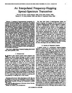
striking feature of relays is their low transmission power. Therefore power amplifiers they use are a lot cheaper than those of base stations (BSs). This fact also decreases the cost of the system. Relaying systems can be classified as amplify-and-forward or decode and forward [8]. In amplify-and-forward systems, relays amplify the received signal and then transmit it. They act as analog repeaters and therefore increase the noise level of the system, introduce the possibility of decoding error at the destination terminal, and experience delay due to signal propagation [9]. On the other hand, in decode-and-forward schemes, relays regenerate the received signal by fully decoding and re-encoding it before transmission. The relays act as digital repeaters, bridges or routers. In these systems, noise is not propagated along the channel. Decode-and-forward systems introduce decoding error possibility at the intermediate relays, and due to signal propagation as well as intermediate terminal decoding, they experience delay. In this thesis decode-and-forward relaying systems (digital relays) are used. Fig. 1-1 presents the system functional block diagram of a relay, BS and user equipment (UE) [10].
1.1 Thesis Motivation It is very important for today’s cellular systems to achieve high spectral efficiency in order to maintain their economical viability, since they require large quantities of scarce and increasingly expensive spectrum [11]. Therefore systems using the channel resources as efficiently as possible are becoming more attractive.
2
Relay
Note: UE can also receive directly from BS (not shown)
IP Packets Relayed Signaling
Buffer
C/I reported from UE (Relay to UE Link) When UE cannot reach Base Directly
Network Delay 1X1 Nomadic
MU
Channel Model
BS
L
L
Channel Model Relay Rx
Schedu ler
MU
1X1 Nomadic
BS Tx
L
UE
L Relay Tx
UE Rx
C/I measurement
C/I measurement
C/I Reporting Delay C/I Reporting Delay
DMUX
C/I reported from each relay (Base to Relay & Relay to UE Links) C/I reported from UE (Base to UE & Relay to UE Links)
TCP/IP Stack Application
Fig. 1-1 System functional block diagram of a relay, BS, and UE
3
The system proposed in this thesis assumes a broadband cellular mobile network with an aggressive channel reuse of 1. In order to deal with the striking interference problem
of
such
aggressive
channel
reuse
schemes,
certain
interference
management/avoidance techniques have been proposed [12]. These techniques require transmission coordination of BSs, which are interferers of each other. However, in the current wireless communications architecture neighboring BSs do no have a wired link between each other. Therefore, information exchange, hence transmission coordination cannot be done in a timely manner among BSs. Integrating relaying concept into conventional wireless communications systems increases high data rate coverage in a cost-effective manner while decreasing outage, among many benefits [1]. This thesis proposes a novel resource allocation scheme where frequency hopping is introduced into a relaying system. Recently AT&T and WINLAB proposed a new interference management technique, which is called Dynamic Frequency Hopping (DFH) [11]. DFH incorporates a non-traditional Dynamic Channel Allocation (DCA) scheme with slow frequency hopping (FH). The main objective is to provide capacity improvements through the addition of interference avoidance, which are higher than those provided by conventional frequency hopping, while preserving
interference averaging characteristics of
conventional frequency hopping in order to provide robustness to changes in interference [11]. Although DFH increases the performance compared to conventional systems as well as systems using random frequency hopping (RFH), it requires BS coordination.
4
Therefore, exploiting dynamic frequency hopping in current conventional wireless communications systems encounters the same practicality bottleneck described above. In cellular relay networks, BS and its relay stations (RSs) have a master-slave relation. In this architecture links between a BS and its RSs already exist. Therefore, interference management can be facilitated through transmission coordination in a cell. This thesis proposes a novel and practical interference management technique for cellular relay networks with very dense channel reuse.
1.2 Thesis Objectives This thesis proposes a system for downlink communications, where a broadband cellular mobile network with an aggressive channel reuse of 1 is assumed. The techniques proposed here can be applied to both of TDMA and OFDMA systems. Bearing this in mind, the objectives of the thesis can be summarized as follows: ! To introduce relays into Conventional Cellular Networks (CCN) exploiting adaptive modulation and coding. ! To increase the system performance, coverage and data rate, by averaging the interference using random frequency hopping (RFH). ! To improve the performance of the RFH-system by replacing RFH with dynamic frequency hopping (DFH) where, in addition to interference averaging, also interference avoidance is benefited from. ! To replace DFH with a novel concept, Dynamic Frequency Hopping with Limited Information (DFH-LI), which is proposed in this thesis, in order to maintain a
5
decentralized processing system, where (for resource planning issues) base stations of different cells do not need to communicate with each other. ! To determine the impact of relaying combined with various frequency hopping/management techniques on the system performance, such as average user spectral efficiency, outage probability and poor frequency hop ratio over the whole frequency hop pattern of a user.
1.3 Relevant Literature Multihop relaying has invoked great interest in the research community, which resulted in a number of publications focusing on various aspects of multihop relaying. It is shown in [13] that multihop concept is capable of providing significant high capacity cellular broadband radio coverage in 3G and Beyond 3G cellular wireless broadband systems. Focusing on fixed relays, [13] shows that the Quality of Service (QoS) of users which suffer a bad link with the BS because of heavy shadowing improves due to the deployment of fixed relay stations. In addition to improving radio coverage in cells with high shadowing, fixed relay stations also extend the radio range of BSs and enable them to provide service to much larger cells with broadband radio coverage compared to conventional single-hop cellular networks. [13] points out the need for additional radio resources for multihop systems since with the introduction of a RS, the BS-UE (user equipment) link breaks into BS-RS and RS-UE links, where different channels have to be used [1]. Therefore one crucial aspect of multihop wireless cellular networks is careful radio resource management. The work in [13] studies the
6
performance of multihop networks for three different concepts: Relaying in the time domain, relaying in the frequency domain and hybrid time-/frequency-domain relaying. A further research on multihop relaying focuses on load balancing [14]. By placing a number of ad hoc relay stations, the proposed iCAR system (integrated cellular and ad hoc relaying system) can efficiently balance traffic loads between cells. The idea behind this technique is to divert traffic from possibly congested cells to those with lower traffic. As a result, transmission power for UEs is reduced, system coverage is extended and system capacity is increased in an economical way. A novel and simple digital cellular infrastructure is proposed in [15], where seven RSs are deployed in strategic locations of the conventional cellular system, in order to increase throughput and coverage of the system. In this system, users do not communicate with preset RSs but they choose the best node (BS or RS) according to three criteria: pathloss, SINR or distance. In the proposed technique, instead of reserving extra channels for relay communication, the already used channels in the same cluster are assigned for UEs requiring relay assistance. Therefore no extra bandwidth is used. In this proposed pre-configured relaying channel selection algorithm, channel reuse is performed carefully in a controlled manner in order to keep the co-channel interference within acceptable levels. It is shown that without any loss of capacity the proposed technique increases throughput while decreasing outage, hence resulting in range extension [16]. Another multihop approach increasing throughput while decreasing outage is presented in [7, 17], and is called user cooperative diversity. This is a novel spatial diversity technique, where neighboring UEs cooperate and result in diversity gain. Results show that user mobility gives high spatial diversity advantages and outperforms a
7
non-diversity scenario. On the other hand, this approach also introduces some issues such as battery drain for UEs and security (users have direct access to each other’s data). Multihop channels with and without diversity for decoded and amplified relaying are discussed in [18], where also the mathematical modeling of these channels are investigated. The results show that the performance of multihop channels with diversity is always better than that of the channels without diversity. In addition, the amplified relaying multihop diversity channel outperforms the decoded relaying multihop diversity channel.
1.4 Thesis Organization This thesis is structured as follows: In Chapter 2, the important concepts of Dynamic Frequency Hopping (DFH) are introduced, which have been proposed by AT&T and WINLAB recently. Chapter 3 introduces several system models where relaying is combined with random frequency hopping (RFH), dynamic frequency hopping (DFH), and the proposed novel concept of this thesis, Dynamic Frequency Hopping with Limited Information (DFH-LI). Having described the simulation model for the performance analysis of these different systems in Chapter 4, the simulation results and their analysis are provided in Chapter 5. Finally, this thesis concludes with Chapter 6 which is devoted to summarize the key results of this research and to provide future research suggestions.
8
Chapter 2 - Dynamic Frequency Hopping Conventional frequency hopping is a means of implementing frequency diversity and interference averaging. The hop patterns can be determined randomly or cyclically. The fact that it is simple to implement and appropriate for providing robust communications links in interference limited and frequency selective channels makes Random Frequency Hopping (RFH) the most ubiquitous frequency hopping technique in commercial communications systems (e.g. GSM) [19-21]. For generic cellular systems, where frequency reuse of one is used, Wang, Kostic, and Maric [22, 23] have shown that implementing interference avoidance on top of frequency hopping can result in considerable capacity improvements. This fairly novel frequency hopping concept is called Dynamic Frequency hopping. The main idea of Dynamic Frequency Hopping (DFH) incorporates a non-traditional Dynamic Channel Allocation (DCA) scheme with slow frequency hopping (FH). The main objective is to provide capacity improvements through the addition of interference avoidance, which are higher than those provided by conventional frequency hopping, while preserving interference averaging characteristics of conventional frequency hopping in order to provide robustness to rapid changes in interference [11]. The key concept lying behind this intelligent frequency hopping technique is to adjust or create frequency hopping patterns based on interference measurements [24]. DFH uses slow frequency hopping and adaptively modifies the utilized FH pattern based on rapid frequency quality measurements. This technique combines traditional frequency hopping with DCA, where a channel is one frequency in a frequency hop pattern. The continuous modification of frequency hop patterns based on measurements represents an
9
application of DCA to slow frequency hopping. However, the fact that only some subset of frequencies in the whole FH pattern is replaced by a better quality subset makes this a non-traditional DCA scheme. The modifications are based on rapid interference measurements and calculations of the quality of frequencies used in a system by all mobiles and base stations (BS). The target of these modifications is tracking the dynamic behavior of the channel quality as well as of interference, and with the help of this information avoiding dominant interferers. DFH relies on continuous quality monitoring of all frequencies available in a system and modification of hopping patterns for each individual link. The measurements of all frequencies can be done in practice in traditional TDMA systems (at lower speeds) or in systems using orthogonal frequency division multiplexing (OFDM) [23].
2.1 How an Ideal DFH Method Works The first difference of DFH from conventional frequency hopping is in the way the patterns are built. Instead of using random (according to a PN code) or pre-defined repetitive hopping patterns (e.g. cyclic hopping sequences), in DFH the hopping patterns are generated for active users “on the fly”. With this new technique, the hopping patterns can be modified to adapt to interference changes. The length of the patterns is limited. The main idea behind creating the patterns is to choose the best frequency for each hop, which would correspond to the least interfered frequency. Hence, DFH requires continuous estimation and measurement of the interference at every frequency for every single hop of a pattern. At each hopping instant, the BS or the mobile terminal measures the quality of each frequency, filters the measurement to average out the instantaneous
10
Rayleigh fading effects, and then sends the data using the “best” frequencies chosen according to some quality criterion. For the sake of minimizing system instability and complexity, the number of hopping frequencies that change at every hop can be limited. The hopping patterns for users within the same cell are orthogonal at all times. The performance of a given link is monitored continuously by the BS; if this performance drops below a threshold, a better hopping pattern is generated. The only coordination for the BSs is that they are frame-synchronized with the BSs of the other cells. Therefore, the frequency hopping patterns of the users in a certain cell appear completely random to the users of different cells. The patterns can be updated in different ways. At this point, performance and complexity tradeoffs come into the picture. Three methods for FH pattern modifications are acknowledged: ! Full-Replacement Method ! Worst-Dwell Method ! SIR Threshold-Based Method
2.2 Full-Replacement Method In this method, all the frequencies used in a pattern are replaced with better ones in the next period. This method guarantees that during an entire transmission, frequencies with the best quality are used, provided that they are available. However, the fact that for all the available frequencies in the system rapid quality measurements (interference, SIR or other variables) is required, makes this method impractically complex. The reason for
11
the complexity is the large amount of data traffic between the BS and its users which is sent to modify the patterns. The FH pattern modifications are managed by the BS in a centralized fashion for all the mobile terminals communicating with this BS. Although this method gives the best possible performance of all DFH methods, because of the heavy messaging overhead it creates, this method cannot go further than being a theoretical case study indicating an upper limit of the performance. Fig. 2-1 simulates an example for pattern modifications performed according to Full-Replacement Method.
Pattern Modification
Frame 1 2
45
Hop 1
42
54
……
72
21
Frame 2 5
63
14
25
98
74
Hop 6
Fig. 2-1 Pattern modification for full-replacement method The best available frequencies in the first frame are replaced by the best available frequencies in the next time frame. The replacement of frequencies with the best available ones will occur even if using the frequencies of the first frame would have given a performance above the desired minimum quality threshold (e.g. SINR of the frame). In order to consider a possible application of DFH, more practical alternatives should be considered for pattern modifications where the decreasing complexity of these modifications will result in a decrease in the performance of the system. These reduced
12
complexity schemes limit how often and how much of a frequency hopping pattern may be modified. The following two hopping pattern modifications are of such suboptimal kind.
2.3 Worst-Dwell Method In order to reduce the messaging overhead, a satisfactory system performance may still be achieved by periodically changing only one (or an arbitrary number) of the frequencies in the pattern, which corresponds to the lowest quality (highest interference, lowest SIR, etc…) frequency of the pattern as shown in Fig. 2-2. Pattern Modification
Frame 1 2
45
42
54
72
21
Frame 2 2
45
65
54
72
21
Fig. 2-2 Pattern modifications for worst-dwell method At every frame a specified number of frequencies (in the example above, only one frequency) are updated. This does not mean that the performance in all the rest of the frequencies is perfect. There might be a situation where the performance suffers beyond the quality threshold for more than one frequency. Still, only the frequency with the worst performance is replaced, since the example only allows modifying only one frequency at each period. 2.4 SIR Threshold-Based Method As the previous method, this method also has a messaging overhead less than that of Full-Replacement method. The pattern updates are done sparingly instead of
13
periodically. Based on SIR measurements on the frequencies of a pattern, the current hopping pattern is changed if the measured SIR is below a required threshold on at least one of the frequencies. Instead of replacing all the frequencies as was the case in the FullReplacement method, only this low quality frequency (or frequencies) is replaced with a new one. This frequency can be replaced by any frequency meeting the threshold SIR. Therefore, there is no need for all the frequencies to be scanned (to find the best one), which reduces the overhead. Another factor reducing the messaging overhead is that the frequency updates are performed whenever necessary instead of periodically. Frame 1 2
45
42
54
Frame 2 72
21
2
No Modification
45
42
86
72
35
Frame 3 2
45
42
86
72
35
Fig. 2-3 Pattern modifications for SINR-Threshold method
After the quality measurements and calculations in the first frame, it is found out that the SINR at the fourth and sixth hop is below the previously specified threshold SINR. Therefore, the frequencies in these hops are replaced with some frequencies which satisfy a SINR level above the threshold. There is no need to go through all the available frequencies. The search is not for the best frequency but for any frequency that results in sufficient SINR.
14
Proceeding the same way also in the second frame, the results show that all six frequencies satisfy the SINR condition. It is important to note that there is no information hidden in these results regarding whether these six frequencies are the best ones or not. Since these six frequencies satisfy the SINR condition, no measurements are performed on the quality of the other available frequencies, which reduces the signaling overhead, hence the complexity of the system. Next we will present two different kinds of Dynamic Frequency Hopping methods proposed in the literature: “Measurement Based DFH” and “DFH with Network Assisted Resource Allocation (DFH with NARA)”. The first model is a theoretical one, whereas the second one is appropriate for practical systems.
2.5 Measurement-Based Dynamic Frequency Hopping This is an ideal theoretical DFH scheme. It introduces the original idea of DFH [24]. Straightforward Measurement-Based DFH is implemented in the following way for the downlink: i.
Each mobile continuously measures the quality of all frequencies available in the system (signal strength, interference, SIR, or other criteria).
ii.
The measurements are communicated over the air to the serving BS.
iii.
Each BS collects the interference measurements from all of its mobiles.
iv.
Based on the measurements, the BS periodically updates frequency hop patterns for the mobile stations, such that the overall performance is optimized.
v.
The BS sends information to each individual mobile informing it of the frequency hop pattern that will be used in the ensuing time period, as shown in Fig. 2-4.
15
PUE-6
f 11
f 32
f 28
f 13
f02
f 46
f49
PUE-1
PUE-5
f25
f53
f67
PUE-4
f61
f48
f35
f63
PUE-3
f63
f19
PUE-2 f53
f15
f03
f65
f21
f67
f59
f17
f17
f07
f50
f05
f39
f01
f27
f61
f41
f15
f02
f27
Base Station
User Equipment
PUE-i
Pattern assigned to UE-I by the BS
Fig. 2-4 Each BS assigns future patterns to its UEs
16
Similar processes can also be done for the uplink, although the primary concern of this thesis is the downlink. In order for the BS to be able to assign frequency hopping patterns according to a certain quality criterion (such as SINR), it needs to know how the quality of the links between itself and every single UE at each frequency at each frequency hop in the next frame is. After collecting the information from its mobiles, the BS knows exactly how the transmission quality of a certain frequency in the next time frame at a certain time slot will be. After having this information, the BS can compare these quality measures with the quality requirements of the cell and then modify these patterns according to the three different pattern modification methods described previously. Therefore, its future FH pattern-time slot assignment is totally based on this information.
2.6 Dynamic Frequency Hopping With Network Assisted Resource Allocation (DFH with NARA) Measurement-based DFH is only a theoretical model and needs modifications in order to be able to be used efficiently in real life. Two main practical problems are: ! The need to perform rapid interference measurements at all relevant frequencies, both at the mobiles and the BS. ! The signaling overhead required communicating the measurement results to the BS. Using real time inter-base signaling for intercell interference management and taking advantage of frame synchronization on a system level, NARA finds a solution for
17
these bottlenecks. Its striking feature is that it benefits from frame synchronization on a system level and provides functionality identical to that of the measurement- based DFH. The following figure is the illustration of the system structure, where NARA is exploited for downlink DFH management:
MOBILE STATION Measure Pathloss on BCCH for BS 1
…….
Measure Pathloss on BCCH for BS K
Average
…….
Average
…….
Send to BS1
Send to BS1
Read and Use Specified FH Pattern
WIRELESS MEDIUM From Other Mobiles
To Other Mobiles
BASE STATION Collect Measurements From All MS in this BS Coverage Area
Local Copy of Measurements For All MS from
Manage Frequency Hop Patterns For This BS
Send Orders To MSs with Next FH
Local Copy of FH Patterns For All BS
From Other Base Stations From Other Base Stations To Other Base Stations
To Other Base Stations
LANDLINE NETWORK
Fig. 2-5 Block diagram of a cellular system that supports DFH (downlink) [24]
18
In the following, BS-autonomous frequency hopping pattern assignment is assumed. However, a centralized management is also possible. Focusing on the block diagram above, it is noticed that: ! Each mobile continuously measures path losses (only) to all BSs in its neighborhood ! These measurements are sent through a low-pass filter to average out instantaneous Rayleigh fading effects ! The mobile sends the measurements to its serving BS over wireless link The measurement reporting rate in DFH with NARA need not be very high, e.g., the rate used for Mobile Assisted Handoff would be enough. In [24] this rate is specified as 2 sec. With this rate, the system combats only against shadowing and not multipath fading. If multipath fading were taking into account, the reporting rate should be considerably higher than this, which would increase the messaging overhead. The methods used and proposed in this thesis also assume low measurement reporting rates and combats only against shadowing. In the mean time, the BSs exchange the measurements reported from their own cells. Thereby, all the BSs have access to the path loss, FH pattern, channel assignment and transmit power level information for the active links of the neighboring mobiles, which are the main interferers for their own links. Therefore, BSs use this information to manage their intelligent dynamic frequency hopping patterns, and execute interference avoidance. This is the main practicality of DFH with NARA compared to the Measurement-Based DFH. The rapid quality measurements of all available frequencies at
19
all available time slots performed by each UE is replaced by the computation of interference conditions by BSs, which use this exchange data. The technique used to generate the hopping patterns is Least-Interference-Based DFH with NARA, which is appropriate for a TDMA system. In this technique, a resource is defined as a time slot and a frequency hop pattern used in that slot. 2.6.1 How the System Works The system works in the following way: ! Each terminal measures path losses to the neighboring BSs and transmits this information to its serving BS on a regular basis.
Base Station User Equipment
Fig. 2-6 Measurement-based DFH for downlink Each mobile continuously measures the quality of all frequencies available
20
! Each BS communicates to several tiers of its neighbors the information about its own resource utilization: time slots, frequency hopping patterns, and power levels that are currently in use (Fig. 2-7).
Base Station
User Equipment
Fig. 2-7 Least interference based DFH with NARA
21
Note: For this particular algorithm, it is not necessary for the BSs to exchange any path loss information of active links, but they exchange their resource utilization information (i.e. which frequencies will be used by their UEs at what time slot, and what is the transmission power of the BSs). However, for the sake of capacity improvement, more complex algorithms could take advantage of sharing this information. ! Combining the information received from other BSs regarding to their own resource utilization and the path loss measurements reported by its terminals, the serving BS calculates the interference level at each available resource, determines the least-interfered time slot and FH pattern pair, and assigns this to the terminal. For a specific resource (time slot FH pair), the interference by other BSs is PInt = PRx = PTx –PL,
(1)
where PTx is the power transmitted by interfering BSs, PL is the path loss of neighboring (interfering) BSs to the UEs of the serving BS. The UEs measure this pathloss based on the BS pilots. With this information, the serving BS can easily calculate the interference power at a particular resource. It is important to note that the mobiles are not assigned a pre-defined pattern (such as pseudo random or cyclic hopping patterns). The hopping sequence is generated by the BS dynamically according to the interference level on each frequency at each hop. ! This procedure applies to new as well as to currently active users, the serving BS continuously monitors each user’s performance and reassigns it another resource if the performance degrades below a threshold.
22
A staggered-frame resource management can be used to avoid the problem of two nearby BSs assigning at the same time the same good frequencies for future FH patterns of their users. In a cellular system, the staggered frame concept would work in the following fashion: i.
BSs are frame and superframe synchronized;
ii.
control reuse pattern is defined in time, according to which only one BS is allowed to change frequency hop patterns for the duration of one frame;
iii.
all BSs get an opportunity to modify frequency hop patterns of their mobiles once per superframe.
An
example
for
the
staggered
frame
concept
is
shown
in
Fig.
2-8:
23
Frame 1
Frame 2
Frame 3
Frame 4
Frame M
BS-1 f11 f32 f28 f13 f46 f02 f11 f32 f28 f13 f46 f02 f11 f32 f62 f13 f46 f02 f11 f32 f28 f13 f46 f02 … f11 f32 f28 f13 f46 f02
BS-2 f53 f50 f39 f01 f27 f61 f53 f50 f39 f01 f27 f61 f53 f50 f39 f01 f27 f61 f53 f50 f39 f01 f27 f61 … f44 f50 f39 f01 f27 f61
BS-3 f25 f53 f67 f61 f35 f15 f25 f22 f67 f61 f35 f19 f25 f53 f67 f61 f35 f15 f25 f53 f67 f61 f35 f15 … f25 f53 f67 f61 f35 f15
. . .
. . .
. . .
. . .
. . .
BS-N f63 f67 f17 f15 f02 f27 f63 f67 f17 f15 f02 f27 f63 f67 f17 f15 f02 f27 f30 f33 f17 f09 f20 f27 … f63 f67 f17 f15 f02 f27
Superframe Fig. 2-8 Superframe Concept (frequencies in bold-italic font are the modified new frequencies). Note that in each frame, only one BS modifies its frequencies
24
Chapter 3 - Two-Hop Wireless Cellular Networks With Random Frequency Hopping (RFH) and Dynamic Frequency Hopping (DFH) This thesis focuses on a novel idea for Cellular Relay Networks: dynamic frequency hopping with limited information. The proposed system architecture is given in Fig. 3-1. Due to the fact that downlink (DL) communication requires much higher speeds than uplink (UL), only downlink will be examined. In the future UL speeds will increase as well, however, there’s still going to be an asymmetry in speed towards DL. Therefore there is a bigger need to increase the performance of DL. The proposed two-hop cellular system is composed of one BS and six RSs placed uniformly around the BS. The RSs are deployed in the cell such that they can support a good link with the BS (most preferably at line-of-sight locations). Because of these RSs, each cell consists of seven neighborhoods, called sub-cells. Six of these sub-cells correspond to the RS neighborhoods and these sub-cells surround the BS neighborhood, which is the seventh and the center sub-cell. The frequency reuse in a neighborhood in a cell is one. This means that at a specific time the same frequency can be used seven times in a cell (since a cell consists of seven sub-cells or neighborhoods). The patterns assigned to UEs in a sub-cell are orthogonal to each other. Hence, there is no in-subcell interference. It is also assumed that there is no adjacent channel interference either. The only existing interference experienced by the UE is out-of-subcell interference created by the RSs and/or BSs of the surrounding sub-cells. The BS – RS link is very important for the speed and quality of the whole system’s communication. A RS serves to a number of user equipments. The active
25
UEs in the RS neighborhood, which get the strongest signal from a RS*, communicate all their data through the RSs.
Base Station Relay Station User Equipment Cell Border Relay or Base Neighborhood
Fig. 3-1 System architecture for the proposed relay system
Relay-Base Communication through Directional Antennas
*
Note that although being in a certain RS neighborhood, due to shadowing, the strongest signal picked by the UE might originate directly from the BS or even from neighboring RSs
26
Having collected the data of several UEs, the RS sends this data to the BS. Then on the downlink the BS sends all the data, which is directed to the UEs in RS neighborhoods, to the RSs. Hence, compared to the RS-UE or UE-BS link, the RS-BS link carries much more information and increasing the quality of this link increases the speed and the quality of the whole system. Therefore, six directional antennas are deployed between the BS and the RSs (one directional antenna for each RS-BS link). In addition to this, to communicate with the UEs, the BS and the six RSs use omnidirectional antennas. As a result, the BS is deployed with seven antennas. UEs also use omni-directional antennas for communicating with the base as well as with the RSs. In this proposed system, the BS has two modes for the transmit power: ! High Mode: The transmit power is 20 W; ! Low Mode: The transmit power equals the RS transmit power (3 W) The RS transmit power is kept lower than the BS high power mode and equal to the low power mode (3 W). It is crucial that the BS power is allowed to be high enough to be the dominant power in the whole cell (being considerably higher than the RS transmit power). The reason for that is the support of the control and signaling functions. These functions are needed for the BS to be able keep track of the UEs all over the cell. In the case of letting the BS operate in the low power mode only, since there will not be a dominant power entity throughout the whole cell, these functions need to be moved to the RSs (a UE which is far from the BS, receiving a very good signal from its RS cannot be tracked by the low power center BS but the serving RS only). This scheme would complicate the RS design, and would increase their cost and complexity to that of a microcell. However, one of the main advantages of the RS and multihop technology is
27
that the RSs are very simple, physically small, technically easily implemented devices, and hence considerably cheaper than BSs; this makes RSs more attractive to deploy. Therefore, in order to increase coverage and the quality of the communication, a high number of RSs can be added to the cell. Hence, it is in the best interest that they are kept simpler than the BSs. In addition, passing the control and signaling functions to the RSs will introduce new technical problems, which need to be looked into thoroughly, and will not be considered in this thesis. Since the BS is operating in two different transmit power modes, a Time Division Multiplex (TDM) scheme is used, where the time is divided into two time slots. Since different functions are active in these time slots, they also have different lengths.
3.1 Time Slot 1 In this time slot, the BS transmits with high power (20 W). It sends data to RSs while sending control and signaling messages to UEs, which requires the high power mode to reach the UEs at the periphery of the cell as well. RSs cannot transmit and receive at the same frequency [1]. The reason for this is the positive feedback of the transmitting end at the receiving end of the RS. The transmission power is a lot higher than the receiver power of the RS. Since the RSs cannot receive and transmit at the same time, the transmission and reception functionalities are also divided into different time slots for the RSs. A decision should be made regarding which function of the RS should be active in this time slot.
28
Since downlink communication is considered, transmission for a RS means transmitting data to the UEs. On the other hand, if a RS receives a signal, this has to be originated from the BS. When the BS serves in low power (which is described in the next time slot), it is only responsible of its own small neighborhood (the center sub-cell). This power is not enough for the BS to support a good link with the RSs. Additionally, letting the RSs transmit data to the users in their neighborhood while the BS is transmitting at high power, will cause very severe interference for the RS-UE communication. Therefore, it is of the best interest that the RSs do not transmit but only receive from the BSs. Besides BS-RS link, also the BS-UE link has to be considered. While the BS is transmitting with high power and no RS is transmitting (hence the BS being the dominant power source in the whole cell), there are three possibilities for the link between the base and the UEs: ! BS transmits data to the mobiles which are in its neighborhood only ! BS transmits data to all the UEs in the cell. UEs communicating with RSs in the next time slot will get the same information twice, since the BS is sending the same information to the RSs, too, so that the RSs can pass this information to their UEs in the next time slot. This option results in diversity potentials ! BS does not transmit data to the UEs at all; this results in easy resource management. However, if there are very good BS-UE links (e.g. 64-QAM) with the UEs in the RS neighborhood, these links are wasted or ignored. Assuming that the number of these good links will be small compared to the rest of the BS-UE
29
links (especially with the increasing number of users in the system), it is reasonable to ignore these links.
This thesis assumes that in the first time slot the BS does not transmit data to any UE. The third type of communication in this time slot is the control and signaling functions of the BS used in order to keep track of the RSs as well as UEs. These signals sent by the BS do not interfere with the data communication signals above, since the channels used for data communication and control/signaling functions are orthogonal to each other. Therefore, there is no need to worry about these signals when dealing with resource management. Communication in this time slot includes the FH patterns sent to the RSs by the BS, which will be passed to the UEs in the next time slot. It is possible that there might be some imperfections in the first time slot. Any imperfection would result in UEs using non-optimal FH patterns, which would result in a degradation of the system performance. However, the system is designed to minimize the possibility of imperfections. RSs are deployed at locations where they have a line-of-sight (LOS) with the serving BS. On top of that, there is a directional antenna between each RS and its serving BS. In this time slot, BSs transmit with high power. In order to combat imperfections, low rate error control coding (ECC) schemes can be applied. Therefore it is reasonable to assume that in this time slot the RS-BS link is perfect for all practical purposes. A summary of the functions active in the first time slot is shown in Fig. 3-2.
30
Base Station Relay Station UE BS-RS Data Link BS-UE ControlSignaling Link
Fig. 3-2 Communication in the first time slot 3.2 Time Slot 2 In the second time slot, the BS transmits at low power, which is equal to the transmission power of the RSs, while the RS transmission power is a parameter. Therefore, there exists no dominant power source throughout the whole system. In this time slot, the RSs do not receive from the BS, but they only transmit to the UEs in their coverage region (which ideally overlap with their sub-cell neighborhood). Due to shadowing, it is also likely that a UE which is located in a certain RS’s neighborhood might pick up a signal from a different RS or from the center BS, which is stronger than
31
the closest RS’s power. In this case, although being closer to one RS, the UE might communicate with a power source further away in the cell. Meanwhile, the BS transmits data to the UEs which are in its coverage region only. The seven coverage regions for the BS and the surrounding six RSs are of the same size, since the transmission power of the BS equals that of the RSs in this time slot. Fig. 3-3 summarizes the communication in the second time slot.
Fig. 3-3 Communication in the second time slot In a conventional cellular system, considering downlink, the users get interference from other cells. If no frequency hopping is used, a certain UE will always get interference at the same frequency from the same BS. If this interference level is low, the quality of the communication for this user will be satisfying all the time. On the other hand, if the user is getting severe interference from a certain BS, then it will experience outage. In this proposed cellular relay network architecture, the interference to a UE in a certain neighborhood will come from the surrounding RSs and/or BS of the cell in the first and second tier around this neighborhood. Note that some of these interferers are
32
out-of-cell interferers (RSs of other cells). Fig. 3-4 shows the first tier and second tier interferers.
First Tier Interferers Second Tier Interferers Base Station Relay Station User Equipment Cell Border Relay or Base Neighborhood
Fig. 3-4 First and second tier interferers for a selected relay station Before analyzing DFH-LI, a random frequency hopping RS system will be investigated as a reference system.
3.3 Random Frequency Hopping With Varying Cyclic Shifts In Cellular Relay Networks Assuming an interference limited system, frequency diversity and interference averaging can be achieved by exploiting RFH. RFH is simple to implement and suitable for providing robust communication links in such systems. Therefore, RFH brings up the
33
performance of UEs with poor quality links to an average quality level, while bringing down the performance of UEs communicating on high quality links again to this average. Since the performance of the bottleneck users has improved, there are less users experiencing outage, whereas also the number of UEs experiencing high quality communication decreases thereby. The RFH patterns are specified in a cyclical fashion, as Fig. 3-5 shows. If there are N channels or frequencies (in this research these notions will be used interchangeably as explained in the Dynamic Frequency Hopping section of the thesis), there can be at most N orthogonal frequency hopping patterns. This feature prevents any interference coming from inside of a certain neighborhood; UEs in a neighborhood do not interfere with the other UEs in the same neighborhood. The same frequencies will be available in the neighboring RSs and BSs, too, because of the frequency reuse being one. If two users in neighboring sub-cells use the same patterns, they will interfere with each other at each frequency hop throughout the whole operation. The interference will be experienced at different frequencies but from the same source. Therefore, the idea of frequency hopping loses its significance. The difference between hopping and no hopping vanishes as choosing the same pattern results in continuous interference for two UEs as if there was no frequency hopping, and two UEs are communicating with their RS or BS using the same single channel.
34
P0:
0
3
6
9
2
5
8
1
4
7
P1:
1
4
7
0
3
6
9
2
5
8
P2:
2
5
8
1
4
7
0
3
6
9
P3:
3
6
9
2
5
8
1
4
7
0
P4:
4
7
0
3
6
9
2
5
8
1
P5:
5
8
1
4
7
0
3
6
9
2
P6:
6
9
2
5
8
1
4
7
0
3
P7:
7
0
3
6
9
2
5
8
1
4
P8:
8
1
4
7
0
3
6
9
2
5
P9:
9
2
5
8
1
4
7
0
3
6
Fig. 3-5 FH pattern creation In order to prevent such a scenario, the same frequencies with different patterns can be used in different sub-cells. These patterns can be designed so that the effects of a possible interference situation can be minimized. When designing the patterns in cyclical fashion, using a different cyclical shift for each sub-cell which can cause interference for each other, increases the level of interference averaging and frequency diversity. If for interference calculations only the first and second tier RSs and BSs are considered, this
35
model makes sure that the same cyclical shift will not be reused in these tiers. This idea is illustrated in Fig. 3-6. Assume that the interference experienced by sub-cell-1 is investigated, where subcell-2 to sub-cell-4 are the interferers. Sub-cell-1 will assign to its UE one of the patterns P1,11 through P1,10. The same process will be done in the other sub-cells, too. The number of the patterns assigned depends on the loading of the system, where with loading we refer to the ratio of the number of users in the cell to the total number of available channels. If the loading is 0.7 and there are 10 available channels in a cell, then the cell will use seven of its patterns. If sub-cell-1 assigns P1,3 to its UE, in the first frequency hop the interfering patterns from will be P2,3, P3,3, and P4,3 (if they are assigned by the BS to a UE). In the second hop, the interferers will be P2,1, P3,7 and P4,5 (If they are assigned by the BS to a UE).
1
The notation Pi,j refers to the jth pattern of the ith sub-cell.
36
Sub-Cell: 1, Shift: 1
Sub-Cell: 2, Shift: 3
P1,1:
1
2
3
…..
9
10
P2,1:
1
4
7
…..
5
8
P1,2:
2
3
4
…..
10
1
P2,2:
2
5
8
…..
6
9
P1,3:
3
4
5
…..
1
2
P2,3:
3
6
9
…..
7
10
. . .
. . .
P1,9:
9
10
1
…..
7
8
P2,9:
9
2
5
…..
3
6
P1,10:
10
1
2
…..
8
9
P2,10:
10
3
6
…..
4
7
Sub-Cell: 3, Shift: 7
Sub-Cell: 4, Shift: 9
P3,1:
1
8
5
…..
7
4
P4,1:
1
10
9
…..
3
2
P3,2:
2
9
6
…..
8
5
P4,2:
2
1
10
…..
4
3
P3,3:
3
10
7
…..
9
6
P4,3:
3
2
1
…..
5
4
. . .
. . .
P3,9:
9
6
3
…..
5
2
P4,9:
9
8
7
…..
1
10
P3,10:
10
7
4
…..
6
3
P4,10:
10
9
8
…..
2
1
Fig. 3-6 Frequency patterns in neighboring sub-cells. In order to decrease interference, neighboring sub-cells use different shifts while creating patterns; hence same patterns will not be used in the neighboring sub-cells
37
3.3.1 How to Choose the Cyclical Shift The cyclical parameter should not be a dividend of the total channel number, otherwise, only certain frequencies will be used. As an example, assume that the total number of channels is 40. If the cyclical shift is 20, then the pattern will be 20-40-20-40 etc., which is not a preferred situation. Choosing the cyclical shift as an even number requires special care. If the total channel number is an even number, too, then depending on the beginning frequency of the pattern either even or odd frequencies will be ignored (if the beginning frequency is an even number, then the whole pattern will exist of even numbers, vice versa). For a system with a total of 18 channels and a cyclical shift of 4 the patterns will look like as follows: 2-6-10-14-18-4-8-12-16-2-6… where the odd numbers are ignored or 3-7-11-15-1-5-9-13-17-3-7… where the even numbers are ignored. On the other hand, if the total number of the channels in the system is an odd number, the cyclical shift being an even number, all the frequencies will be used in the patterns. For 13 channels and a cyclical shift of 4 the patterns will look like as follows: 7-11-2-6-10-1-5-9-13-4-8-12-3-7-11… 6-10-1-5-9-13-4-8-12-3-7-11-2-6-10… If the cyclical shift is an odd number, provided that it is not a dividend of the total number of channels, there is no problem; i.e. all the frequencies are used in a pattern. The following proposed system of the thesis combines RFH and DFH in such a way, that the future interference is predicted as much as it can be, while keeping the whole system and all the processes as decentralized as possible.
38
3.4 Dynamic Frequency Hopping With Limited Information (DFH-LI) In this technique to utilize the resources in the second time slot, the basic principles of Dynamic Frequency Hopping (DFH) are used. DFH combines the advantages of both dynamic resource allocation (interference avoidance), and of frequency hopping (frequency diversity) [11]. FH will help in minimizing the effect of interference on the performance. The hopping patterns are going to be generated for active users on the fly, according to some measurements and calculations performed in real-time; i.e. there is no pre-defined FH pattern such as pseudo-random patterns, cyclic patterns, etc. The following two cases are investigated: i.
BS- UE communication
ii.
RS – UE communication In the second time slot, neither the BS nor the RSs perform control and signaling
functions. In the analysis below, only the first tier of transmitters (RSs and/or BSs) will be considered as interferers. The analysis for two tiers of interferers is similar.
3.4.1 BS – UE Communication The BS will assign a frequency hop (FH) pattern to its users in its neighborhood. The serving BS should do this assignment according to a performance criterion such the SINR2 value etc. During pattern updates, the defective frequencies with a SINR level
2
In the original DFH described in Chapter 2, the performance criterion is SIR, whereas in our proposed system we use SINR.
39
below the threshold SINR will be replaced with the frequencies supporting SINR levels above the threshold. The crucial information the BS needs is the interference at the UE in a certain time slot with a certain FH pattern. The potential interferers are the six RS surrounding the BS. In order for the BS to calculate the interference caused by these RSs at the UE, the BS needs to know: i.
Transmit power of the RSs
ii.
Resource utilization information of the RSs
iii.
Pathloss of the RSs to the UE Since in the first time slot the BS has assigned the resources to the RSs, and since
the RSs have a constant transmission power, the BS already has the information i) and ii). The third piece of information comes from the UEs. Each UE measures the pathloss to the neighboring RSs and reports this information to its serving BS (Fig. 3-7).
40
Fig. 3-7 Pathloss measurements Having collected this information, the BS calculates the interference level at each available resource, determines the least interfered time slot and FH pattern pair, and assigns this to the UE. After this, the BS continuously monitors each user’s performance and reassigns another resource if the performance (SIR in this case) degrades below the threshold SIR. The system block diagram is shown in Fig. 3-8.
3.4.2 RS – UE Communication In the case of the RS communicating with one of its UEs, there are again six potential interferers: the serving BS of the cell, two RSs from the same cell and three RSs from different cells. The serving BS will assign the resources to the UE (Fig. 3-9).
41
In this thesis a decentralized system is assumed, where communication and data transfer between different cells is minimized. Since three of the interferers are in different cells, DFH, as proposed in [11], would require BSs of different cells to communicate with each other. UEs perform pathloss measurements to the two in-cell RSs and the BS, and send it to their RS. The RS passes this information to its serving BS. According to DFH, all the interferers need to report their transmission power level and resource utilization information (which FH pattern they are using in which time slot and at which power) to the BS which is going to assign resources for the UE [24]. However, the two in-cell RSs do not need to report their resource utilization information to the BS since from the previous time slot the BS has this resource utilization information (in the first time slot the BS determines which resources the RSs are going to use, and it keeps this information
42
CASE-1: UE in BS-Neighborhood UE Measure Pathloss for RS1
…
Measure Pathloss for RS6
Average out Rayleigh
…
Average out Rayleigh
Get the new FH Pattern
BASE STATION Notify UEs in BS Neighborhood with their new FH Patterns
UEs IN BS NEIGHBORHOOD
Store FH Patterns of all UEs and RSs in Memory
Collect Pathloss Reports from UEs in BS Neighborhood
Create new FH Patterns for UEs in BS Neighborhood
NO COORDINATION
LANDLINE NETWORK
IN-CELL RELAYS
OUT-OFCELL RELAYS
OTHER BASE STATIONS
Fig. 3-8 Block diagram for a user in BS neighborhood in the second time slot of a DFH-LI system
43
for the calculations in the second time slot). Thereby the serving BS has the necessary information for R1 as well as its in-cell interferers. However, there is no communication between the three RSs in the other cells and the serving BS.
R2 R3 R1
BS
R4 R6 R5
Fig. 3-9 RS – UE communication. R1 passes the pathloss information of the UE to the BS, since BS is in charge of resource assignments of the UEs The serving BS knows in a certain time slot for sure, at which frequencies the SIR is below the threshold value, so it does not assign these frequencies to the UE. These frequencies are blocked for that very frequency hop. This part is DFH. However, since the BS is missing necessary interference information from other three outer-cell RSs, it
44
does not know the quality level at different frequencies in that hop. Therefore, it can assign any of the frequencies, which is not blocked by the DFH part of the FH scheme. However, there is no guarantee that the quality of service (QoS) will be acceptable at that frequency. BS has no idea if the out-of-cell interfering RSs are using the frequencies that according to the results and calculations of the DFH part satisfy an SIR level above the threshold and are not blocked. Therefore, this proposed technique is called DFH with Limited Information. Fig. 3-10 shows the corresponding system block diagram when a user is in a RS neighborhood. For comparison purposes the original block diagram of DFH with Network Assisted Resource Allocation (DFH with NARA) is shown in Fig. 3-11 again.
45
CASE-2: UE in RS-Neighborhoods UE Measure Pathloss for BS
Average out Rayleigh
Measure Pathloss for Interfering Relay1
Average out Rayleigh
Measure Pathloss for Interfering Relay2
Average out Rayleigh
Get the new FH Pattern
BASE STATION
UEs IN RS NEIGHBORHOODS
Notify RSs with the new FH Patterns for UEs in RS Neighborhoods
Store FH Patterns of all UEs and RSs in Memory
Collect Pathloss Reports from UEs in RS Neighborhood
Create new Random FH Patterns for UEs in RS Neighborhoods from the pool of available and unblocked resources
Calculate which resources result in a SIR less than the threshold SIR, SIRTh, and block them
NO COORDINATION Notify UEs in RS Neighborhoods with their new FH Patterns
IN-CELL RELAYS
LANDLINE NETWORK Get the new FH Pattern OUT-OFCELL RELAYS
OTHER BASE STATIONS
Fig. 3-10 Block diagram for a User in RS neighborhood in the second time slot of a DFH-LI System
46
MOBILE STATION 1 Measure Pathloss on BCCH for BS 1
…….
Average
…….
Send to BS1
…….
Measure Pathloss on BCCH for BS K
Average
Read and Use Specified FH Pattern
Send to BS1
WIRELESS MEDIUM From Other Mobiles
To Other Mobiles
BASE STATION Collect Measurements From All MS in this BS Coverage Area Local Copy of Measurements For All MS from All BS
Manage Frequency Hop Patterns For This BS
Send Orders To MSs with Next FH Patterns
Local Copy of FH Patterns For All BS
From Other Base Stations From Other Base Stations To Other Base Stations
To Other Base Stations
LANDLINE NETWORK
Fig. 3-11 Block diagram of a cellular system that supports DFH with NARA (downlink)
47
Chapter 4 - Simulation Model 4.1 Propagation Model Being unpredictable and random, wireless communications radio channels are one of the elemental limitations on the performance of the systems [25]. In order to simulate the radio channel as real as possible, mobile radio system designers have come up with various propagation models such as Okumura, Hata, and COST-231, where reflection, diffraction and scattering effects were taken into account. In this thesis the following fairly simple propagation model is used [25]: Pr = Pt
G Xσ PL
(2)
where Pr and Pt are the received and transmit powers, respectively. G is defined as the combined antenna gain of the receiver and transmitter, where G = GrGt.
(3)
X σ is a zero-mean Gaussian distributed random variable (in dB) with standard deviation of σ (in dB) representing the lognormal shadowing. Finally, PL is the average pathloss, which is given by 2
n
4πd 0 f d PL = , c d0
(4)
where d0 is the close-in reference distance, determined from measurements close to the transmitter, f is the carrier frequency, c is the speed of light (c=3.0x10⁸ m/s), d the distance between the transmitter and the receiver, and at last, n is the propagation exponent.
48
4.2 Environment and Parameter Assumptions
In this section, a list of the parameters used in the simulations of this research is presented. This data is widely used in cellular networks simulations [15]. ! Pathloss propagation exponent, n = 3.5 ! Lognormal shadowing with 0-dB mean and 8-dB standard deviation ! Multipath fading is not taken into account ! Simulation area (for three different types of networks) is shown in Fig. 4-1. These
networks will be described in more detail later in this chapter. ! RF Carrier = 2 GHz ! Transmission Bandwidth, W = 1 MHz (narrowband) and 50 MHz (broadband) ! Thermal noise with a noise figure, F = 8dB ! Isotropic antennas with unit gain (for BSs, RSs and UEs) ! Power control is not used ! BS transmit power = 20W (high) and 3 W (low) ! RS transmit power = 3W ! Downlink only
These parameters are valid for the BS-UE and RS-UE links. It is assumed in the simulations that the BS-RS can effort the highest adaptive modulation and coding (AMC) mode with negligible errors.
49
2R
R
Base Station Relay Station Cell Border Relay or Base Neighborhood
CCN
CRN
Fig. 4-1 Simulation areas for conventional cellular networks (CCN) and cellular relay networks (CRN), where R = 300m 4.3 Adaptive Modulation and Coding (AMC)
Adapting the transmission power and modulation to the environment and instantaneous propagation conditions, interference scenarios and traffic or data rate conditions, higher spectral efficiency and yet flexible data rate access can be satisfied. [26]. Using this technique, which is called adaptive modulation, even without exploiting power control, a significant throughput advantage is gained. In this thesis, AMC is performed using the combinations of QPSK, 16-QAM and 64-QAM, and five code rates (1/2, 2/3, 3/4, 7/8 and 1). As the coding scheme, Bit Interleaved Coded Modulation (BICM) is exploited. The following graph shows the bit error rate (BER) versus SINR behavior for various combinations (Fig. 4-2). Specifying the target BER as 10-5, Table 4-1 presents for each combination the required SINR and spectral efficiency, which would satisfy the BER criteria of 10-5.
50
Fig. 4-2 BER vs. SINR for combinations of various modulations and code rates*
*
The data used to generate this figure is given in Table 4-1 and provided by Dr. Sirikiat Lek Ariyavisitakul.
51
Table 4-1 Relation of all combinations, required SINR and spectral efficiency that will yield BER of 10-5 This thesis does not consider any physical layer (PHY-Layer) issues. This lookup table is the interface to the PHY-Layer. SINR for a user is calculated and then the corresponding spectral efficiency of the user is specified from this table.
52
4.4 Simulation Algorithm
Simulations are performed for two different systems and their performance is compared. These systems are: ! Conventional Cellular Networks (CCN) ! Cellular Relay Networks (CRN)
After giving the system descriptions for these networks, several simulations will be performed and their results will be discussed in the next chapter.
4.4.1 Conventional Cellular Networks (CCN)
The system architecture for CCN consists of seven cells, where one center cell is surrounded by six others, as shown in Fig. 4-3. The BSs transmit at a power of 20 W. This system will be used for comparison purposes and will be the lowest performance system. The techniques investigated in this thesis for relay systems will be also applied to CCN and any gain or degradation in performance will be specified.
4.4.2 Cellular Relay Networks (CRN)
The system architecture used for the simulation of CRN consists of seven cells again, which have the same size as the ones in CCN. The difference is, however, that in this case each cell has six RSs, as shown in Fig. 4-4. As described in the previous chapter, the relay stations in a cell communicate with their BSs via directional antennas. Therefore, in the simulations, this link, which is being used in the first time slot, is considered to be perfect. Hence, only the second time slot is simulated, where the BS and RS transmission powers are equal and 3W.
53
Base Station
Cell Border
Fig. 4-3 System architecture for CCN In the next chapter, the performance of these different networks is analyzed for a system with no frequency hopping. Subsequently, first RFH, then DFH and at last DFHLI (the latter being the proposed technique of this thesis), will be integrated into this system. Spectral efficiencies and outage probabilities of the users will be compared for varying loading. Loading is defined as the ratio of the users in a cell to the total number of available channels. For CCN, loading varies from 0.1 to 1.0, where in the latter case, there are as many users as available channels. In the simulations, the number of available channels is specified as 70. Therefore, in CCN, the number of users in a cell varies from 7 (for loading = 0.1) to 70 (for loading = 1.0).
54
Base Station
Relay Station
User Equipment
Fig 4-4 System architecture for CRN
Cell Border
Relay or Base Neighborhood Relay-Base Communication through Directional Antennas
55
For CRN, loading varies from 0.1 to 7.0. This means the following: In each subcell the number of users varies from 1 to 70, which is the number of available channels. After having reached 70 users, a sub-cell does not accept any other users, since there should not be any in-sub-cell interference. However, two neighboring sub-cells can have more than 70 users, which would imply that the same frequencies will be used in the same (big) cell, but not in the same sub-cell. With this careful and intelligent (in the sense of no same frequency assignments for the users in the same sub-cell) but aggressive frequency reuse of one, the maximum number of users, which can be served in the cell, would be seven times the number of available channels (since there are seven sub-cells). Again, assuming that the number of available channels is 70, at the fully loaded system, each sub-cell will have 70 users; hence the whole cell will have 70 x 7 = 490 users. In the latter sections of this chapter, when the simulation results are presented, performances of fully loaded CCN and equivalently loaded CRN cases will be compared. It is important to note that fully loaded case for CCN is when loading = 1.0 (70 users), while the equivalent loading for CRN would also be loading = 1 (again 70 users) and not loading = 7.0 (which is the fully loaded case for CRN with 490 users). Due to the reasons described in Chapter 3, the BS-RS link in the first time slot is assumed to be perfect (i.e. has a spectral efficiency of 6). Therefore only the second time slot is simulated and its performance is analyzed. One of the performance criteria presented is average user spectral efficiency (SE). However, this is the SE of the second time slot and not the composite SE of the two time slots (if the UE is getting its data through two hops). The composite SE, SEcomp, is calculated according to the following equation:
56
SEComp = (
1 1 −1 + ) [27], SE1 SE 2
(5)
where SE1 and SE2 are the spectral efficiencies of the first and second time slot, respectively. Since the first time slot is assumed to be perfect, (5) becomes 1 1 −1 SEComp = ( + ) . 6 SE 2
(6)
It can be seen from this equation, that the composite SE of the two hop system will be less than the results presented in the simulation chapter, which only analyzes the second time slot. For instance, if SE in the second time slot is 2 b/s/Hz, then the composite SE of the two time slots would be 1 1 SE Comp = ( + ) −1 = 1.5 6 2
(7)
For systems not exploiting any kind of frequency hopping, a user experiences outage if its Signal-to-Interference-to-Noise-Ratio (SINR) is less than 4.0 dB (Table 4-1). Therefore the outage probability is either 0% or 100%. For systems using any kind of frequency hopping (RFH, DFH or DFH-LI) on the other hand, outage probability is given as follows: UE receives its signal over 192 time slots. Each six time slots makes a frame, so a UE is monitored over 32 (192/6) time frames. The analyzed parameter, outage probability, is the ratio of the number of the frames the UE is in outage over the whole number of frames (which is 32). The UE is considered to experience outage in a certain frame if in all the six time slots of that frame its SINR is less than the threshold value of 4.0 dB. Hence outage probability takes values between 0% and 100%, which is the result of the robustness of frequency hopping systems against interference. Fig. 4-5 and Fig. 4-6 explain the outage criteria for systems exploiting frequency hopping more clearly.
57
Frame 2: TS7 – TS12
Frame 1: TS1 – TS6
Frame 32: TS187 – TS192
…
Fig. 4-5 UE is monitored over 192 time slots (32 time frames) for FH systems
Hop 1
Hop 2
Hop 3
Hop 4
3.2 dB
4.5 dB
1.2 dB
-5.3 dB
> 4.0 dB
Hop 1
Hop 2
2.1 dB
0.5 dB
Hop 3
-4.2 dB
For all the hops: SINR < 4.0 dB
Hop 5
Hop 6
-7.2 dB
0.2 dB
Frame does not experience outage
Hop 4
-5.4 dB
Hop 5
Hop 6
-7.2 dB
0.2 dB
Frame experiences outage
Fig. 4-6 Demonstration of outage in a frame for FH systems
58
It is enough for a frame to have at least one time slot with SINR above the threshold. It is assumed that the information for the rest of the poor hops can be rescued using automatic repeat request (ARQ). However, if all the time slots are poor, then it means that there is no link for ARQ either, hence the frame experiences outage. A further performance criterion is simulated for systems exploiting variations of FH: Ratio of poor frequency hops over the whole FH pattern of a user (Fig. 4-7). If a hop has a SINR less than 4.0 dB, it is considered to be poor. It is looked into the variation of this ratio for systems with different FH techniques for different loads.
Hop 1
Hop 2
Hop 3
Hop 4
3.2 dB
4.5 dB
1.2 dB
5.3 dB
SINR < 4.0
SINR < 4.0
Hop 5
Hop 6
-7.2 dB
8.9 dB
SINR < 4.0
Ratio of Poor Frequency Hops over the whole FH
3 6
Fig 4-7 Demonstration of poor hop ratio for FH systems Another parameter for the simulations is noise. Two cases are of interest. The first one is the narrowband case (W = 1 MHz). These systems are going to be interference limited. The effects of different frequency hopping techniques are expected to be seen more in this case. In the second case, broadband system, considerable amount of noise is introduced into the system (a system with a transmission bandwidth W of 50 MHz).
59
The flowchart for the algorithms of CRN RFH system and CRN DFH-LI system are given in Fig. 4-8 and Fig. 4-9, respectively. In all of the DFH/DFH-LI simulations, the pattern updates are based on SIR-Threshold method.
60
Start Simulation Setup system and parameters, # of available channels, cell size (sub-cell radius) , loading, BS and RS Tx powers, noise power, BS and RS positions, # of users in the cell (users = # of channels x loading), # of cycles = 0
Assign Random Frequency Patterns (RFH) for the users in 19 sub-cells (7 in the center cell, 12 in the first interfering sub-cell tier)
Random User Generation
No
Is the user within specified cell borders?
Yes Set up independent channels for BS-UE links (constant shadowing for one BS-UE link over the frequency hops)
Specify which RS (or BS) the UE is communicating with
Calculate the rx signal power, interference power, SINR for each frequency hop Check if the user is in outage (if SINR at each hop is less than 4.0 dB) Calculate the spectral efficiency if the user is not in outage, or set spectral efficiency = 0, otherwise
Yes
User # < users ? No
Calculate average spectral efficiency, outage probability, ratio of bad frequency hops over the whole frequency hop pattern
No
Are 100 cycles reached ? Yes Terminate Simulation
Fig. 4-8 Simulation flowchart for CRN-RFH
61
Start Simulation Setup system and parameters, # of available channels, cell size (sub-cell radius) , loading, BS and RS Tx powers, noise power, BS and RS positions, # of users in the cell (users = # of channels x loading), # of cycles = 0 Assign Random Frequency Patterns (RFH) for the users in 19 sub-cells (7 in the center cell, 12 in the first interfering sub-cell tier)
Random User Generation
No
Is the user within specified cell borders?
Yes Set up independent channels for BS-UE links (constant shadowing for one BS-UE link over the frequency hops)
Specify which RS (or BS) the UE is communicating with
Calculate the rx signal power, interference power, SINR for each frequency hop Set a pointer to the first time slot (TS) of the SINR array
Get the SINR value at the TS Move to the next TS
No
End of the SINR array reached?
Yes
SINR > 4.0 dB? No
Yes
Fig. 4-9 Simulation flowchart for CRN-DFH
62
Out of all the unblocked frequencies block the ones used by the same sub-cell UEs in the same TS Pick a freq. among the remaining freqs. Calculate the rx signal power, interference power (coming only from the first tier interferers in the same cell hence limited
SINR > 4.0 dB?
No
Block the frequency
Yes
Yes Any unblocked frequency left? No
Update SINR, calculate the spectral efficiency if the user is not in outage;
No
End of the SINR array Yes
Yes
User # < users? No
Calculate average spectral efficiency, outage probability, ratio of bad frequency hops over the hole frequency hop pattern No
Are 100 cycles reached?
Yes Terminate Simulation
Fig. 4-9 Simulation flowchart for CRN-DFH (Contd.)
63
Chapter 5 - Simulation Results In this chapter we present simulation results for the various system architectures presented in the previous chapters. The objective of these simulations is to determine the potential increase in average spectral efficiency and improvement in outage performance of users in cells with different loading by exploiting relay stations and using various frequency hopping techniques. These systems will be compared to the single hop systems exploiting and not exploiting the respective frequency hopping techniques. First the performance of Conventional Cellular Networks (CCN) and Cellular relay Networks (CRN) will be investigated for interference limited narrowband system. As mentioned in the previous chapter, three different performance criteria are of importance in this thesis: ! User average spectral efficiency, ! Outage probability, ! Ratio of poor frequency hops over the whole pattern.
After analyzing the interference limited system, considerable amount of noise will be introduced into the system, and then again the performance of various systems will be investigated (broadband system). As mentioned in the previous chapter, the SE values presented in the simulations belong two the second time slot only and are not the composite SE values of the two hops.
64
5.1 Narrowband System 5.1.1 Spectral Efficiency
The average user spectral efficiency versus load plot for the two networks (CCN and CRN) is shown in Fig. 5-1, where also the performances of these systems without FH (no FH), with RFH, with DFH and with DFH-LI (only the CRN network) cases has been compared. Average User Spectral Efficiency (Narrowband)
Average User Spectral Efficiency (bits/sec/Hz)
6 CCN no FH CCN RFH CCN DFH CRN no FH CRN RFH CRN DFH CRN DFH-LI
5.5 5 4.5 4 3.5 3 2.5 2 1.5 1
0
1
2
3
4
5
6
7
Load
Fig. 5-1 Average user spectral efficiency for CCN and CRN – Narrowband For none of the networks, the introduction of RFH affects the average user spectral efficiency much. This can be explained as follows: Before integrating RFH to the system, there are some users with very high SINR and some with very low, which are below some threshold SINR, experience outage and therefore do not get any service. The
65
quality of the service the users with very high SINR can get is limited, on the other hand, by the maximum AMC scheme, which is 64 QAM according to Dr. Ariyavisitakul’s data (Fig. 4-2). The corresponding modulation-code rate combinations, minimum required SINR and spectral efficiencies (in bits/sec/Hz) for these combinations are given in Table 4-1. As shown in Table 4-1, there is no difference between the services of two users with SINRs of 27 dB and 35 dB respectively. They will both use 64 QAM. The integration of RFH to the system averages the interference level, such that, the severe interference experienced by poor quality users is shared among other users in the cell. Therefore, while the performance of the high SINR users degrades, there is going to be an improvement in the quality of communication of poor users. Their SINR level will increase, and they will not experience outage anymore. Thereby, more users will get a service from the BS, although there will not be many users with very high SINR, which was wasted because of the limitations in the AMC scheme anyway. Fig. 5-2 explains this better.
66
SINR w/o RFH
Threshold SINR for
Users
SINR with RFH
Threshold SINR for
Users
Fig. 5-2 The idea of interference averaging introduced by RFH
In spite of its smart frequency hopping methodology, DFH which is the theoretic upper limit of the performance of the systems analyzed in this thesis, improves the
67
spectral efficiency fairly modestly. The reason for this result is the fact that DFH is still a FH scheme. The performance of the DFH-LI system which is the proposed practical system and upper-limited by the DFH system is almost the same as that of DFH system. Another striking result of Fig. 5-1 is the improvement in the average user spectral efficiency (SE) and hence in the high data rate coverage with the introduction of relays. Although for low loading the difference in SE is not much (for load = 0.1, CCN (no FH): 4.45 b/s/Hz, CRN (no FH): 5.81 b/s/Hz, which corresponds to an improvement of 31%), as the cells get busier, the results show that with the help of the relays CRN deals better with heavy traffic (for load = 1.0, CCN (no FH): 1.3 b/s/Hz, CRN (no FH): 4.47 b/s/Hz, which corresponds to an improvement of 244%). This increase is due to two reasons: the upgrade in architecture from CCN to CRN and the proposed intelligent interference avoidance technique, DFH-LI. Comparing the CRN systems among each other, CRN–no FH and CRN-RFH perform the same while CRN-DFH and CRN-DFH-LI outperform no FH and RFH systems. At loading = 4, the average SE for DFH-LI is 25 % higher than that of no FH and RFH. At full loading (load = 1.0 for CCN and load = 7.0 for CRN), the average spectral efficiency values converge for no FH and various FH systems in each network. This result is due to the fact that at full loading all the channels will be used in the interfering cells. Therefore, there is going to be a constant interference power experienced by the users from other BSs at every frequency. In full loading cases any FH method loses its meaning, which is clearly seen in Fig. 5-1.
68
5.1.2 Outage Probability
Fig. 5-3 presents a comparison of user outage probabilities in CCN and CRN for systems without FH (no FH), with RFH, with DFH and with DFH-LI (only the CRN network). Outage Probability (Narrowband) 0.7 CCN no FH CCN RFH CCN DFH CRN no FH CRN RFH CRN DFH CRN DFH-LI
0.6
Outage Probability
0.5
0.4
0.3
0.2
0.1
0
0
1
2
3
4
5
6
7
Load
Fig. 5-3 User outage probability comparisons for CCN and CRN – Narrowband It is seen from this graph, with the help of its relays, CRN users are exposed to very low outage. The outage probability of CRN-no FH at load = 1.0 (0.07) is less than that of CCN at load = 0.1 (0.09). The outage probability is suppressed considerably by applying DFH-LI. CRN also has a more robust outage behavior against heavier traffic. If we compare the CRN systems among themselves for a loading of 4, CRN-no FH has an
69
outage probability of 0.29, where this probability decreases to 0.08 for CRN-RFH and to 0.01 for CRN-DFH and CRN-DFH-LI. As loading increases, outage probability for CCN increases very fast, while for CRN this increase is considerably slow. This robustness is taken further with the introduction of various FH schemes. For CRN-RFH the outage probability is 0 until loading 1, whereas after exploiting DFH-LI, no single user experiences outage until a loading value of 4. As explained in Fig. 5-2, RFH improves outage by averaging the interference a user is experiencing. However, this averaging is done randomly. DFH and DFH-LI bring intelligence on top of the averaging, where for the frequency hopping pattern of a user, low-interference frequencies are selected. While improving the performance of a particular user, this assigned low-interference channel might have a severe interference impact on another user though, in which case it would not be assigned to that second user. For low loading, both RFH and DFH perform very well, the number of the channels causing interference is low. Increasing the number of users in the cell, the probability that the randomly created pattern of RFH includes more poor channels increases. On the other hand, DFH creates its pattern on the fly, so even if for a certain frequency hop there exists only a single channel with acceptable SINR, DFH finds it. However, RFH might miss this frequency. Therefore DFH and DFH-LI are more robust to loading than RFH. 5.1.3 Average Ratio of Poor Frequency Hops over the Whole Pattern of a User
Another parameter analyzed in this thesis is the average ratio of poor frequency hops to the whole FH pattern, and how this parameter behaves in various systems under different loading values (Fig. 5-4).
70
Although CRN is relatively robust to the increase in number of users, this is not the case for CCN, hence their poorer performance in outage in Fig. 5-4. Average Ratio of Poor Frequency Hops for a User (Narrowband)
Average Ratio of Poor Frequency Hops for a User
0.7 CCN RFH CCN DFH CRN RFH CRN DFH CRN DFH-LI
0.6
0.5
0.4
0.3
0.2
0.1
0
0
1
2
3
4
5
6
7
Load
Fig. 5-4 Average ratio of poor frequency hops over the whole FH pattern – Narrowband
The pattern improvement with RFH is taken further by applying DFH and DFHLI for both single hop and relay systems. However, the improvement for the relay case is especially high. As a conclusion, integrating various FH techniques and relays with the original CCN network improves the average user spectral efficiency, outage probability and average poor hop ratio of a user. Being a hybrid FH technique of RFH and DFH, the performance of DFH-LI is a lot closer to DFH than it is to RFH. Combining this result
71
with the fact that DFH-LI is proposed as a practical alternative to DFH makes it very attractive to implement in future wireless systems.
5.2 Broadband System
Figures Fig. 5-5 to Fig. 5-7 go through the same analysis, this time for systems where also noise is strong component. The results are relatively similar to those of the interference limited case.
Average User Spectral Efficiency (Broadband)
Average User Spectral Efficiency (bits/sec/Hz)
5 CCN no FH CCN RFH CCN DFH CRN no FH CRN RFH CRN DFH CRN DFH-LI
4.5 4 3.5 3 2.5 2 1.5 1
0
1
2
3
4
5
6
7
Load
Fig. 5-5 Average user spectral efficiency for CCN and CRN – Broadband
72
Outage Probability (Broadband) 0.7 CCN no FH CCN RFH CCN DFH CRN no FH CRN RFH CRN DFH CRN DFH-LI
0.6
Outage Probability
0.5
0.4
0.3
0.2
0.1
0
0
1
2
3
4
5
6
7
Load
Fig. 5-6 User outage probability comparisons for CCN and CRN - Broadband
73
Average Ratio of Poor Frequency Hops for a User (Broadband)
Average Ratio of Poor Frequency Hops for a User
0.7 CCN RFH CCN DFH CRN RFH CRN DFH CRN DFH-LI
0.6
0.5
0.4
0.3
0.2
0.1
0
0
1
2
3
4
5
6
7
Load
Fig. 5-7 Average ratio of poor frequency hops over the whole FH pattern - Broadband
Again the introduction of RFH and specially DFH and DFH-LI combined with relays increases the average user spectral efficiency, outage probability and pattern quality of a user by a considerable amount. Fig. 5-5 presents the average user spectral efficiency, however does not give any information about how the spectral efficiency is distributed. Fig. 5-8 and 5-9 show the distribution of the spectral efficiency for loading values of 0.5, 3.0 and 7.0 for DFH-LI.
74
CDF for Spectral Efficiency 1 load = 0.5 load = 3.0 load = 7.0
Prob of being greater than or equal to the absissa
0.9
0.8
0.7
0.6
0.5
0.4
0.3
0.2
0.1
0
0
1
2
3 Spectral Efficiency
4
5
6
Fig. 5-8 Spectral Efficiency CDF for DFH-LI at various loading values
75
Spectral Efficiency Distribution for DFH-LI 0.5 load = 0.5 load = 3.0 load = 7.0
0.45
0.4
Number of Occurances
0.35
0.3
0.25
0.2
0.15
0.1
0.05
0
0
1
1.33
1.5
1.75
2 2.67 3 Spectral Efficiency
3.5
4
4.5
5.25
6
Fig. 5-9 Spectral Efficiency Distribution for DFH-LI at various loading values
These two figures show that for low loading users with a high spectral efficiency are majority, whereas by increased loading the number of users getting poor or no service increases. Having analyzed the narrowband and broadband systems separately, it is worthwhile to compare these two cases in order to clarify the impact of noise on the proposed CRN-DFH-LI system. Next section focuses on this comparison.
76
5.3 Narrowband versus Broadband System 5.3.1 Spectral Efficiency Comparisons
Fig. 5-10 to Fig. 5-12 compare the average user spectral efficiency for CCN and CRN networks for no FH, RFH, and DFH cases separately. Average User Spectral Efficiency Comparison for Narrowband (nb) and Broadband (bb) no FH Systems 6 CCN no FH nb CCN no FH bb CRN no FH nb CRN no FH bb
5.5
Average User Spectral Efficiency (bits/sec/Hz)
5
4.5
4
3.5
3
2.5
2
1.5
1
0
1
2
3
4
5
6
7
Load
Fig. 5-10 Average user spectral efficiency for CCN and CRN – no FH Narrowband versus broadband system performance comparison
77
Average User Spectral Efficiency Comparison for Narrowband (nb) and Broadband (bb) RFH Systems 6 CCN RFH nb CCN RFH bb CRN RFH nb CRN RFH bb
Average User Spectral Efficiency (bits/sec/Hz)
5.5 5 4.5 4 3.5 3 2.5 2 1.5 1
0
1
2
3
4
5
6
7
Load
Fig. 5-11 Average user spectral efficiency for CCN and CRN - RFH Narrowband versus broadband system performance comparison
The SE in the narrowband case outperforms that for the broadband case for lower loading values3. Increasing the number of users in the cell increases also interference experienced by users. Therefore even the broadband system with high noise level turns
3
Note that, this does not show that the narrowband system is better than the broadband system. Considering throughput, which is obtained by multiplying SE with the transmission bandwidth, broadband systems have a higher throughput due to their larger bandwidth. The broadband system in our simulations has a SE which is 25% to 50% less than that of the narrowband system for low loading, however its transmission bandwidth is 50 times of that of the narrowband system. If the performance of these two systems were to compare fairly, due to the higher noise in the system, the BSs of the broadband system should transmit at higher power than those of the narrowband system. However, these simulations are examining the effect of the noise on the system performance.
78
into an interference limited system. This is the reason of the SE curves for narrowband and broadband cases to converge to the same value at full loading. Average User Spectral Efficiency Comparison for Narrowband (nb) and Broadband (bb) DFH Systems 6 CCN DFH nb CCN DFH bb CRN DFH nb CRN DFH-LI nb CRN DFH bb CRN DFH-LI bb
5.5
Average User Spectral Efficiency (bits/sec/Hz)
5
4.5
4
3.5
3
2.5
2
1.5
1
0
1
2
3
4
5
6
7
Load
Fig. 5-12 Average user spectral efficiency for CCN and CRN – DFH/DFH-LI Narrowband versus broadband system performance comparison
79
5.3.2 Outage Probability Comparisons
When outage probabilities for narrowband and broadband cases are compared, the outage performance of the former outperforms that of the latter, especially for low loading cases for no FH systems (Fig. 5-13 to Fig. 5-15). Introducing FH, the outage performances become closer but the broadband case performs still worse than the narrowband case. The reason for this is the fact that being an interference averaging technique, FH improves the performance of interference limited systems by decreasing the interference experienced by poor quality users, and therefore increases their SINR. Outage Probability Comparison for Narrowband (nb) and Broadband (bb) no FH Systems 0.7 CCN no FH nb CCN no FH bb CRN no FH nb CRN no FH bb
0.6
Outage Probability
0.5
0.4
0.3
0.2
0.1
0
0
1
2
3
4
5
6
7
Load
Fig. 5-13 User outage probability comparisons for CCN and CRN - no FH Narrowband versus Broadband System Performance Comparison
80
When noise is introduced into the system, FH can still decrease the interference level for poor users; however, it cannot do anything about the noise part, which will degrade the SINR. Outage Probability Comparison for Narrowband (nb) and Broadband (bb) RFH Systems 0.7 CCN RFH nb CCN RFH bb CRN RFH nb CRN RFH bb
0.6
Outage Probability
0.5
0.4
0.3
0.2
0.1
0
0
1
2
3
4
5
6
7
Load
Fig. 5-14 User outage probability comparisons for CCN and CRN - RFH Narrowband versus broadband system performance comparison
81
Outage Probability Comparison for Narrowband (nb) and Broadband (bb) DFH Systems 0.7 CCN DFH nb CCN DFH bb CRN DFH nb CRN DFH-LI nb CRN DFH bb CRN DFH-LI bb
0.6
Outage Probability
0.5
0.4
0.3
0.2
0.1
0
0
1
2
3
4
5
6
7
Load
Fig. 5-15 User outage probability comparisons for CCN and CRN – DFH/DFH-LI Narrowband versus broadband system performance comparison Therefore, introducing RFH and the intelligent DFH scenarios into a broadband system with high noise cannot save as many users from outage as it used to do in the interference limited case. Again for higher loading values, since both systems become
82
interference limited, the outage probabilities converge for both of narrowband and broadband cases. 5.3.3 Comparison of the Average Ratio of Poor Frequency Hops over the Whole Pattern of a User
The comparison of average poor FH ratio for both of narrowband and broadband systems is parallel to the results above. The narrowband case performs better than the broadband case, since RFH offers more benefits to interference limited systems. Again, for full loading, these values converge (Fig. 5-16 and 5-17).
Average Ratio of Poor Frequency Hops Comparison for Narrowband (nb) and Broadband (bb) RFH Systems 0.7 CCN RFH nb CCN RFH bb CRN RFH nb CRN RFH bb
Average Ratio of Poor Frequency Hops for a User
0.6
0.5
0.4
0.3
0.2
0.1
0
0
1
2
3
4
5
6
7
Load
Fig. 5-16 Average ratio of poor frequency hops over the whole FH pattern - RFH Narrowband versus broadband system performance comparison
83
Average Ratio of Poor Frequency Hops Comparison for Narrowband (nb) and Broadband (bb) DFH Systems 0.7 CCN DFH nb CCN DFH bb CRN DFH nb CRN DFH-LI nb CRN DFH bb CRN DFH-LI bb
Average Ratio of Poor Frequency Hops for a User
0.6
0.5
0.4
0.3
0.2
0.1
0
0
1
2
3
4
5
6
7
Load
Fig. 5-17 Average ratio of poor frequency hops over the whole FH pattern – DFH and DFH-LI Narrowband versus broadband system performance comparison
84
Chapter 6 – Conclusions and Discussions 6.1 Summary
In order to facilitate an aggressive channel reuse of one, several interference management/avoidance techniques have been proposed in the literature which require BS coordination. However, since the current network architecture does not allow timely information exchange among neighbouring BSs, the proposed techniques have found only limited applications so far. One such interference management/avoidance technique is the “Dynamic Frequency Hopping” (DFH) scheme which has recently been proposed by AT&T and WINLAB; in DFH the frequency hopping patterns are carefully updated through BS coordination in order to minimize the inter-cell interference. In cellular fixed relay networks, which are envisaged for 4G wireless systems, a BS controls the operation of a number of RSs in its service area; therefore radio links between a BS and its RSs already exist naturally. Therefore, the above mentioned interference management/avoidance techniques can be implemented among a BS and its RSs. In this context, this thesis proposes a technique that we called “Dynamic Frequency Hopping with Limited Information” (DFH-LI), derived from AT&T and WINLAB’s DFH,
in
cellular
fixed
relay networks.
With this
interference
management/avoidance technique, the same channel can be reused many times in each cell (by RSs) boosting the cell capacity/throughput.
85
6.2 Thesis Contributions
This section highlights the summary of contributions made in this thesis: ! The work included in this thesis is in the process of publication [28] in IEEE
Vehicular Technology Conference 2005 Spring (VTC’S05), and a provisional patent application has been filed in September 2004 [29]. An overview of Chapters 2-5 is given in [28]. ! A proposal of a novel frequency hopping technique for cellular relay networks
(CRN). Being a combination of random frequency hopping (RFH) and dynamic frequency hopping (DFH), Dynamic Frequency Hopping with Limited Information (DFH-LI) provides frequency management and avoidance using decentralized processing; hence the base stations of different cells do not need to communicate with each other. ! Integration of DFH into CRN, which presents an ideal performance upper-limit
for the analysis in this thesis, and cannot be applied to practical systems, because it requires inter- base station communications (centralized processing). ! Integration of RFH into CRN, which does not benefit from interference avoidance
(contrary to DFH) but only from interference averaging. It is an upgrade for the pure CRN system; however it is shown in this thesis that the performance can be improved even more by applying various practical variants of DFH techniques. ! Simulation analysis of the impact of relaying and various frequency
management/avoidance techniques on the performance of various systems such as conventional cellular networks (CCN) and cellular relay networks (CRN), where
86
average user spectral efficiency, outage probability and average poor frequency hop ratio over the whole frequency hopping pattern of a user are examined.
6.3 Observations
Following observations can be made: ! Introduction of any frequency hopping technique into any network decreases the
outage probability. For each case in CCN and in CRN, for either of the narrowband or the broadband system, being the ideal upper limit, DFH outperforms RFH, as expected. The proposed technique, DFH-LI, which is the practical variant of DFH, also outperforms RFH in all the presented cases. ! Looking at the average ratio of poor frequency hops over the whole FH pattern,
which is a measure of the FH pattern quality of a user (if it is low, the quality is better), for DFH and DFH-LI this ratio is considerably lower than that of RFH. ! Introduction of RFH into a system does not improve the high data rate coverage.
The average user spectral efficiency remains the same as that of no FH system. This is an expected result, since RFH does not avoid interference but only averages it out. RFH is used to improve the outage, since it increases the received signal quality for poor performance UEs while decreasing it for the highperformance UEs. On the other hand exploiting interference avoidance on top of interference averaging DFH and DFH-LI improve high data rate coverage of the system. ! Looking at the outage probability performance of CCN and CRN systems
separately, the integration of a FH technique makes the system more robust to
87
user traffic. In systems exploiting no FH, outage probability increases very fast by increasing the number of users. In the presence of any FH technique, the outage increases slowly at the beginning. Towards full loading, also the FH systems perform poorly. The reason for this is the fact that all the interference averaging/avoidance techniques need free channels in the system. The number of these channels decreases as the number of users increases, and towards full loading, these systems lose their advantage, and their performance get closer to that of no FH system. ! DFH and DFH-LI systems are more robust to user traffic than RFH. If outage
probability is considered, although RFH adds robustness to a no FH system, the introduction of DFH and DFH-LI improve robustness of the system further. In the case of average user spectral efficiency, RFH does not add anything to robustness (because it only averages the interference), while on the other hand DFH and DFH-LI systems perform more robustly when increasing the number of users. ! When the same FH systems are compared (no FH, RFH, DFH and DFH-LI) with
each other for CCN and CRN networks separately (i.e. CCN-no FH with CRN-no FH, CCN-RFH with CRN-RFH etc.) the CRN network is much more robust to user traffic than the CCN network. The reason for this is the fact that relays increase the high data rate coverage of a system. ! The performance of the narrowband system is very close to that of the broadband
system for high loading. This is an expected result since at high loading system interference increases to very high values while the noise power is constant, and the system becomes interference limited. At high loading the type of the noisy
88
system does not make any difference. On the other hand, for low loading, system interference is low, so the presence of noise has a much more important effect on system performance. Therefore, for low loading, narrowband systems perform better than broadband systems. ! An issue of potential concern is the optimality of the FH pattern assignments
given that the channel information reaches the BS with some delay. Since frequency hopping is used against shadowing which is a large scale effect, there is no need to update the pathloss information too frequently, and therefore the relatively short propagation and processing delay incurred does not degrade the system performance. ! It is consistently observed that in all the simulations the performance of DFH-LI
is very close to that of DFH. Considering that DFH is only an ideal model, and DFH-LI its practical variant, such a good performance makes DFH-LI a very attractive technique to implement in future multihop wireless cellular networks.
6.4 Future Research
This thesis raises a number of interesting issues and ideas for further investigation including: ! Analyzing the performance of the various frequency management/avoidance
techniques for CRN in the presence of user mobility. ! Introducing frequency selective fading to the channel as another parameter. ! Performing the same analysis for the uplink.
89
! Considering a multi-hop cellular network with more than two hops instead of a
relay network, which is analyzed in this thesis. In this case, there would be some complications, such as dividing the time into more than two time slots, and considering efficient routing algorithms. An issue is where to deploy the relays; should the location of RSs satisfy a good BS-RS link or a good RS-RS link among neighbouring ring relays. The pathloss information coming from UEs far away from the BS will come over a multiple hops to the BS, therefore delay will play a more important role on the efficiency of the system.
90
References [1] - H. Yanikomeroglu, “Fixed and mobile relaying technologies for cellular networks”, Second Workshop on Applications and Services in Wireless Networks (ASWN'02), pp. 7581, 3-5 July 2002, Paris, France. [2] E. H. Drucker, “Development and application of a cellular repeater,” IEEE Vehicular Technology Conference (VTC’88), pp. 321-325, June 1988. [3] V.S. Kaunismaa, “On frequency radio (OFR) repeater as fade filler,” IEEE Vehicular Technology Conference (VTC’89), vol. 2, pp. 528-531, June 1989. [4] B. J. Leff, “Application engineering considerations for cellular repeaters,” IEEE Vehicular Technology Conference (VTC’89), vol. 2, pp. 532-534, June 1989. [5] Y.-D. Lin and Y.-C. Hsu, “Multi-hop cellular: a new architecture for wireless communication”, IEEE INFOCOM 2000, pp. 1273-1282. [6] J. Laneman and G. Wornell, “Energy efficient antenna sharing and relaying for wireless network”, IEEE Wireless Communications and Networking Conference 2000 (WCNC’00), vol. 1, pp. 7-12. [7] A. Sendonaris, E. Erkip, and B. Aazhang, “User cooperative diversity – part I: System description”, IEEE Transactions on Communications, vol. 51, No. 11, pp. 1927-1938, November 2003. [8] R. Pabst et al., “Relay-based deployment concepts for wireless and mobile broadband cellular radio”, IEEE Communications Magazine, vol. 52, no. 9, pp. 80-89, September 2004.
91
[9] J. Boyer, Multihop Wireless Communications Channels, M.A.Sc. Thesis, Supervisor: H. Yanikomeroglu and D. D. Falconer, Carleton University 2001. [10] H. Zhang, D. Yu, and S. Periyalwar, “Dynamic resource management for coverage and capacity enhancement in cellular systems with infrastructure based multihop relaying”, WWRF Meeting no. 12, 3-4 November 2004, Toronto, Canada [11] Z. Kostic and N. Sollenberger, “Performance and implementation of dynamic frequency hopping in limited-bandwidth cellular systems”, IEEE Transactions on Wireless Communications, vol. 1, No. 1, pp. 26 – 38, January 2002. [12] Mahmudur Rahman, Adaptive Modulation & Coding-Based Packet Scheduling with Inter-Base Station Coordination in Fixed Cellular Broadband Wireless Networks, M.A.Sc. Thesis, Supervisors: Prof. Halim Yanikomeroglu and Prof. Samy Mahmoud, Carleton University, May 2004. [13] N. Esseling, B. Walke, and R. Pabst, “Performance evaluation of a fixed relay concept for next generation wireless systems”, The 15th IEEE International Symposium On Personal, Indoor And Mobile Radio Communications 2004, (PIMRC’04), pp. 744 751, Barcelona, Spain. [14] H. Wu, C. Qiao, S. De, and O. Tonguz, “Integrated cellular and ad hoc relaying systems: iCAR”, IEEE Journal on Selected Areas in Communications (JSAC’01), vol. 19, no. 10, pp. 2105-2115, 2001. [15] H. Hu, Performance Analysis of Cellular Networks with Digital Fixed Relays, M.A.Sc. Thesis, Supervisor: H. Yanikomeroglu, Carleton University 2003.
92
[16] H. Hu, H. Yanikomeroglu, D. D. Falconer, and S. Periyalwar, "Range extension without capacity penalty in cellular networks with digital fixed relays", IEEE Globecom'04, 29 November – 3 December, Dallas, Texas, USA. [17] A. Sendonaris, E. Erkip, and B. Aazhang, “User cooperation diversity – part II: Implementation
aspects
and
performance
analysis”,
IEEE
Transactions
on
Communications, vol. 51, No. 11, pp. 1939 – 1948, Nov. 2003. [18] J. Boyer, D. D. Falconer, and H. Yanikomeroglu, "Multihop diversity in wireless relaying channels", IEEE Transactions on Communications, vol. 52, no. 10, pp. 18201830, October 2004. [19] R. L. Pickholtz et al., “Theory of spread spectrum communications- a tutorial”, IEEE Transactions on Communications, vol. 30, No. 5, pp. 855-884, May 1982. [20] J. L. Dornstetter and D. Verhulst, “Cellular efficiency with slow frequency hopping: analysis of the digital SFH900 mobile system”, IEEE Journal on Selected Areas in Communications (JSAC’87), vol. 5, No. 5, 835-848, July 1987. [21] P. Rasky et al., “Slow frequency-hop TDMA/CDMA for macrocellular personal communications”, IEEE Communications Magazine, vol. 1, No. 2, 26-35 Second Quarter 1994. [22] X. Wang and Z. Kostic, “Analysis of frequency-hopped cellular systems with dynamic FH pattern adaptation”, IEEE Communication Theory Mini-Conference, Globecom, 1998, Sidney. [23] Z. Kostic and I. Maric, “Dynamic frequency hopping in wireless cellular systems – simulations of full-replacement and reduced-overhead methods”, IEEE Vehicular Technology Conference (VTC’99), vol. 2, pp. 914 – 918, Houston, May.
93
[24] Z. Kostic, X. Qiu, K. Chawla., L. F. Chang, J. Chuang, and N. Sollenberger, “Dynamic frequency hopping in cellular systems with network assisted resource allocation”, IEEE Vehicular Technology Conference Spring 2000 (VTC’S00), vol. 3, pp. 2459 – 2463, Tokyo, Japan. [25] T. S. Rappaport, Wireless communications: principles and practice, second edition, Prentice Hall PTR, 2002. [26] X. Qiu and K. Chawla, “On the performance of adaptive modulation in cellular systems”, IEEE Transactions on Communications, vol. 47, pp. 884 – 895, No. 6, June 1999. [27] H. Bolukbasi, Feasibility of Providing Ubiquitous High Data Rate Coverage in Cellular Fixed Relay Networks, M.A.Sc. Thesis, Supervisors: H. Yanikomeroglu and D. D. Falconer, Carleton University 2005. [28] O. Mubarek, H. Yanikomeroglu, and S. Periyalwar, "Dynamic frequency hopping in cellular fixed relay networks", accepted to IEEE Vehicular Technology Conference Spring 2005 (VTC'S05), May 30 - June 1, 2005, Stockholm, Sweden. [29] Method and System for Frequency Hopping in Cellular Relay Networks; O. Mubarek, H. Yanikomeroglu, and S. Periyalwar; provisional patent application filed in September 2004
94