Dynamic Inference of Likely Data Preconditions over Predicates by Tree Learning Sriram Sankaranarayanan
Swarat Chaudhuri
Franjo Ivanˇci´c
Penn. State University
NEC Laboratories America.
NEC Laboratories America.
[email protected]
[email protected]
[email protected]
Aarti Gupta NEC Laboratories America.
[email protected]
ABSTRACT We present a technique to infer likely data preconditions for procedures written in an imperative programming language. Given a procedure and a set of predicates over its inputs, our technique enumerates different truth assignments to the predicates, deriving test cases from each feasible truth assignment. The predicates themselves are derived automatically using simple heuristics. The enumeration of truth assignments is performed using a propositional SAT solver along with a theory satisfiability checker capable of generating unsatisfiable cores. For each assignment of truth values, a corresponding set of test cases are generated and executed. Based on the result of the execution, the truth assignment is classified as being safe or buggy. Finally, a decision tree classifier is used to generate a Boolean formula over the input predicates that explains the data obtained from the test cases. The resulting Boolean formula is, in effect, a likely data precondition for the procedure under consideration. We apply our techniques on a wide variety of functions from the standard C library. Our experiments show that the proposed technique is quite robust. For most cases, it successfully learns a precondition that captures a safe and permissive calling environment. Categories and Subject Descriptors: D.2.4 [Verification]: Statistical Methods, I.2.6 [Learning]: Induction. General Terms: Verification, Theory. Keywords: Software Specification, Verification, SAT, Decision Trees, Machine Learning.
1.
INTRODUCTION
A data precondition specifies safe calling environments for a procedure that permit its error-free execution. Precondi-
Permission to make digital or hard copies of all or part of this work for personal or classroom use is granted without fee provided that copies are not made or distributed for profit or commercial advantage and that copies bear this notice and the full citation on the first page. To copy otherwise, to republish, to post on servers or to redistribute to lists, requires prior specific permission and/or a fee. ISSTA’08, July 20–24, 2008, Seattle, Washington, USA. Copyright 2008 ACM 978-1-59593-904-3/08/07 ...$5.00.
tions support modularity in software by formally documenting interfaces. They enable reliable integration testing by detecting failures closer to their sources. They also support modular verification of large software systems using annotation checkers. In this paper, we investigate a predicate-based approach to inferring data preconditions for low-level software libraries. Our technique infers preconditions based on a set of predicates P = {π1 , . . . , πm } involving the inputs to the procedure as well as instrumentation variables for pointers such as allocation bounds and null-terminator positions. Such predicates may be provided by the user, or automatically extracted from the procedure description. Given a procedure and a set of predicates, we first perform predicate-complete enumeration to explore all the feasible truth assignments to the predicates, assigning each predicate a Boolean value true or false. For each feasible truth assignment, we derive a set of conforming test cases to the procedure. The resulting executions are classified as erroneous, if at least one execution leads to a failure, or error free, if all executions succeed. After enumerating all the feasible truth assignments to the input predicates, we obtain a complete truth table that classifies the truth assignments as erroneous or error-free. Such a table represents a Boolean function over the truth assignments that predicts the occurrence of an error. Expressing this Boolean function as a formula involving the predicates π1 , . . . , πm yields the required data precondition. Frequently, however, the number of predicates is large (100s of predicates and beyond). Therefore, a complete enumeration of all the truth assignments is not tractable. We present a statistical sampling technique by combining a randomized SAT solver coupled with a theory satisfiability checker. By executing the test cases so obtained we obtain a partial truth table. We then use a decision tree learning technique to learn a Boolean function that predicts error-free execution. The sampling ensures that the truth table is free of biases due to the systematic solution search commonly used in deterministic SAT solvers. We have implemented our technique using automatically inferred predicates on the functions implemented in the standard C library to learn accurate preconditions for them. In general, we find that the decision tree learner is robust enough to learn preconditions for almost all the examples.
1: char * strcpy (char * a, char * b) { 2: char * c = a, *d = b; 3: while (*d) *c = *d++; 4: return a; 5: } Figure 1: An unoptimized implementation of the strcpy function We also find that the inferred precondition is often more precise than the “man” specification for these functions. We also discuss some pitfalls and provide techniques to alleviate them.
π1 f f t f f f f .. .
π2 f t f t f t f .. .
π3 f f f f f t f
π4 f t t f t f t
π5 f f t f t f t
overflow? f t t f t t t
Table 1: Truth table for overflow violations using predicates π1 , . . . , π5 for the strcpy function.
Approach at a Glance Figure 1 shows an unoptimized implementation of the standard library string function strcpy. The optimized implementation is part of the built-in C library, and is more complex. Any safe call to the function requires that (a) pointer b points to a null-terminated string, and (a) the string length of b is strictly less than the allocated bounds of a. Our overall approach consists of four major stages: (a) adding instrumentation variables and predicates on which the precondition will be based, (b) enumerating (sampling) feasible truth assignments to the predicates, (c) formulating and running test cases to obtain a truth table, and (d) learning the data precondition from the (partial) truth table. We outline the basic approach to learn the appropriate precondition for guaranteeing overflow-free execution of the procedure. Instrumentation Variables & Predicates. Instrumentation variables represent attributes such as allocated bounds for pointers and sentinel variables for the null character for strings, i.e., the string length. Instrumentation of the strcpy function results in the variables strLen(a), strLen(b), fwdBnds(a), fwdBnds(b) representing the string lengths and the bounds for the pointers a, b, respectively 1 . These variables are treated as the de facto inputs to the function strcpy. We may also assign magic number addresses to the pointers a, b to allow for the possibility of their aliasing each other. Tools such as CCured can be used instrument code to automatically track such quantities during execution [24]. Verification tools such as F-Soft can symbolically track and reason about such attributes [15]. The predicates used in the preconditions involve the input variables to the procedure, including the associated instrumentation variables for string/allocated length. These may be directly provided by the user or derived heuristically from the program text. In practice, we use heuristics to arrive at such predicates. One simple and effective heuristic involves adding predicates of the form i − j ≤ 0, i ≤ 0, i ≥ 0, for all integer inputs i, j to the program. For this example, we use the following predicates: π1 π2 π3 π4 π5 1
: : : : :
strLen(a) = 0 strLen(b) < strLen(a) fwdBnds(a) ≤ strLen(a) fwdBnds(b) ≤ strLen(b) fwdBnds(a) ≤ strLen(b)
Analogous to fwdBnds(·), we may add reverse bounds to reason about underflows.
Truth Assignment Enumeration. The goal of the enumeration is to consider all possible truth assignments to the predicate π1 , . . . , π5 . Given 5 predicates, we may have as many as 32 truth assignments. However, not all assignments are feasible. For instance, the assignment B : π2 : f, π3 : f, π5 : t (the other predicates may have arbitrary truth values) corresponds to the assertion Ψ(B) : strLen(b) ≥ strLen(a) ∧ fwdBnds(a) > strLen(a) ∧ fwdBnds(a) ≤ strLen(b) ∧ · · · , obtained by conjoining the predicates or their negations according to the assignment. The assertion Ψ(B) is unsatisfiable in the theory of integer arithmetic, and hence B is infeasible. On the other hand, the assignment π1 : t, π2 : f, π3 : f, π4 : f, π5 : t is feasible. It is satisfied by the valuation strLen(a) = 0, fwdBnds(a) = 10, strLen(b) = 5, fwdBnds(b) = 4. The satisfying valuations for a feasible truth assignment can be converted into test cases. For the valuation above, we initialize parameter a to a valid array of size 10 with string length 0, and b to an array of size 4 with string length 5 (by convention, strLen(a) ≥ fwdBnds(a) denotes that the string is not null-terminated). These strings are filled with random characters. Running the procedure, leads to an overflow since b is not null-terminated. Along these lines, it is possible to enumerate all the feasible truth assignments to the predicates, classifying each as leading to an overflow or otherwise. Table 1 shows the partial truth table for some feasible assignments. The overflow result corresponding to infeasible assignments are treated as logical don’t-cares. The Boolean function (π4 ∨ π5 ) provides the simplest explanation (in information-theoretic terms) of the complete truth table, i.e, it predicts the overflow status for all the rows in the truth table, correctly. It can be derived by using machine learning techniques discussed later. Substituting the predicate definitions, directly yields the data precondition for overflow-free execution: ` ´ ¬ fwdBnds(b) ≤ strLen(b) ∨ fwdBnds(a) ≤ strLen(b)
The precondition requires that b be properly null-terminated and that the array length of a be larger than the string length of b. It corresponds to the “man page” specification for the strcpy function. The rest of the paper explains each part of our technique in detail.
2. RELATED WORK The automatic inference of API specifications for software libraries has been studied by many researchers in the past
under vastly different settings. The specifications may be of two distinct types: (a) Control Specification: safe/permissive sequences of function calls, and (b) Data Preconditions: assertions on input values at the entry to each function. In theory, the execution of a sequential procedure depends purely on the state of the program at entry, rather than the history of previous calls. Therefore, a sufficiently complex data precondition alone could adequately specify the environment at the function call, without referring the sequence of state transitions that lead up to the input environment. Nevertheless, such a precondition may not be realizable in practice. Therefore, the choice of a specification style depends primarily on type of library under consideration. Example 2.1. The correct calling convention for the string library function strcpy is best described by a precondition on its inputs. In fact, temporal formalisms based on calls to other functions cannot specify the string library usage naturally and succinctly. On the other hand, the pthread_join operation in the standard Pthread library requires that the operand thread be initialized and started using the pthread_init function. Using a data precondition is quite cumbersome in this case and may refer to numerous entities not directly related to the thread library itself. The operation of the library is therefore best specified as a permissible temporal call sequence. Table 2 presents some representative work on inferring both control and data preconditions for APIs, on client code or library code, using static/dynamic techniques and based on formal analysis of the program or on statistical methods. Note that with very few exceptions a majority of the statistical methods focus on learning temporal relationships between function calls and their arguments. Ammons et al. mine specifications by dynamically observing the interaction of the client with the library API [3]. The specifications are mined using an automata learning algorithm that learns weighted probabilistic finite state automata. Data preconditions such as strLen(a) ≤ fwdBnds(b) cannot be specified as such using their technique. However, their technique can specify certain forms of data preconditions by enforcing that the the return value of a call is used as an argument to another. Alur et al. [2] use predicate abstraction and model checking on the libraries to synthesize specifications that characterize correct calling sequences for a given API. Henzinger et al. extend this work by inferring the most permissive language that does not restrict any safe sequence [14]. These techniques can be extended to infer data preconditions by adding the requisite predicates to the alphabet of the automaton to be learned. However, tracking boolean combinations of such predicates may lead to an exponential increase in the size of the alphabet. Taghdiri et al. present a technique for summarizing heap functions (summary is presented as function specification) using a relational abstract interpretation of the code. The relations are used to describe the current state of the heap w.r.t the calling environment [31]. Ramanathan et al. perform an automatic static analysis of the application code to mine usage patterns for a given API [27]. Their approach infers usage patterns by observing the sequence of calls along and conditions checked on their arguments checked along different control-flow paths. However, for low-level libraries such as the C string library,
the client code seldom performs explicit sanity checks on the inputs that may be used as clues to the preconditions. In such situations, preconditions are best inferred by analyzing the library. Recent work by Yannick Moy uses forward/backward abstract interpretation techniques to infer data preconditions for low-level procedures [23]. Their technique can generate a safe precondition, which is exact in many practical cases. Furthermore, their scheme does not require a set of predicates provided a priori. On the other hand, their analysis requires polyhedral invariants. Techniques for computing such invariants are exponential on the number of function variables, including locals, globals and instrumentation variables. Our approach, on the other hand, is dynamic and can potentially scale better. Our previous work uses Inductive Logic Programs (ILP) [21] to learn permissible sequences of function calls along with (control) preconditions that indicate a safe execution of the functions in a given library [28]. The resulting specification is presented as a logic program using a disjunction of Horn clauses to represent the target concept. The current work focuses solely on inferring data preconditions. Secondly, our current approach can learn arbitrary Boolean combinations of predicates, as opposed to Horn clauses. Finally, work on invariant inference using testing has been pioneered by Ernst et al. and implemented in tools such as Daikon [11]. Our fundamental approach to specification inference also makes observations from test cases. Furthermore, like Daikon our approach uses predefined patterns as predicates on which the specifications are based. While a precondition classifies inputs as being safe or unsafe, an invariant classifies states as being reachable or unreachable. In theory, classification is an easier problem in the presence of both positive and negative examples of the target concept. Since unreachability cannot be determined using dynamic techniques, classification-based approaches should perform better for precondition inference, and in theory, be less dependent on the test coverage. The recent work of Csallner et al. extends the Daikon approach by combining testing with symbolic execution in order to infer likely invariants [9]. In principle, invariant inference tools such as Daikon and DySy can also be used to learn specifications by running them on clients that call the library functions and collecting invariants at the entry to the function of interest. However, such an approach is restricted by the usage patterns of the particular client chosen. In general, we require invariant inference across numerous clients that use the library exhaustively in order to mine a general precondition. Predicate Complete Testing. Ball presents a technique for testing programs based on monitoring user-defined predicates at key program points [4]. A notion of coverage is defined in terms of the predicate combinations encountered. The predicates can be used to generate a set of tests using a theorem prover, that optimizes the notion of coverage. Co-Operative Bug Isolation. Recently, statistical techniques have been used to debug programs by finding and ranking different predictors for bugs. The co-operative bug isolation (CBI) technique due to Liblit et al. [19] instruments programs with monitors at branch conditions to generate data on the branch conditions visited, branches taken, the values of predicates at each instrumentation point and the outcome of the execution (erroneous/error free). Using sta-
Table 2: Tabular comparison of precondition learning techniques Client Static Formal Ctrl Description Lib. Dyn. Stat. Data Engler et al. [10] C S S C+D Paranthesised fn. calls, required null pointer checks, .. Ammons et al. [3] C D S C Probabilistic Finite State Automata(FSA) Whaley et al. [33] C S F C Safe pairs of method calls Jiang et al. [17] C D S C Ngram-based FSA learning Yang et al. [34] C D S C FSA inferred from traces Alur et al. [2] L S F C FSA (predicates on return values) Henzinger et al. [14] — Improves Alur et al, ibid — Kremenek et al. [18] C S S C ownership models of objects using Bayesian learning Taghdiri et al. [31] L S F D relational analysis to generate summaries. Ramanathan et al. [27] C S S C+D common calling conventions for API using static analysis. Acharya et al. [1] C S S C FSA based on partial-orders from traces Moy [23] L S F D based on sound linear invariants and weakest preconditions Sankaranarayanan et al. [28] L D S C+D Inductive Logic Programs on inbuilt predicates Current Work L D S D Boolean combination of predicates using decision tree learner Ref
tistical correlation analysis, their technique ranks predictors for crashes in the program. Our technique shares some interesting similarities with that of Liblit et al. Techniques such as CBI can suggest/rank individual predicates based on their influence over the program behaviour. In turn, our technique can be used to compute likely preconditions as a Boolean combination of the suggested predicates.
that all the inputs to the procedure along with their types are known in advance. Unless otherwise mentioned, our techniques will work under a black box setting, i.e., the procedure is available for execution in the object form but the source code is not necessarily available. However, the availability of source code can improve the accuracy of our technique considerably.
Concolic Testing. Our approach uses random testing for a given truth assignment of predicates to classify the outcomes. However, insufficient coverage obtained by testing may create noise in the truth table and confuse the learner. Recently, there has been a slew of work on combining symbolic and concrete execution for test case generation [12, 7, 30]. Concolic testing consists of instrumenting a running program to produce constraints along its execution path, so that the path exercised by the program can be symbolically executed to perform further test case generation. The recent work of Majumdar and Sen extends concolic testing with random simulation. This approach, called Hybrid Concolic testing uses a combination of random exploration of the state space along with directed symbolic execution to test software [20]. These techniques can directly replace random testing used in our tool in the presence of the source code to explore the space of inputs reliably.
Pointer/Array Attributes. Our first step is to associate various attributes to the pointers and arrays used as inputs to our procedure. With each array (pointer) q, we associate integer variables to track its address, allocated bounds, string length, element range, and other important attributes that may influence the error-free execution of the procedure. The actual attributes themselves may vary depending on the nature of the code. For instance, the string length attribute may be meaningless to a function that sorts the elements of an integer array.
Decision Tree Learning. Data preconditions for functions generally have a non trivial Boolean structure. They tend to involve disjunctions, conjunctions and negations of simpler relations among the variables of the program. We use a standard decision tree learning technique to infer a Boolean function given a partial truth table describing the function [21]. This is a well studied problem in machine learning with classic approaches such as the ID3 learning algorithm [26] that has been implemented in freely available tools such as c4.5. The ID3 algorithm uses an entropy-based heuristic to bias its search towards succinct tree representations that explain the data with as few errors as possible.
3.
ENVIRONMENT PREDICATES
Throughout this paper, we consider low-level imperative procedures written in the C language with basic data-types such as integers, floating points, characters along with arrays/pointers at various levels of indirections. We assume
Address Each pointer is provided with a magic number denoting its address. The address numbers do not correspond to the virtual/physical pointer address in some memory layout. Instead, they denote aliasing relationships among the various pointers. Forward Bounds The forward bound of a pointer p of a type t denotes the maximum index N for which the C language expression q[N − 1] may be safely evaluated without a memory overflow. The forward bound for a pointer/array q is represented by an integer variable fwdBnds(q). It follows that for any pointer q, fwdBnds(q) ≥ 0. As a convention, the NULL pointer has a bound of 0. The reverse bound may also be added to track bounds for underflows. String Length The string length for a string pointer denotes the index of the earliest occurrence of a null terminator character. It is tracked by the variable strLen(q), which is assumed non-negative. By convention, we treat a string as null terminated iff strLen(q) < fwdBnds(q) and improperly terminated otherwise. Additionally, we may track the interval range eltRng(q) in which all the elements q[i] lie. Some applications may require sentinel variables to track the positions of special
characters such as “/”, “*”, and so on. It is also possible to use sentinels that track the occurrence of the value stored in a variable c inside an array a and so on. Def. 3.1 (Calling Environment). The calling environment for a procedure with base-type inputs v1 , . . . , vm , and pointer inputs q1 , . . . , qn , consists of valuations to the variables v1 , . . . , vm , address valuations to the pointers q1 , . . . , qn along with valuations to the instrumentation variables for each pointer qi : fwdBnds(qi ), strLen(qi ), and so on. Functions in C/Pascal may also depend on global variables, parameters such as system time, random number generators, files in disks and inputs read from the user. We assume that all such inputs are specified as a part of the calling environment above. Predicates. Predicates over the procedure inputs are used in our scheme to describe calling environments. These predicates π1 , . . . , πm may be specified by the user. On the other hand, an adequate set of predicates is hard to obtain without a precise knowledge of the procedure’s workings. Therefore, our technique automatically arrives at a set of predicates over the input variables using some heuristics. A common observation about programs that manipulate arrays and strings is that the relative sizes of the arrays, strings and their ranges matter most to the working of the program. Secondly, these relations are, as a rule, quite simple in form. In most cases, they consist of direct comparisons of the form i ≤ j, i = j and so on. We use the following default scheme for arriving at predicates given input integers i1 , . . . , im , pointers q1 , . . . , qm and the associated variables strLen(·), fwdBnds(·) and so on. Base value comparisons We consider all pairwise comparisons of the form ai ≤ aj , where ai , aj may be base variables or instrumentation variables for pointers. Zero Comparisons We add predicates such as vi ≤ 0 and vi ≥ 0 for each numerical variable vi . Pointer address comparison We consider all pairwise alias relationships between pointers qi = qj and so on. Magic Numbers and Flags Many procedures employ input flags to perform case distinctions inside the code. As a result, setting such flags to different magic numbers may cause different behaviours in the procedure. If known, we add magic number comparisons between the variables and the flags. Consistency Requirements. The presence of instrumentation variables requires that certain consistency conditions be enforced automatically in any input calling environment. The consistency requirements for pointer aliasing require that whenever two pointers alias, i.e., qi = qj holds, we also require their instrumentation variables to have the same values, i.e, fwdBnds(qi ) = fwdBnds(qj ), strLen(qi ) = strLen(qj ) and so on. Similarly, we require array/string lengths to be non-negative. This can be expressed using an assertion ^ (qi = qj ) ⇒ (fwdBnds(qi ) = fwdBnds(qj ) ∧ · · · ) . Ψc : i6=j
Truth Assignments. Let π1 , . . . , πN represent a suitable set of predicates derived using the heuristics described above. A
truth assignment B to the predicates maps each predicate πi to a Boolean value T or F . Each truth assignment represents a set of calling environments over the inputs given by the assertion: ^ ^ ¬πi . πi ∧ Ψ(B) : i|B(πi )=T
i|B(πi )=F
On the other hand, not every truth assignment represents a calling environment. Consider, for instance, π1 : a > b, π2 : b > c and π3 : a > c. The assignment of π1 , π2 : T and π3 : F leads to the unsatisfiable assertion a > b ∧ b > c ∧ ¬(a > c) , Furthermore, certain assignments may not lead to consistent environments. Consider the predicate π1 : q = r and the predicate π2 : fwdBnds(q) ≤ fwdBnds(r). According to the consistency condition Ψc above, it is not possible for the assignment π1 : T and π2 : F to yield a consistent assignment of truth values, even though π1 ∧ ¬π2 is satisfiable. An assignment of truth values which represents no (consistent) calling environment is said to be infeasible. Under the assumption that π1 , . . . , πN consist of the set of possible indicators of whether a calling environment leads to the safe execution or not, we seek to execute the program for each feasible truth assignment to π1 , . . . , πN . Therefore, we first present techniques for enumerating all feasible truth values for a given set of predicates.
3.1 Enumerating All Feasible Assignments Given predicates π1 , . . . , πN drawn from a theory T such as linear arithmetic, we wish to generate all the feasible truth assignments. A naive approach to this problem considers all possible truth assignments B, evaluating Ψ(B) for T -satisfiability in each case. However, such an approach is impractical since it requires 2N satisfiability queries. In theory, the exponential cost is unavoidable since there may be an exponential number of feasible truth assignments in the first place. However, our experiments indicate that the number of feasible assignments, while exponential in N still remains much smaller than 2N . Therefore, we present a technique using a combination of SAT solvers and T -satisfiability checker generating unsatisfiable cores. Our technique learns conflict clauses from unsatisfiable instances to avoid encountering them in subsequent iterations. The enumeration scheme is shown in Algorithm 1. Our algorithm maintains a SAT formula S over the variables b1 , . . . , bN representing all the truth assignments that are yet to be considered in the enumeration. At each step, we use a SAT solver to find a satisfiable solution B for S. Failing to find a solution signifies that all feasible assignments have been enumerated, and therefore the enumeration may terminate. Otherwise, we check the T -satisfiability of the formula Ψ(B) ∧ Ψc obtained by translating B as a conjunction of predicates. Recall that Ψc enforces the consistency of the input calling environment. If the formula Ψ(B) ∧ Ψc is satisfiable, we output B as a feasible truth assignment. Furthermore, in order to rule out B from future enumerations, we add a blocking clause to the formula S (line 7). On the other hand, if Ψ(B) ∧ Ψc is unsatisfiable, we add a new conflict clause based on the unsatisfiable core C of Ψ(B) (line 10). This clause rules out the current truth assignment B, or any assignment B ′ extending the unsatisfiable core C.
Algorithm 1: Generate all feasible assignments given a set of predicates π1 , . . . , πN Input: π1 , . . . , πN , satisfiability checker T , prop. SAT solver. Result: All feasible truth assignments. begin 1 S := true /* Initialize SAT formula */ 2 while (S Satisfiable) do /* Other termination criteria are possible. */ 3 B := Vsatisfying assignment to S V ψ := B(bi ): T πi ∧ B(bj ):F ¬πj 4 Ψc enforces the consistency conditions. 5 if ψ ∧ Ψc is T -satisfiable then 6 Output B asWa feasible assignment W S := S ∧ ( B(bi ):T ¬bi ∨ B(bj ):F bj ) 7 /* Add blocking clause for B. */ 8
else /* ψ is T -unsat */ Let C be theWunsatisfiableWcore. S := S ∧ ( πi ∈C ¬bi ∨ ¬πj ∈C bj ) /* Add conflict clause for C. */
9 10
end
Theorem 3.1. The enumeration algorithm (Algorithm 1) enumerates all the feasible truth assignments. Even though it is possible to enumerate all the truth assignments, it may not be practical to do so. The number of feasible truth assignments grows exponentially in the number of predicates N . More significantly, most of the effort is unnecessary. In practice, we expect a majority of the chosen predicates πj to be irrelevant. I.e., they may not have any bearing on the error-free execution of the procedure. Such predicates do not appear in the data precondition. Unfortunately, it is equally hard to reliably detect this relevant set of predicates in advance, without a detailed knowledge of the procedure. Therefore, instead of enumerating all the feasible truth assignments, we choose to sample a fixed number of feasible truth assignments at random. Under the assumption that the number of predicates that directly affect the execution of the program is small, a sufficient number of randomly chosen assignments will contain all the possible assignments to this small subset in combination with various assignments to the irrelevant variables. As a result, it will be possible for a machine learning algorithm such as decision tree learning to mine these predicates and also learn the precise Boolean function that predicts the outcome of the execution given a truth assignment to the predicates. A naive approach consists of modifying Algorithm 1 to terminate after a fixed number of feasible solutions have been produced. However, SAT solvers based on systematic state-space search such as Zchaff [22], follow a deterministic search procedure that produces “nearby” solutions in the search space on each run. Therefore, the truth assignments produced represent a small set of nearby assignments in the space of all solutions. Using such assignments affects the learned precondition adversely.
3.2 Sampling Feasible Assignments Direct Sampling. One scheme for sampling feasible assignments is to directly choose values for the variables from their domains. The feasible truth assignment is obtained by evaluating the predicates on the chosen solution. This approach has the advantage of being computationally inexpensive. It also produces a feasible truth assignment at each sampling step without producing infeasible assignments. However, sampling solutions directly leads to repetitions of previously seen samples. Furthermore, some feasible assignments may be sampled with much greater probability than others. Example 3.1. Consider a single variable x with predicates p1 : x ≤ 0 and p2 : x ≥ 0. Our sampling scheme simply samples an integer value for x at random from the interval [−231 , 231 − 1]. However, most of the samples generated correspond to the truth assignments (p1 , p2 ) : (T, F ) or (F, T ). The assignment (T, T ) consists of the sample x = 0. The chances of randomly choosing this assignment is vanishingly small. This phenomenon is more pronounced when then number of predicates increases, leading to a large number of truth assignments that have a very low probability of being sampled directly at random. SAT-based sampling. Our sampling scheme employs a SAT solver that chooses a solution uniformly at random from among all the possible solutions. We will assume that such a solver is available to us. We modify Algorithm 1 in two significant ways: (a) the termination criterion of the while loop in line 2 is augmented to sample a fixed number of feasible truth assignments, and (b) the satisfiable solution in Line 3 is obtained using a randomized SAT solver. To see why the algorithm would sample uniformly at random, let us represent the set of all unexplored feasible truth assignments after some j > 0 rounds of sampling by the set Fj and the remaining unexplored infeasible assignments by Ij . At each execution of the loop body, the formula S represents the assignments in Fj ∪ Ij . At each sampling step, the satisfying assignment B chosen in line 3 may belong to Fj or Ij . (a) If B ∈ Fj , then it is in effect chosen uniformly at random from the set Fj . Furthermore, Fj+1 = Fj − {B}. (b) If B ∈ Ij , no sample is generated and the set Fj is unaffected. Theorem 3.2. Algorithm 1 implemented using a randomized SAT solver samples uniformly at random (without replacement) from the set of all feasible truth assignments. We require a SAT solver that is capable of producing a solution uniformly at random from the set of all solutions. This is actually a hard problem to solve in practice, and can be reduced to counting the number of solutions to a SAT problem. Fortunately, randomized SAT solvers such as WalkSAT perform a random walk on the space of truth assignments and can produce solutions at random, though not guaranteed to be uniform random [29, 32]. Gogate et al. discuss sampling from the solutions of general constraint satisfaction problems (CSP) almost uniformly at random [13].
We may combine direct sampling with SAT-based sampling by first generating many feasible truth assignments through direct sampling, while remembering previously generated truth assignments. When the direct sampling scheme fails to generate new samples for a given number of consecutive rounds, we may use the SAT-based sampling scheme by adding clauses to block the truth assignments generated by direct sampling.
4.
TEST GENERATION
The previous section presented a scheme to enumerate (sample) the feasible truth assignments given a set of predicates π1 , . . . , πN over the inputs to a procedure. From each feasible truth assignment, we extract a theory formula ψ : Ψ(B) ∧ Ψc . We wish to associate an outcome with each truth assignment. For the purposes of this discussion, the outcome “Error” indicates that some input satisfying ψ leads to an error (eg., buffer overflow, memory leak, invalid pointer dereference, fatal exception and so on), while “OK” indicates that all inputs satisfying ψ can execute safely. In general, associating the correct outcome with each truth assignment requires us to reason about the correctness of the procedure under a (possibly infinite) set of input environments. Off-the-shelf, formal verification tools can be used provided (a) the source code is available and (b) the bugs that may occur can be exhaustively specified. To achieve precision, we require the verification to be (a) sound, so that no “OK” outcomes are wrongly classified, and (b) complete, so that no erroneous outcomes are wrongly classified. Since these requirements are hard to fulfill, we use different informal/semi-formal testing techniques to label truth assignments with outcomes that may be incorrect with a small probability. Black-Box Approaches. Given a truth assignment, we simply generate a fixed number inputs at random, execute the procedure and observe the result. Using a satisfiability solver over predicates T , we obtain values for base variables, pointer addresses and the associated instrumentation values. This lets us setup a corresponding environment by dynamically allocating regions of the required lengths, randomly generating elements in the chosen range and setting the null terminator character based on the value of the string length. The resulting execution is monitored using tools such as valgrind and purify, and classfied as erroneous or error-free. We generate many solutions given a particular truth assignment and run tests for each one of them. Small-Model Enumeration. Black-box approaches involving small model enumeration have been quite effective for generating test cases to find bugs [16, 5]. In our approach, it is possible to enumerate satisfying solutions to the predicates by placing small bounds on the integer variables as well as variables such as array lengths, ranges and so on. However, for other aspects of the environment such as contents of arrays and strings, we may resort to random input generation rather than enumeration. The primary advantage of a black box testing approach is its ease of implementation. Secondly, our observations rely on concrete executions rather than symbolic reasoning. Testing is relatively fast and does not require access to the source code. The disadvantage of a black box approach is its limited coverage especially when the search space is large.
This may lead to inconsistencies (noise) in the truth table and cause incorrect preconditions to be learned. White-box Approaches. The drawbacks of a black-box testing approach can be mitigated in part by using more sophisticated approaches that use the source code of the procedure to reliably guide the execution towards a failure. Concolic testing approaches such as DART/CUTE achieve this by using a constraint solver to symbolically execute code paths along concrete executions to find test cases for that explore feasible paths systematically [12, 30, 20]. Such tools can directly incorporate the input constraints arising from the truth assignments into the exploration process. They also generate errors from concrete program executions, thus making the results reliable. On the other hand, it is not possible to conclude if a truth assignment is error-free using tools such as CUTE. To do so, we may use formal proof-based approaches to static analyses such as abstract interpretation [8]. Static analysis techniques are scalable and precise enough to handle large programs. However, a key drawback of these techniques, from the point of view of this paper, is that they require an exact specification of all the situations that are considered “erroneous” and associated program instrumentation to enable sound reasoning about the properties.
5. DECISION-TREE LEARNING Given a (partial) truth table that associates a value for a target concept (did the program crash?) with each truth assignment to a set of Boolean variables, we wish to learn a simple decision tree that (a) involves as few predicates as possible, and (b) can be described using as few bits as possible, in an information-theoretic sense. Doing so, we simultaneously seek to achieve the maximum possible accuracy over the rows of the truth table. In practice, since the underlying concept being sought (data precondition) usually conforms to requirements (a) and (b), we may achieve a high level of accuracy using a machine learning algorithm biased towards “simpler” Boolean functions.
Decision Trees Decision trees are commonly used representations for Boolean functions [6]. Each internal node of a decision tree is labeled with a Boolean (decision) variable. Each node has two children corresponding to the truth assignments “T”/“F” to the variable labeling the node. Each leaf of the tree is also labeled T/F, and refers to the outcome corresponding to the truth assignments in the branch leading from the leaf back to the root of the tree. One of the key requirements is that each branch of the tree have at most one occurrence of a variable. If a variable is missing from a branch, we assume that the outcome along the branch holds for either truth assignment to that variable. Example 5.1. Figure 2 shows a decision tree over Boolean decision variables v0 , . . . , v5 . Each branch represents a set of truth assignments to the variables. For instance, the leftmost branch assigns variables v0 , v1 to T while leaving the other variables unassigned. In effect, this branch represents 16 different truth assignments corresponding to all possible assignments to the variables that do not occur in the branch. All these assignments share the same outcome (T ). The decision tree shown represents the Boolean function: (v0 ⇒ v1 ) ∧ v3 ∧ v5 .
v0 v1 T
v3 F T
v5
F F
Figure 2: A decision tree over Boolean variables v0 , . . . , v5 . The dashed edges denote “T” assignments to their parents, whereas the solid edges denote the “F” assignments. Algorithm 2: id3Learn: Learn a decision tree. Input: Partial truth table T over decision variables V : {v1 , . . . , vk }. Result: A decision tree for T . begin /* Base Cases */ 1 2 3
4 5
6 7
8
BC1: If all outcomes are “true”, create leaf T . BC2: If all outcomes are “false”, create leaf F . BC3: If V = ∅, return a leaf with the majority outcome. /* Recursive Step */ begin Choose vi ∈ V with max. Information Gain /* Split the table based on vi */ (T1 , T2 ) := SplitTruthTable(T, vi : T /F ) /* Recursively learn decision trees for T1 , T2 */ D1 := id3Learn(T1 , V − {vi }) D2 := id3Learn(T2 , V − {vi }) 2 3 vi 5 output tree D : 4 D1 D2 end end
Decision Tree Learning We now discuss commonly used approaches to infer decision trees from a partial truth table mapping truth assignments of the decision variables to their outcome. The most popular approach to learn decision trees uses the id3 2 learning algorithm [26, 21]. Algorithm 2 shows the id3 algorithm in detail. The algorithm is recursive, with the base case occurring when all the outcomes are the same, or there are no decision variables left to split upon. During the recursive step, we choose a decision variable vi to split upon. This variable is chosen based on a “information gain” heuristic (line 4). Once a variable is chosen, the current truth table is split into two subsets, one corresponding to vi : T and the other to vi : F . After learning a decision tree recursively on each of the sub-tables, we merge them by adding a decision node based on vi at the root.
Information Gain Heuristic: The choice of a variable vi to split the current truth table T is based on a metric called the “information-gain”. Informally, let p be the number of outcomes that are labeled true and n be the number labeled false. The entropy measure of the truth table is defined as „ „ « « p p n n I(p, n) = − log log − . p+n p+n p+n p+n The entropy measure is close to zero when all the outcomes in the tree are uniformly true or uniformly false. Let T1 , T2 be the truth tables produced by splitting on the case vi = true or vi = false, respectively. Let p1 , n1 be the number of true, false outcomes in T1 and similarly, p2 , n2 for T2 . The information gained by splitting on the variable vi is given by X pk + nk I(pk , nk ) . Gain(vi ) = I(p, n) − p+n k=1,2
In other words, it is the difference between the entropy measure of the table T and the weighted means of the entropies of the tables T1 , T2 . The id3 algorithm splits on that variable vj for which Gain(vj ) is maximum. The id3 algorithm is widely used in a variety of applications involving data classification. It has been implemented in the freely available tool c4.5 [25] and its commercial improvement c5.0 3 . These tools feature numerous practical improvements over the basic algorithm presented here.
6. EXPERIMENTAL RESULTS We validate our approach empirically by learning preconditions of functions in the C string library. The C string library contains a rich variety of string manipulation functions that are widely used in other C programs. They include a variety of functions to copy, concatenate, parse and compare strings. Because of their frequent usage, their implementation is heavily optimized using special instructions, wherever possible. Also, their implementations are platform and compiler dependent. This makes the library suitable for direct analysis using dynamic analyses. Our prototype tool reads the function prototype to generate instrumentation variables and predicates on the inputs. The instrumentation consists of array and string lengths for pointers. The predicates used consist of zero comparisons as well as pairwise comparisons between integer variables. Currently, our implementation ignores pointer aliases, treating all input pointers as unaliased. The theory satisfiability checking for linear arithmetic and unsatisfiable core extraction are performed using the open source LP solver GLPK 4 . We use a combination of the MiniSAT and the WalkSAT libraries for solving satisfiability problems 5 . Based on each solution instance, we produce strings with the specified allocation lengths and string lengths. To generate the contents of these strings, we first consider a naive fuzzing scheme that generates random character sequence of the appropriate length. However, events such as identical input strings, inputs with a numerical prefix or inputs containing a specific terminator have a very small probability of occurrence under this scheme. These events 3
Cf. http://www.rulequest.com Cf.http://www.gnu.org/glpk 5 Cf. http://www.satlive.org 4
2
Iterative Dichotomizer 3
are key to the behaviour of functions such as strtol, strcmp and so on. We improve upon naive fuzzing by using a common character pool with a small number (∼ 10) of characters, including alphanumeric characters, white spaces, separators and so on. This pool is chosen afresh at the start of each test. Each input string is produced as a sequence of random characters drawn from the smaller character pool. Table 3 shows the results on 30 commonly used functions. Corresponding to each function, we show the number of arguments, predicates, the number of SAT problems solved and the number of truth assignments generated. For each truth assignment, we ran ∼ 1000 different tests based on different solutions obtained from the theory solver and different random strings corresponding to each solution. The testing process is terminated upon an out-of-bounds memory access. The times for testing correspond to smart fuzzing and are nearly identical to those obtained by naive fuzzing. The time taken to learn the decision tree is negligible in each case (≤ 1s). We use heavyweight memcheck tool in valgrind to detect buffer overflows directly by instrumenting memory reads in the binary 6 . While, valgrind detects invalid reads and writes precisely, it causes a factor of 50 slowdown in our testing. Alternatives such as CCured instrument standard C library functions with manually written preconditions [24]. They are inadmissible for the purposes of this experiment. The “Result” column of Table 3 compares the final precondition learned by our tool with the actual specifications of the functions. A ⊇ mark denotes that the precondition is permissive, i.e, it strictly contains the manual specification while predicting errors accurately. An ⊆ mark denotes that the precondition√is safe, i.e, it is contained by the manual specification. A mark denotes a permissive and safe precondition. Finally, a 6= mark indicates that the predicate learned does not have a formal inclusion relationship with that in the manual. Overall, our tool learns an exact precondition for 28 of the 30 instances 7 . In many cases, the number of feasible assignments is much smaller than the total number of truth assignments. The results obtained show that relatively few predicates actually appear in the final precondition. The last column in Table 3 shows the Boolean structure of the discovered precondition. V Conjunctions of predictes are denoted by while more complex preconditions involving a disjunction of clauses are deW noted ∧. Example 6.1. The preconditions learned by our tool are often more permissive than the manual specification. For the function strcmp(p, q), our tool infers the precondition (fwdBnds(p) > strLen(q) ∧ fwdBnds(q) > strLen(q)) ∨ (fwdBnds(p) > strLen(p) ∧ fwdBnds(q) > strLen(p)) This is an over approximation of the usual specification which requires both p and q to be null terminated. Note, however, that since the function terminates as soon as it observes the first difference between the strings, the precondition learned by our tool ensure correct execution. The errors in the preconditions learned are due to (a) incompleteness/unsoundness in the testing process, and (b) 6
cf. http://www.valgrind.org The actual preconditions learned are available by requesting
[email protected] 7
missing predicate (functions strcat and strncat). The incompleteness can be alleviated by approaches such as concolic testing using DART/CUTE [12, 30] and ultimately solved by using full-blown verification.
7. PREDICATE INFERENCE Our learning scheme depends critically on the predicates used. In this section, we present a promising approach that can be used to infer linear predicates from the test data. Example 7.1. For the strcat(p, q) function, our technique generates a safe but impermissive precondition due to the missing predicate fwdBnds(p) − strLen(q) − strLen(p) > 0 which is a part of the correct precondition. However, such predicates are not considered by our predicate generation scheme. We now outline a refinement scheme that infers such a predicate predicate based on the data from the test cases. Let P be a procedure with n > 0 integer inputs x1 , . . . , xn . By extensively testing P on a set of input vectors, we may classify the inputs into two sets C ⊆ Z n consisting of correct executions and W ⊆ Z n of inputs leading to erroneous executions. Our goal is to find a function p(x1 , . . . , xn ) that separates the sets W and C: ∀ (w1 , . . . , wn ) ∈ W, p(w1 , . . . , wn ) > 0, and ∀ (c1 , . . . , cn ) ∈ C, p(c1 , . . . , cn ) ≤ 0 . Such problems are instances of the general data-classification problems that the theory of machine learning attempts to solve. In general, since W ∩ C = ∅, such a separator function may always be found. However, it can be quite complex, depending on the sets W and C. We are interested in simple functions p that are linear expressions over the variables x1 , . . . , xn . The problem of discovering a linear function p that separates two linearseparable sets W and C can be solved using techniques such as least-squares regression. The success of such techniques depends primarily on (a) whether the sets W and C are actually linearly separable, and (b) on the amount of available data, i.e, the sizes and the distribution of the sets W and C. Example 7.2. Consider the strcat(p, q) function. Assuming that p and q are null-terminated strings, we generate random inputs (fwdBnds(p), strLen(p), fwdBnds(q), strLen(q))) and classify them into sets W, C based on the outcome. Figure 3(a,b) show the sets W, C as scatter plots. To aid visualization, the value of fwdBnds(q) is not plotted. Figure 3(c) shows a separating hyperplane. Not surprisingly, this plane does not involve fwdBnds(q) and is given by fwdBnds(p)− strLen(p) − strLen(q) = 0. This immediately suggests the predicate fwdBnds(p) ≤ strLen(p) + strLen(q) . Adding this predicate to those generated by our heuristic produces the correct precondition for the strcat function. Starting from an initial set of predicates π1 , . . . , πN provided by our heuristics, we discover new predicates by classifying the inputs satisfying to a given truth assignment. Based on the outcomes of the individual inputs, we derive a hyperplane that separates positive and negative examples.
Table 3: Precondition learning on the C standard library. Legend: nSAT: # of prop. SAT problems, nAssgn.: # of truth assignments, Comp.?: complete enumeration?, results using naive fuzzing vs. smart(er) fuzzing, #preds: number of predicates in the precondition, struct.: Boolean structure of the precondition
name strdup strlen strrchr strndup bzero memfrob strnlen strtol strchr strcmp strcoll strcpy strcspn strpbrk strspn strstr strtok strverscmp strcat memchr memset strncat strncmp strncpy strxfrm strtok r memcmp memcpy memmove memmem memccpy
Func. nArgs 1 1 2 2 2 2 2 2 2 2 2 2 2 2 2 2 2 2 2 3 3 3 3 3 3 3 3 3 3 4 4
nPreds 5 5 11 11 11 11 11 11 11 19 19 19 19 19 19 19 19 19 19 19 19 29 29 29 29 29 29 29 29 41 41
nSAT 13 12 66 65 73 63 68 58 66 248 254 240 243 251 251 231 252 241 236 332 328 584 575 600 601 614 589 570 597 1203 1033
Enumeration nAssgn. Comp.? 6 Y 6 Y 32 Y 32 Y 32 Y 32 Y 32 Y 32 Y 32 Y 150 Y 150 Y 150 Y 150 Y 150 Y 150 Y 150 Y 150 Y 150 Y 150 Y 220 Y 220 Y 301 N 301 N 301 N 301 N 301 N 301 N 301 N 301 N 301 N 301 N
Linear separations discovered that hold for multiple truth assignments can then be added to the set of predicates and used in the overall precondition learning scheme.
8.
CONCLUSION
We have presented a technique based on predicates to infer likely data preconditions. Our approach uses testing along with tree learning to infer Boolean combinations of the input predicates that predict an error-free execution. The approach works well on a variety of string and pointer manipulating functions in the C standard library. One of the key issues raised by our approach is the automatic inference of a suitable set of predicates, given a program. We have presented some preliminary observations that can be used to solve this problem. We hope to investigate the applicability of such techniques in the near future.
9.
REFERENCES
[1] Acharya, M., Xie, T., Pei, J., and Xu, J. Mining API patterns as partial orders from source code: from usage scenarios to specifications. In ESEC-FSE ’07 (2007), ACM Press, pp. 25–34.
Time Enum 0.6 0.6 1.5 1.5 1.6 1.5 1.6 1.4 1.5 3.8 3.9 3.8 3.7 3.8 3.8 3.7 3.8 3.7 3.7 5.2 5.3 4.7 4.7 4.9 5 5 4.8 4.7 4.8 10.5 8.7
(sec) Test 5.1 5.1 28.6 40.3 35.2 36 40.3 49.6 28.7 158.5 161 107.1 93.1 95.7 109.4 131.6 129 163 74 237.7 234.2 180 317.6 267.5 234.4 241.7 322.2 253.4 262.2 1200 908
naive √ √ √ √ √ √ √ 6= √ ⊇ ⊇ √ ⊇ ⊇ ⊇ ⊇ ⊇ ⊇ ⊆ ⊇ √ ⊆ ⊇ √ √ ⊇ ⊇ √ √ ⊇ ⊇
Results smart #preds. √ 1 √ 1 √ 1 √ 3 √ 2 √ 2 √ 3 √ 2 √ 1 √ 4 √ 4 √ 2 √ 2 √ 2 √ 3 √ 5 √ 3 √ 6 ⊆ 3 √ 2 √ 2 ⊆ 5 √ 8 √ 4 √ 4 √ 4 √ 9 √ 3 √ 3 √ 7 √ 3
struct. -V V V V V
-W W∧ V∧ V V V W V∧ W V∧ V V W W∧ V∧ V V W V∧ V W V∧
ˇ ´ , P., Madhusudan, P., and Nam, [2] Alur, R., Cern y W. Synthesis of interface specifications for java classes. In Proc. Symp. on Principles of prog. lang. (POPL) (2005), ACM Press, pp. 98–109. [3] Ammons, G., Bod´ık, R., and Larus, J. R. Mining specifications. In POPL (2002), pp. 4–16. [4] Ball, T. A theory of predicate-complete test coverage. In FMCO (2004), pp. 1–22. [5] Boyapati, C., Khurshid, S., and Marinov, D. Korat: automated testing based on java predicates. SIGSOFT Softw. Eng. Notes 27, 4 (2002), 123–133. [6] Bryant, R. M. Graph-based algorithms for boolean function manipulation. IEEE Transactions on Computers C-35, 8 (Aug. 1986), 677–691. [7] Cadar, C., and Engler, D. R. Execution Generated Test Cases: How to make systems code crash itself. In SPIN (2005), vol. 3639 of LNCS, Springer–Verlag, pp. 2–23.
C 160 120 80 40 0 0
100 150 (a)
80 200
200 160
x−y−z =0
W 200 120 60 0 0
50 100 150
200
(b)
200 160 120 60
200 100 0 -100 -200 0
50 100 150
200
200 150 100 50
(c)
Figure 3: Sets C and W for the strcat function, and (c) the hyperplane separating them.
[8] Cousot, P., and Cousot, R. Abstract Interpretation: A unified lattice model for static analysis of programs by construction or approximation of fixpoints. In POPL (1977), ACM, pp. 238–252. [9] Csallner, C., Tillmann, N., and Smaragdakis, Y. DySy: Dynamic symbolic execution for invariant inference. In Proc. ICSE (2008), ACM Press. [10] Engler, D. R., Chen, D. Y., and Chou, A. Bugs as inconsistent behavior: A general approach to inferring errors in systems code. In SOSP (2001), pp. 57–72. [11] Ernst, M. D. Dynamically Discovering Likely Program Invariants. Ph.D., University of Washington Department of Computer Science and Engineering, Seattle, Washington, Aug. 2000. [12] Godefroid, P., Klarlund, N., and Sen, K. DART: Directed Automated Random Testing. In PLDI (2005), ACM, pp. 213–223. [13] Gogate, V., and Dechter, R. A new algorithm for sampling csp solution uniformly at random. In CP’07 (2007). [14] Henzinger, T. A., Jhala, R., and Majumdar, R. Permissive interfaces. In ESEC/SIGSOFT FSE (2005), ACM, pp. 31–40. ˇ ic ´, F., Yang, Z., Ganai, M. K., Gupta, A., [15] Ivanc and Ashar, P. F-Soft: Software verification platform. In Computer-Aided Verification (CAV 2005) (2005), vol. 3576 of LNCS, Springer–Verlag, pp. 301–306. [16] Jackson, D., and Vaziri, M. Finding bugs with a constraint solver. SIGSOFT Softw. Eng. Notes 25, 5 (2000), 14–25. [17] Jiang, G., Chen, H., Ungureanu, C., and Yoshihira, K. Multi-resolution abnormal trace detection using varied-length N-grams and automata. In ICAC (2005), IEEE Computer Society, pp. 111–122. [18] Kremenek, T., Twohey, P., Back, G., Ng, A. Y., and Engler, D. R. From uncertainty to belief: Inferring the specification within. In OSDI (2006), USENIX Association, pp. 161–176. [19] Liblit, B. Co-Operative Bug Isolation. Phd, University of California, Berkeley,CA, 2005. [20] Majumdar, R., and Sen, K. Hybrid concolic testing. In ICSE’07 (2007), pp. 416–426. [21] Mitchell, T. M. Machine Learning. McGraw-Hill, 1997.
[22] Moskewicz, M., Madigan, C., Zhao, Y., Zhang, L., and Malik, S. Chaff: Engineering an efficient sat solver. In Proc. 39th Design Automation Conference (DAC’01) (2001). [23] Moy, Y. Sufficient preconditions for modular assertion checking. In VMCAI’08 (2008), LNCS, Springer-Verlag. [24] Necula, G., McPeak, S., and Weimer, W. CCured: Type-safe retrofitting of legacy code. In Proc. POPL (2002), ACM. [25] Quinlan, J. C4.5: Programs for Machine Learning. Morgan-Kauffmann, 1993. [26] Quinlan, J. R. Induction of decision trees. Machine Learning 1 (1986), 81–106. [27] Ramanathan, M. K., Grama, A., and Jagannathan, S. Static specification inference using predicate mining. In Prog. Lang. Design & Implementation (PLDI) (2007), ACM press, pp. 123–134. ˇ ic ´, F., and Gupta, [28] Sankaranarayanan, S., Ivanc A. Mining library specifications using inductive logic programming. In Proc. ICSE (2008), ACM Press. [29] Selman, B., Kautz, H., and Cohen, B. Local search strategies for satisfiability testing. DIMACS series on Discrete Mathematics and Theoretical Computer Science 26 (1996). [30] Sen, K., Marinov, D., and Agha, G. Cute: A concolic unit testing engine for c. In ESEC/FSE’05 (2005), ACM Press. [31] Taghdiri, M., Seater, R., and Jackson, D. Lightweight extraction of syntactic specifications. In SIGSOFT FSE (2006), pp. 276–286. [32] Wei, W., Erenrich, J., and Selman, B. Towards efficient sampling: Exploiting random walk strategies. In AAAI’04 (2004). [33] Whaley, J., Martin, M. C., and Lam, M. S. Automatic extraction of object-oriented component interfaces. In ISSTA (2002), pp. 218–228. [34] Yang, J., and Evans, D. Automatically discovering temporal properties for program verification, 2005. TR, Department of Computer Science, University of Virginia.