hardware or software tool that monitors the performance of a parallel and/or .... ing the monitoring tool, a dynamic instrumenter (Figure 1) will be directed to ...
Dynamic Instrumentation of Large-Scale MPI and OpenMP Applications ∗ Christian Thiffault and Michael Voss University of Toronto Toronto, Ontario, Canada
Steven T. Healey KAI Software Lab A Division of Intel Americas, Inc.
Abstract In recent years, software infrastructures for the run-time instrumentation of programs have begun to emerge. This paper presents and evaluates prototypes of dynamic instrumentation and dynamic control of instrumentation for parallel mixed MPI/OpenMP applications. An overview of the technology behind these approaches is presented. Prototypes of dynamic instrumentation and dynamic control of instrumentation for use with the Vampir/GuideView (VGV) toolset [13] are discussed. Instrumentation evaluations using the ASCI kernel benchmarks [16] are used for proof of concept on a cluster of SMPs. The results demonstrate that a mix of dynamic instrumentation and dynamic control of instrumentation can be an effective performance analysis alternative to the traditional static instrumentation of applications.
1 Introduction To collect performance information about an application, it is often necessary to add instrumentation to the program to gather data as it executes. An instrumented program may generate a report that traces procedure-calling sequences and determines how much time was spent in various parts of the application. The goal of instrumentation is to collect information about the executing program while simultaneously being as non-intrusive as possible [8]. For parallel programming paradigms, instrumentation can be used to identify such issues as insufficient parallelism [3] [6], load imbalance [14], poor use of the memory hierarchy, and memory access anomalies [9]. Efficient data collection can be a major issue for any hardware or software tool that monitors the performance of a parallel and/or distributed application [7]. Performance data gathering has been estimated to grow at the rate of 2 megabytes per second on RISC-based processors, where the monitoring tool has been set up to gather a reasonable level ∗ This work was supported in part by grants from Intel Corporation, the Canadian National Science and Engineering Research Council and the Korea Brian 21.
Seon Wook Kim ACSL, Korea University Seoul, Republic of Korea
of information [7]. For massively parallel computing systems, where there may be thousands of nodes, the amount of collected data can be impractical for all but the shortest programs [7]. However, to fully understand the performance bottlenecks of parallel applications, it may be imperative to collect information for a full-sized data set running on a large number of processors. To make the instrumentation data collection process manageable, on-the-fly methods [9] for instrumenting programs or controlling statically inserted instrumentation must be deployed. In this paper, we present a feasibility study for dynamic instrumentation and dynamic control of statically inserted instrumentation when using large-scale MPI and OpenMP applications. Section 2 presents background information on dynamic instrumentation and dynamic control of instrumentation. Section 3 discusses a prototype dynamic instrumenter for the Vampir/GuideView (VGV) toolset [5] [11]. Section 4 presents dynamic instrumentation experiments that were conducted with the described prototype. In Section 5, an evaluation of the costs of dynamic control of statically inserted instrumentation is presented. Section 6 concludes that a combined dynamic instrumentation and dynamic control of instrumentation paradigm is promising.
2 Background Methods of Profiling This paper aims to find a balance between the accuracy required by VGV (see Section 3.1) and the overheads incurred by profile instrumentation. There are two basic forms of program instrumentation, which carry with them different accuracies and overheads. These two approaches are complete profiling and statistical sampling. Complete profiling records measurements at each invocation of a probe point in the application. Complete profiling is used to collect detailed and potentially more accurate profiles, but can suffer from high overheads that significantly perturb the application’s behavior. On the other hand, statistical sampling captures the program state at regular time intervals, recording the code location currently executing at the time that the interval expires. Statistical methods are then used to map this data to a pro-
0-7695-1926-1/03/$17.00 (C) 2003 IEEE
Monitoring Tool
Dynamic Instrumentation API Insert or delete trampolines for application procedure
Executing Program
Base Trampoline Save Registers Pre Instrumentation
Mini-Trampoline Instrumentation Primitive (Snippet) e.g. start_timer();
Restore Registers
Probe point
call test();
Relocated Instruction(s) Save Registers Post Instrumentation
Instrumentation Library
Restore Registers start_timer() { }
Trace File
Figure 1. Dynamic instrumentation. file of the application. Statistical sampling has controllable overheads: the smaller the sampling interval, the higher the accuracy and overhead. Some researchers, such as Traub et al. [15], have looked at ephemeral instrumentation, the combination of complete profiling and statistical sampling. These combined approaches use statistical sampling to determine parts of the code that should be monitored more closely. This hybrid model dynamically activates detailed instrumentation for those important regions to get performance snapshots. VGV, discussed in more detail in Section 3.1, uses complete profiling. Complete profiles are required to support the time-line views used by the VGV GUI.
Dynamic Instrumentation Dynamic instrumentation is the process of inserting instrumentation into an application while it is executing [7]. Most developers are familiar with tools, such as a debuggers, that can control other executing programs. The ptrace or procs interface allows software tools such as debuggers to trace, inspect and control other processes. Using these ptrace and procs facilities, monitoring tools can be devised to inspect and modify the executable images of running applications in more general ways. Examples of such tools are Paradyn [12], Dyninst [1], and DPCL [2]. Figure 1 shows a typical environment for doing dynamic instrumentation with these tools. If a user were interested in the execution time of the function test in Figure 1, a code snippet could be dynamically inserted at probe points
within or around test. Typical probes points are the entry and exit points of functions and before and after call sites. To understand the source of overheads due to dynamic instrumentation, a basic understanding of the operation of these tools must be presented. We shall restrict discussion to the Dyninst API, but the basic technique is the same for DPCL and Paradyn as well. In Figure 1, before any changes are made to the executing application, it is suspended. Next, Dyninst allocates space for the new dynamically generated code [8]. When a user dynamically inserts instrumentation at a probe point, a jump instruction is placed in the application image at the probe point. This jump instruction jumps to a base trampoline, and the base trampoline jumps to one or more minitrampolines. The base trampoline contains (1) a relocated copy of the original instruction displaced by the jump at the probe point, (2) semantics to save and restore registers, (3) slots where jumps to mini-trampolines can be inserted, and (4) a jump to return back to the executing application. Each block of dynamically-inserted instrumentation code is placed in its own mini-trampoline. The minitrampolines contain instrumentation code followed by a jump. The instrumentation code can directly call an instrumentation library (Figure 1). If there are multiple instrumentation requests for a probe point, mini-trampolines are chained together, with the last trampoline in the list jumping back to the base trampoline.
Dynamic Control of Instrumentation In dynamic control of instrumentation [4], all or part of an application is statically instrumented during compilation [5]. During the execution stage, the user periodically controls which statically-inserted instrumentation points are active and what they collect (Figure 2). Dynamic control of instrumentation does not modify the application at runtime, but instead simply periodically reconfigures the instrumentation library. Figure 2 presents a model of dynamic control of instrumentation. At link-time, an instrumentation library is linked with the application. A user configuration file is read by the instrumentation library at the start of program execution to establish the initial state of the library. In the illustration, a generic configuration sync API is then used to dynamically control the reconfiguration of the instrumentation library. In Figure 2, the instrumentation configuration will be altered prior to the call to test. Since the logging of many interesting events, such as sending and receiving messages, involves coordination of data across processes, a user may only change the instrumentation configuration at “safe” points. In this model, a safe point is identified by a call to configuration sync. Calls to configuration sync are inserted by the user or compiler at points in the program where it is known that no messages are in flight.
0-7695-1926-1/03/$17.00 (C) 2003 IEEE
Configuration File Monitoring Tool Dynamic Control of Instrumentation API
Alter what information is to be collected by the instrumentation library. Instrumentation Library Executing Program
… call configuration_sync();
configuration_sync() { if (process_rank == 0) call configuration_break();
call test();
… } … start_timer() { …
test() { call start_timer(); … call end_timer(); }
} end_timer() { … }
Trace File
Figure 2. Dynamic control of instrumentation. Within configuration sync, there is a call to a no-op function, configuration break, which can be used as a breakpoint within a monitoring tool. The monitoring tool in Figure 2 is used to temporarily halt the application when it reaches the breakpoint. Upon halting the executing application, the dynamic control of instrumentation API allows the user to alter what information is collected by the data instrumentation library (Figure 2). After making changes to the configuration, the user directs the monitoring tool to resume execution of the application.
A Comparison of Approaches The purpose of both dynamic instrumentation and dynamic control of instrumentation is to reduce the sizes of trace files and the run-time perturbation incurred by excessive instrumentation. In both methods, a software tool must be available to monitor the execution of the application. Using the monitoring tool, a dynamic instrumenter (Figure 1) will be directed to dynamically insert code into the program. For the dynamic control of instrumentation scheme (Figure 2), an API is called through the monitoring tool to alter the configuration of the instrumentation library. In both approaches, it is assumed that the collected data is dumped to a tracefile at program termination to allow postmortem inspection of the collected data.
3 dynprof: a Prototype The dynamic instrumenter developed in this work, dynprof is for use with the VGV toolset [13]. dynprof is DPCLbased [2] and can be used to dynamically insert subroutine entry and exit instrumentation into mixed MPI/OpenMP applications. In this section, we present an overview of VGV,
Figure 3. VGV software architecture. DPCL and our dynprof tool.
3.1 Vampir/GuideView (VGV) VGV is the combination of two industry-leading tools: Vampir/Vampirtrace for the analysis of MPI messagepassing applications [13] and Guide/GuideView for the analysis of OpenMP shared-memory applications [10]. These software tools have been combined and augmented to better support large scale parallel mixed MPI/OpenMP applications [5]. An overview of the software architecture of VGV is shown in Figure 3. As illustrated in Figure 3, a user’s application is first compiled by the Guide compiler. The Guide compiler automatically inserts subroutine entry/exit profile instrumentation as well as transforms OpenMP directives into thread-based code that links with the Guidetrace library. The Guidetrace library implements OpenMP and also logs OpenMP performance events with Vampirtrace (VT). If the application contains MPI calls, the Vampirtrace library collects MPI trace information by using the MPI wrapper interface. All data collected at run-time is passed through Vampirtrace and written to a trace file. The trace file contains time-stamped events describing function entries and exits, MPI library calls, and OpenMP parallel region invocations. A unified, postmortem graphical user interface (GUI) is used to display the combined MPI/OpenMP performance data as shown in Figure 4. In the main time-line display, shown in Figure 4, MPI processes and OpenMP threads are shown as horizontal bars. A wiggle glyph is superimposed on these bars to represent OpenMP parallel regions.
0-7695-1926-1/03/$17.00 (C) 2003 IEEE
3.3 Details of dynprof dynprof spawns a target application and then attaches to it. While DPCL provides facilities to attach to an already executing application, we restrict our prototype to the case of first spawning and then instrumenting. We do not foresee any difficult issues in extending our tool to support dynamic attachment. Our main reason for ignoring this feature is that there were limited interactive nodes available on our test system. Using the spawning approach, we could easily run tests using the batch queues. The dynprof tool is invoked with the following parameters:
Figure 4. VGV time-line display of sweep3d using 8 MPI processes x 4 OpenMP threads.
Instrumenter DPCL comm. daemon
Instrumenter Code DPCL Library DPCL super daemon
Target Process Application Code DPCL Probes A Node
Figure 5. The structure of the DPCL system.
3.2 The Dynamic Probe Class Library (DPCL) DPCL is a commercial library that provides facilities for constructing dynamic instrumentation tools. It is coupled with the IBM AIX Parallel Operating Environment (POE), allowing tight control of parallel applications. The basic structure of the DPCL system is shown in Figure 5. There are two types of DPCL daemons: super daemons and communication daemons. There is exactly one super daemon on each node of the system. The super daemon creates one communication daemon for each user that connects to an application on the node, and also performs user authentication. The communication daemons handle the communication between any instrumenter(s) and the target applications. It is these daemons that are attached to the applications and actually perform the dynamic instrumentation. It is important to note that DPCL is an asynchronous system. When a DPCL function is invoked by an instrumenter, a message is sent to all of the appropriate communication daemons. There may be differing delays incurred when contacting the daemons on different nodes in the system. It is therefore unlikely that inserted code snippets become active in all processes at the same time.
dynprof The first three parameters specify locations for the target application’s standard input and standard output, as well as a file to store internal timings collected during instrumentation. dynprof is instrumented to collect detailed timings about its internal operations, and these timings are written to a timefile. Next, the location of the target executable is provided, followed by the parameters that should be used when it is invoked. Internally, dynprof makes a call to initiate the application using poe, and therefore the parameters that should be passed to poe must also be provided. After dynprof is started, it is ready for interactive input. At this point, the target application has been created, but is suspended at its first instruction. Our tool has a commandline based interface that accepts the commands found in Table 1. We limit ourselves to subroutine entry and exit instrumentation. Using insert, remove, insert-file and remove-file commands, users identify the functions that should have instrumentation inserted or removed. Instrumentation can be added prior to starting the application, or at any point during the program’s execution. To start the application, users enter the start command. When the user is done modifying the instrumentation in the application, the quit command will cause the instrumenter to detach from the application. All instrumentation that is active prior to quitting will remain active. To allow users to write instrumentation scripts, we also provide a wait function. A user can prepare a text file that includes commands, and direct this file into dynprof. A wait that is placed between an insert and remove can be used to temporarily monitor a particular function or functions. Since often the number of interactive nodes on a clustered system are limited, we used scripts to run our tests that are described in Section 4.
3.4 Implementation Issues To collect subroutine profile information using Vampirtrace (VT), a call to VT begin is inserted at the entry of a function and a call to VT end is inserted at each exit from the function. The VT begin and VT end functions
0-7695-1926-1/03/$17.00 (C) 2003 IEEE
Table 1. The commands accepted by the dynprof tool. Command Shortcut Description help h Displays a help message insert . . . i Inserts instrumentation into one or more functions. remove . . . r Removes instrumentation from one or more functions. insert-file . . . if Inserts instrumentation into all of the functions listed in the provided file or files. remove-file . . . rf Removes instrumentation from all of the functions listed in the provided file or files. start s Starts execution of the target application. quit q Detaches the instrumenter from the application. wait w Causes the tool to wait before executing the next command. int MPI_Init(int *argc, char ***argv) { /* ... original body ... */ /* begin dyn. inserted code: */ MPI_Barrier(MPI_COMM_WORLD); DPCL_callback(); DYNVT_spin(); MPI_Barrier(MPI_COMM_WORLD); /* end dynamically inserted code */ }
Figure 6. The initialization callback. identify the subroutine they are timing by a unique integer ID. Using a VT funcdef call, this ID is automatically assigned by the VT library at the time that the subroutine is first registered. MPI Applications In MPI applications, instrumentation cannot be safely inserted until after MPI Init has been called by all processes. The Vampirtrace library (which collects our MPI performance data) uses the MPI wrapper interface to initialize its own data structures within MPI Init. It is therefore unsafe to call Vampirtrace functions prior to this point. To dynamically insert instrumentation probes, dynprof must call the Vampirtrace library to register function names. We must therefore defer all instrumentation until after MPI and VT initialization completes. The interface to our tool allows users to insert instrumentation at any time, including prior to starting the target application. It is therefore important to ensure that the instrumenter does not insert VT instrumentation into the application until both MPI Init, and the contained VT initialization code, completes. We ensure that these constraints are met by dynamically inserting a callback function at the end of MPI Init. This instrumentation is inserted immediately upon loading the application. The code that we insert looks similar to that found in Figure 6.
Because of the asynchronous nature of DPCL, the first barrier in Figure 6 is used to synchronize the processes after they have all completed MPI Init. At this point, it is safe to instrument all processes. The DPCL callback sends a message to the instrumenter, signaling that this point has been reached. If a user issues commands to insert instrumentation prior to the completion of MPI Init, the instrumenter records the user’s commands, and only acts on them after the callback confirms that it is safe to proceed. Since there may be a significant delay between the time that the callback message is sent and the time that it is received, all processes then enter a spin wait (DYNVT spin). After the instrumenter receives the callback message, it inserts all instrumentation that has been previously requested by the user, and activates their associated probes. It will then reset the variable used in the spin wait, allowing all processes to continue. Again, because the setting of the spin variable may incur differing delays for each target process, the second barrier re-synchronizes all tasks before the main code of the application begins. Although our tool is careful to synchronize tasks after inserting instrumentation at MPI Init, it does not do so during the rest of the program run. Subsequent calls to instrument the application will see varying delays on each process, potentially causing imbalances in the application. Whenever instrumentation is inserted into the application, all processes are first suspended. Because of the asynchronous structure of DPCL, the suspend message may reach the DPCL communication daemons with differing delays. Section 5 discusses a mechanism for using dynamic control of instrumentation to activate synchronization barriers in the application, so that snippets can be dynamically inserted without causing an imbalance. OpenMP Applications As with MPI applications, our tool must ensure that Vampirtrace has been initialized before inserting any new instrumentation into OpenMP applications. In OpenMP programs
0-7695-1926-1/03/$17.00 (C) 2003 IEEE
Table 2. The ASCI kernel applications. Smg98 Sppm Sweep3d Umt98
Type/Lang MPI/C MPI/F77 MPI/F77 OMP/F77
Description A multigrid solver A 3D gas dynamics problem A neutron transport problem The Boltzmann transport equation
that are translated by the Guide compilers, a call to the VT initialization function VT init is statically inserted at the beginning of the main function. The Guide compiler required no modifications to support our dynprof tool. One can modify the VT init function in a fashion similar to MPI Init in Figure 6. Unlike the code in Figure 6, the code dynamically inserted into VT init does not contain barriers. Because the call to VT init is at the beginning of the main function, it is guaranteed to be in a singlethreaded region of the code. Therefore, we need to only insert a callback function followed by a spin wait. This tool does not synchronize the OpenMP threads at any point. When code is dynamically inserted at subsequent points in the application’s run-time, again we stop all threads, insert the instrumentation into the single, shared image and then continue all of the threads. We use a blocking version of the DPCL suspend function, and are therefore guaranteed that all threads are stopped before modifying the single shared image.
4 Evaluation of Dynamic Instrumentation 4.1 Environment To evaluate our dynamic instrumentation tool, experiments were performed on the four ASCI kernel benchmarks: Smg98, Sppm, Sweep3d, and Umt98 [16]. Table 2 provides more information about these applications. All of the experimental data was collected from an IBM Power3-based clustered SMP system running the AIX 5.1 operating system. The cluster system has 144 Symmetric Multi-processing (SMP) compute nodes. Each node has a 4 GByte shared memory and eight 375 MHz Power3 processors. The nodes are connected by a proprietary IBM interconnect (Colony switches).
4.2 Methodology To evaluate dynprof, the four ASCI kernel applications were dynamically instrumented while they were executing on varying numbers of processors. To gather accurate measurements for comparison, the applications were dynamically instrumented before they began their main computation. The programs were suspended after completing MPI Init (as described in Section 3.4), and then a list of functions were dynamically instrumented using an insert-file command. Comparisons are made with several other statically instrumented implementations of
Table 3. The instrumentation policies. Policy Full Full-Off Subset None Dynamic
Description All functions are statically instrumented. All functions are statically instrumented but disabled using the configuration file. All functions are statically instrumented with only an important subset left active. No subroutine instrumentation is inserted. The dynprof tool is used to dynamically instrument the same functions used by Subset.
each program. Table 3 describes the different instrumentation policies that were applied to each program that we studied. For the Full-Off and Subset versions, the Vampirtrace configuration file is used to deactivate statically inserted instrumentation. When the VT library is initialized at the start of the program, the VT configuration file is read and a table of symbols that are deactivated is created. At each call to VT begin and VT end, a lookup into this table is performed. If the current function has been deactivated, no timestamp is collected and a majority of the overhead due to the call is avoided. Unlike dynamic instrumentation, dynamic control of instrumentation can do no better than the Full-Off version of each program, since it simply reconfigures the library to deactivate probe points. Measurements were collected for each application on varying numbers of processors. For the MPI applications, measurements were gathered for each version when executed on 1, 2, 4, 8, 16, 32, and 64 processors. Data for a 1 processor run of Sweep3d was not collected because the MPI version does not execute correctly on a single processor. For Umt98, an OpenMP application, execution was restricted to a single shared-memory node, and so measurements were obtained for 1, 2, 4, and 8 processor runs. The program times that are reported do not include the time used to create and insert the instrumentation. However, the overhead incurred by the instrumentation probes is included. The target program is suspended during insertion of instrumentation. When instrumentation is performed prior to start up, a region of inactivity will be seen in the time-line at the very beginning of the application. The profile of the main computation will therefore not be affected. In Section 5.1, we present and comment on the dynamic instrumentation time for these programs.
4.3 Results Smg98: Figure 7 (a) shows the execution time of the various instrumented versions of Smg98. The input to Smg98 sets the size of the data for each MPI process, and therefore the global problem size and execution time increases as the number of processors are increased. Smg98 contains 199 functions. For the subset instrumented in Subset and Dynamic, we selected 62 functions that were respon-
0-7695-1926-1/03/$17.00 (C) 2003 IEEE
sible for implementing the multigrid solver. It is clear from Figure 7 (a) that statically inserting instrumentation in all functions leads to significant run-time overhead in Smg98. On 64 processors, the fully instrumented version is over 7 times slower than the un-instrumented version. This perturbation will likely make the profile information inaccurate. When the VT configuration file was used to deactivate all of the subroutine-level instrumentation (Full-Off), the overhead did decrease, but it was still large. Using the VT configuration file to deactivate all but a subset of important functions (Subset), the overhead was approximately equal to the Full-Off version. The Dynamic version places instrumentation into the same subset of functions as Subset, but sees an execution time that is very close to None. Sppm: Figure 7 (b) shows the results from instrumenting Sppm. The global problem size and execution time increase with the number of processors for Sppm. As with Smg98, the Full version shows a larger execution time than the other instrumentation policies, although the difference is not as extreme. Sppm has 22 functions, 7 of which are responsible for the majority of the computation. Smg98 has many more functions than Sppm, and the average size of the functions is smaller. We selected the 7 most important functions from Sppm as our subset for the Subset and Dynamic versions. As seen with Smg98, the Full-Off and Subset versions show similar performance in Figure 7 (b). Likewise, the Dynamic version has little overhead and performs almost as well as the un-instrumented code (None). Sppm confirms the results from Smg98. Using the VT configuration file to disable probe points reduces the overhead of static instrumentation, but using dynprof to insert probes only in the interesting subroutines yields lower run-time perturbation. Sweep3d: As illustrated in Figure 7 (c), the Full and None instrumentation policies of Sweep3d have comparable performance. Since there are negligible differences in execution time between these two versions, we decided that a Subset version was unnecessary. Sweep3d has 21 functions and the Dynamic version instruments all 21 of these. The input to Sweep3d specifies the global problem size and so the execution time decreases as the number of processors increases. Sweep3d shows no benefit from dynamic instrumentation over static instrumentation. The differences in performance of the instrumentation policies of Sweep3d are negligible and are most likely due to small variations in the run-time environment. Umt98: Umt98 is an OpenMP application. Umt98 contains 44 functions, most of which perform initialization. The 6 functions that are responsible for most of the functionality and a majority of the execution time were selected for Subset and Dynamic. Figure 7 (d) shows the results for
Umt98 when executed on 1, 2, 4, and 8 processors. Since OpenMP is a directive-based language for shared-memory multi-processors, we were restricted to running the code on a single SMP node. As with Sweep3d, the input to Umt98 specifies the global problem size and so the execution time decreased as the number of processors increased. Figure 7 (d) re-confirms the results obtained with Smg98 and Sppm. While the variations among the instrumentation policies are not as significant as with Smg98 and Sppm, there is still a noticeable benefit from dynamic instrumentation over the static alternatives.
5 Evaluation of Dynamic Control In Section 2, configuration sync was used to synchronize the dynamic control of instrumentation process. In VGV, VT confsync is the actual process synchronization API for the Vampirtrace instrumentation library. For dynamic control of instrumentation, the VT confsync API can be used to distribute new instrumentation configuration settings to all MPI processes. We performed three experiments to evaluated the overheads associated with VT confsync: (1) we measured the execution cost of calling VT confsync without making changes to the instrumentation configuration, (2) we measured the execution cost of VT confsync when actually making a change to the configuration settings, and (3) we measured the execution costs of VT confsync when it is used to synchronize all of the processes for runtime generation of statistical data. The first two experiments uncover the basic cost of synchronization for dynamic control of instrumentation. Experiment 3 is important since runtime statistics gathering is a natural mechanism for obtaining feedback for a dynamic control or dynamic instrumentation tool. Figure 8 presents our results. In these figures, each data point is the average time over 16 runs for a given processor configuration. Figure 8 (a) shows the costs for calling VT confsync without instrumentation changes (Experiment 1) and with instrumentation changes (Experiment 2) on the IBM system. In either case, whether changes are made to the library configuration or not, the overhead is less than 0.04 seconds. This suggests that the user’s monitoring interface will be the critical path component [4]. Since the user must enter configuration changes to the instrumentation library through a GUI, the update time will be limited by user interactions, i.e. the time between the breakpoint and the user resuming execution. Once the library is reconfigured for the selected instrumentation, vt confsync will disseminate the changes quickly. Figure 8 (b) shows the costs for calling VT confsync when writing out statistics for each of the processor configurations (Experiment 3). While the costs are an order of magnitude larger than those seen in Figure 8, they are still
0-7695-1926-1/03/$17.00 (C) 2003 IEEE
531
Full Full-Off Subset None Dynamic
1
2
4
8
16
32
Time (s)
Time (s)
200 180 160 140 120 100 80 60 40 20 0
100 90 80 70 60 50 40 30 20 10 0
64
Full Full-Off Subset None Dynamic
1
2
4
8
CPUs
16
32
64
CPUs
(a) Smg98
(b) Sppm
300
400 350
250 Full Full-Off None Dynamic
150 100
Time (s)
Time (s)
300 200
Full Full-Off Subset None Dynamic
250 200 150 100
50
50 0
0 2
4
8
16
32
64
1
2
CPUs
4
8
CPUs
(c) Sweep3d
(d) Umt98
negligible compared to the time for user interactions. Figure 8 (c) provides the cost for VT confsync on an Intel based 16-node IA32 Linux cluster. The microprocessor was the Intel Pentium III processor. The purpose of this experiment is to demonstrate that the synchronization API has similar behavior between two different processor architectures. Again, one can conclude that VT confsync exhibits an insignificant delay to the dynamic control of instrumentation process as the number of processors increase.
Time (s)
Figure 7. The execution time of instrumented versions of Smg98, Sppm, Sweep3d and Umt98. 180 160 140 120 100 80 60 40 20 0
Smg98 Sppm Sweep3d Umt98
1
2
4
8
16
32
64
CPUs
5.1 Controlling Dynamic Instrumentation Figure 9 shows the time used by dynprof to create and instrument each of the ASCI kernel applications. While these times are large, they do not affect the accuracy of the profile, since the application is suspended while instrumentation is performed. The time required to start and instrument Smg98, Sppm and Sweep3d show similar trends, as illustrated in Figure 9. The time to create and instrument Umt98 does not increase with the number of processors. This is due to the single image shared by all of the OpenMP threads. While dynprof must instrument an image for each process in MPI applications, there is only a single OpenMP process to instrument in Umt98. It is believed that the small overheads shown in Figure 7 demonstrate that dynamic instrumentation will generate the most accurate profiles. However, Figure 9 does suggest that dynamic insertion of instrumentation, during the main computation of an executing program, may cause significant perturbation and imbalance.
Figure 9. Time to create and instrument. We therefore believe that a hybrid approach may be the best solution. Users may insert VT confsync calls in their application at safe points (possibly even dynamically at program startup). If the corresponding breakpoint is set at runtime, the application would then be suspended at these points using a method similar to that shown in Figure 6. The suspension of the executing program during the main computation will be seen in the VGV time-line display as a period of inactivity, which users can easily visually disregard. One possible danger is that automatically generated profiles of the application may be impacted by these periods of suspension. Analysis tools would need to be modified to likewise disregard these periods of inactivity when calculating the aggregate runtime of functions.
0-7695-1926-1/03/$17.00 (C) 2003 IEEE
0.035
0.3
0.006
0.25
0.005
0.2
0.004
0.02
No Change Changes
0.015
Time (s)
Time (s)
0.025
Time (s)
0.03
0.15
0.01
0.002
0.005
0.05
0.001
0
0
0 2
4
8
16
32
64
128
Number of Processors
256
512
No Change
0.003
0.1
2
4
8
16
32
64
128
256
512
Number of Processors
(a)
(b)
2
3
4
5
6
7
8
9 10 11 12 13 14 15 16
Number of Processors
(c)
Figure 8. Evaluation of dynamic control: (a) time for VT confsync on IBM, (b) time to write statistics on IBM and (c) time for VT confsync on IA32.
6 Conclusion This paper has evaluated the practicality of dynamic instrumentation and dynamic control of instrumentation for MPI and/or OpenMP programming models. Dynamic methods are required due to the impractical size of trace files generated by static approaches. A DPCL-based dynamic instrumentation prototype for gathering instrumentation data was described in Section 3. The prototype inserts VGV subroutine entry and exit instrumentation into applications at run-time. Dynamic instrumentation experiments were done with SMP clusters ranging from 1 to 64 processors and the results were presented in Section 4. Section 5 studied the synchronization issues for doing dynamic control of instrumentation. The overall experiments indicate that a combined dynamic instrumentation and dynamic control of instrumentation paradigm is promising.
References [1] B. Buck and J. K. Hollingsworth. An API for Runtime Code Patching. International Journal of High Performance Computing Applications, 14(4):317–329, Winter 2000. [2] L. DeRose, J. Ted Hoover, and J. K. Hollingsworth. The Dynamic Probe Class Library. In IPDPS’2001: Proceedings of the International Parallel and Distributed Processing Symposium, April 2001. [3] A. J. Goldberg and J. L. Hennessy. Performance Debugging Shared Memory Multiprocessor Programs with MTOOL. In Supercomputing ’91, pages 481–490, November 1991. [4] S. T. Healey and P. Ohly. An Analysis of Dynamic Control of Instrumentation for VGV. Technical report, KAI Software Laboratory, A Division of Intel Americas, Inc., May 2002. [5] J. Hoeflinger, B. Kuhn, P. Petersen, H. Rajic, S. Shah, J. Vetter, M. Voss, and R. Woo. An Integrated Performance Visualizer for OpenMP/MPI Programs. In WOMPAT’2001: Workshop on OpenMP Applications and Tools, West Lafayette, Indiana, USA, July 2001. [6] J. K. Hollingsworth. Critical Path Profiling of Message Passing and Shared-Memory Programs. IEEE Transactions on
Parallel and Distributed Systems, 9(10):1029–1040, October 1998. [7] J. K. Hollingsworth, B. P. Miller, and J. Cargille. Dynamic Program Instrumentation for Scalable Performance Tools. In Scalable High Performance Computing Conference, pages 841–850, May 1994. [8] J. K. Hollingsworth, B. P. Miller, M. J. R. Goncalves, O. Naim, Z. Xu, , and L. Zheng. MDL: A Language and Compiler for Dynamic Program Instrumentation. In International Conference on Parallel Architectures and Compilation Techniques, pages 201–212, November 1997. [9] R. Hood, K. Kennedy, and J. Mellor-Crummey. Parallel Program Debugging with On-the-fly Anomaly Detection. In Supercomputing ’90, pages 74–81, November 1990. [10] Intel Corporation. KAI http://www.kai.com, 2002.
Software
Laboratory.
[11] S. Kim, M. Voss, B. Kuhn, H.-C. Hoppe, and W. Nagel. VGV: Supporting Performance Analysis of Object-Oriented Parallel Applications. In HIPS’2002: Workshop on HighLevel Parallel Programming Models and Supportive Environments, Fort Lauderdale, Florida, USA, April 2002. [12] B. Miller, M. Callaghan, J. Cargille, J. Hollingswirth, R. B. Irvin, K. Karavanic, K. Kunchithapadam, and T. Newhall. The Paradyn Parallel Performance Measurement Tools. IEEE Computer, 28(11):37–46, November 1995. [13] Pallas GmbH. Pallas: Think Parallel. http://www.pallas.com, 2002. [14] K. D. Ryu and J. K. Hollingsworth. Exploiting Fine-Grained Idle Periods in Networks of Workstations. IEEE Transactions on Parallel and Distributed Systems, 11(7):683–698, July 2000. [15] O. Traub, S. Schechter, and M. D. Smith. Ephemeral Instrumentation for Lightweight Program Profiling. Technical report, Harvard University, 2000. [16] United States Department of Energy. Advanced Strategic Computing Initiative Applications. http://www.llnl.gov/asci/applications, 2002.
0-7695-1926-1/03/$17.00 (C) 2003 IEEE