Available online at www.sciencedirect.com
ScienceDirect Transportation Research Procedia 17 (2016) 311 – 320
11th Transportation Planning and Implementation Methodologies for Developing Countries, TPMDC 2014, 10-12 December 2014, Mumbai, India
Dynamic Network Loading Using Cell Transition Model Addagatla priya* Department of Civil Engineering,Transportation Division,NIT Warangal,Warangal-506004,India
Abstract
Static traffic assignment models cannot capture traffic dynamics. Time varying flows, queuing, are not accounted in static models hence traffic dynamics. Hence to replicate the real time scenario Dynamic traffic assignment models are required. Loading the network dynamically gives realistic picture of traffic dynamics which helps for an effective management of traffic congestion hence real picture of incidents all through the network. In this project Cell transmission model (CTM) which is macroscopic and dynamic in nature is used for loading the network dynamically over space and time to capture the traffic dynamics which cannot be captured by using static models to load the network. To investigate how results are affected when a natural incident occurs like sudden increase in demand, vehicle break downs on the link is modelled. Considering each link into number of cells depending upon the free flow speed of typical vehicle in a tick of clock accommodating slower vehicle in the model; the network is loaded dynamically on a three junction road study network consisting ten links to model how the traffic responds to an incident happening in next cell. Simulation for each of the ten links is done and modelled outflow is done and compared with observed outflow. Modelling is done and the network is tested for various incidents depicting the real time scenario, like when traffic enters a cell beyond the capacity flow rate how bottle necks are formed, hence performance of link can be tested. Progression of cell occupancies for different step lengths is modelled and state of a cell is also replicated which is useful to know the real time scenario at a specified cell of a road link at a particular instance of time. The links are modelled and analysed for increased inflow demand, vehicle break downs, capacity drops hence fluctuations in traffic which may be used as real time information for a commuter to make a route choice with help of a user interface. Also for traffic engineer helps in effective planning and management of traffic congestion. Finally we conclude and outline that modelling traffic dynamically effectively tests even the performance of the road network replicating realism which would not be possible with static dynamics, moreover cell transmission model is easier to implement for its simple calculations of linear relationships. Testing and analyzing road network is effectively done. © 2016 Published by Elsevier B.V. This is an open access article under the CC BY-NC-ND license (http://creativecommons.org/licenses/by-nc-nd/4.0/). © 2015 The Authors.Published by Elsevier B.V. Peer-review under responsibility of the Department of Civil Engineering, Indian Institute of Technology Bombay
* Addagatla priya E-mail address:
[email protected]
2352-1465 © 2016 Published by Elsevier B.V. This is an open access article under the CC BY-NC-ND license (http://creativecommons.org/licenses/by-nc-nd/4.0/). Peer-review under responsibility of the Department of Civil Engineering, Indian Institute of Technology Bombay doi:10.1016/j.trpro.2016.11.099
312
Addagatla priya / Transportation Research Procedia 17 (2016) 311 – 320
Keywords: Cell transmission model; time varying flows; traffic dynamics; queuing.
1. Introduction Transport planning is a difficult problem, since many elements of the system interact in complex, unpredictable ways. Hence computational models are used to inform the decision making process. The traditional model; the four step process both from a theoretical and from a practical perspective is insufficient because the four step process does not allow for any kind of (within-day and day-to-day) dynamical development in the system, nor for any kind of disaggregated, "behaviour-oriented" decision making. The second reason depends on the first: Without a coherent representation of time-of day it is difficult to represent issues such as schedule delay, unreliability, being consistently late in an activity chain because of a traffic delay in the morning, spontaneous adjustments, etc. This real time scenario can be captured using dynamic traffic assignment models which assign traffic dynamically over the day. Jeihani (2007) addressed the time dependent traffic assignment which is the real time problem along with various models and approaches. Traffic assignment could be classified into two major categories: static and dynamic. Static traffic assignment models assume that link flows and link travel times remain constant over the planning horizon, while in dynamic traffic assignment (DTA) models, the link flows and link travel times are allowed to be time dependent. Dynamic traffic assignment considers time varying flows while addressing the traffic assignment problem. Hence modelling of traffic flow phenomena such as queuing, spillovers, and shockwaves can be done including temporal choice dimensions - departure time, schedule delay. 1.1 Application areas of DTA DTA captures complex traffic dynamics and replicates traffic phenomena using the interactions between the demand and supply models. DTA models are applied in the areas of operational planning, real-time operational control of vehicular traffic systems and decision-making considerations. Planning for operations is aimed at making planning decisions for major operations, construction, or demand management actions that are likely to induce a temporal or spatial pattern shift of traffic among different roadway facilities at a corridor- network wide level. Wardrop (1952) posted that the following principles should apply to user-optimal solutions: Every user takes the shortest path available, no user takes a path which is not the shortest path, the system is in equilibrium when no user can change his or her path and thereby lower transportation costs. In DTA, the period being modelled is broken into time slices, starting from the first time slice, a user equilibrium problem are solved. Users are then put along their paths. At the end of the time slice the location of users is determined. Some may have reached their destination and exited the system. Some may still be in route. To start the next time slice, all new users (those entering the network at the start of the current time slice) and existing travellers (those who started in previous time slices and have not yet reached their destinations) are inputs to a new user equilibrium problem, shown that the static user equilibrium problem is a special case of the dynamic user equilibrium problem. Although dynamic traffic assignment models planning level models involving large networks- typically recognize that traffic travels to many destinations, the models are based on simplistic flow relationships that are not perfectly consistent with the conservation laws of traffic but simulate good traffic flow dynamics under simulation modelling. Nezamuddin (2011) discussed computational issues of simulation based DTA models. DTA models for large-scale regional networks require excessive computational resources. A suite of computational methods based on the combinatorial approach for dynamic traffic assignment is developed. The combinatorial DTA (CDTA) model complements and aids simulationbased DTA models rather than replace them. Solution obtained from the CDTA model was provided as an initial feasible solution to a simulation-based DTA model to improve its efficiency - this process is called "warm starting" the simulation-based DTA model. To further improve the efficiency of the simulation-based DTA model, the warm start process is made more efficient through parallel computing. Models warm-started using the CDTA solution performed better than the purely simulation-based DTA models in terms of equilibrium convergence metrics and run
Addagatla priya / Transportation Research Procedia 17 (2016) 311 – 320
time. Warm start methods using solutions from the static traffic assignment models showed similar improvements. Parallel computing was applied to the CDTA model, and it resulted in faster execution time by employing multiple computer processors. Parallel version of the traffic simulator can also be embedded into the simulation-assignment framework of the simulation-based DTA models and improve their efficiency. 1.2 Need for simulation models in DTA approach Effective large-scale, real-world applications require models that capture the stochastic characteristics of traffic dynamics in detail, by estimating and predicting OD flows, travel times, queues and spill-backs. These capabilities are generally beyond that of existing analytical models, and therefore, simulation is required. In this report macroscopic model is considered which assumes that the aggregate behavior of sets of vehicles, easier to observe and validate, depends on the traffic conditions in their environment. Cell transmission model is used to load the network dynamically. CTM is chosen for number of reasons. CTM closely approximates the well known LWR model(Lighthill and Whitham (1955), which appears to be the most widely accepted model of traffic flows on a link. Second, the CTM divides the link into a series of cells, which is very convenient for modelling along the link, also in further research lane-modelling can be done conveniently. Third, one of the most important reasons why drivers change lanes is to avoid or reduce delays due to queues and spillback of traffic, hence it is important that these be included in the model. This model is well suited to this as they handle the formation and dissipation of queues and spillback in a way that is consistent with traffic flow theory. Daganzo et al. (1994) discussed that most DTA approaches reported in the literature deal with relatively small networks, which may be sufficient to demonstrate algorithm design issues or properties, but fall short from addressing the challenges associated with real-world networks and applications. Thus it is unclear precisely how DTA models will behave on actual networks or in what ways the system performance will be affected by the quality of the supply and demand data, modelled dynamics of flow within the link than dynamics in the whole link. Balijepalli, C et al. (2013) in their work extended CTM to multiple lanes including lane change behaviour of the driver and compared with single lane CTM, anyhow in present work is focussed on CTM loaded actually on the network. Given this background the purpose of this article is to show how DTA model behave on actual network loading using cell transmission model. The objectives of this thesis are to implement a model which loads traffic dynamically and captures traffic dynamics over time and space hence to mimic the real life phenomena at each tick of the clock updating the current conditions (cell occupancy) with time scan strategy, to test the network for various incidents like break down of vehicles, an accident occurred over time and space variation, to assess the pattern of congestion, its effects on the road occupancy of vehicles in the previous cells (road divided into cells) over time and space hence to assess the pattern of queue and fluctuations that forms over time and space. This report is organized into four sections namely modelling method, data collecton, analysis, and conclusion. Section 2 gives the detailed methodology to set up cell transmission model, implement it which captures the traffic dynamics over time and space independent of observed outflow data of vehicles on the exit of each road link, also to test the network consisting of 10 links (3 alternatives) connecting Hanamkonda chowrasta for events like accidents, variation of inflow demand and capture traffic dynamics on road link over space and time of 1 hour, the study period considered. Section 3 reports the finding of illustrative numerical experiments conducted on a simple network selected, the tri-cities of Warangal covering main corridor connecting kazipet-hanamkonda chowrasta, other roads which are used as alternatives are considered as study area explained with details of data collection such as traffic signals, inter green times, mode wise evening 4:00pm to 5:00 pm data, entry exit survey mode-wise of each road link, etc which are the used as input in the coded network using MS-Excel 2007. Section 4 the cell transmission model is explained with its assumptions and principle on which the model runs. Network loading by cell transmission model (CTM) is set up and applied allowing time variance and demand variance. CTM is coded in MS-Excel and the simulation is explained in detail for the prevailing conditions for each link. Explains how and where the fluctuation in the traffic flow occurs capturing the occupancies of each cell over time with introducing of an event like accident, vehicle break down, increase in demand, hence replicating the real time scenario. Section 5 We together draw the limitations, scope for the further work and conclusion of the study after the tests are conducted on the road link using the mathematical model set up.
313
314
Addagatla priya / Transportation Research Procedia 17 (2016) 311 – 320
2. Model development The aim of the paper is to Study the effects by testing the network after loading it dynamically, traffic dynamics are captured hence knowing exactly where is the queue or congestion or fluctuation of traffic is happening over particular time with incidents happening. This information if given to the commuter beforehand helps the commuter to save his/her time to use other route to reach his/her destination avoiding the link with disturbances. Since most DTA approaches reported in the literature deal with relatively small networks, which may be sufficient to demonstrate algorithm design issues or properties, but fall short from addressing the challenges associated with real-world networks and applications, this paper focuses on loading the real network using CTM and see the impact of model on the network, replicating the realism. In the ensuing section we shall describe the method by which traffic is propagated along the link using cell transmission model and shows the realism happening on the network. CTM (Daganzo 1994, 1995) approximates the LWR model by dividing the link into cells of equal length dx and dividing time into time steps of equal duration dt. In CTM, freedom to vary cell length and time step is constrained by the Courant-Friedrichs-Lewy (CFL) condition that they may satisfy dxtvodt, where vo is the free flow speed. The CFL condition is used to guarantee that vehicles will not travel further than the length of cell within the time step, so as the numerical stability and errors do not grow unbounded. This model helps to evolve traffic over a one-way road without any intermediate entrances or exits, so that vehicles enter at one end and leave at the other. The simulation of the system is done with a "time-scan" strategy where current conditions are updated with every tick of a clock. The road is divided into homogeneous sections (cells), numbered consecutively starting with the upstream end of the road, from i = 1 to I. The method assumes that the road has been divided into homogeneous sections (cells), i, whose lengths equal the distance traveled by free-flowing traffic in one clock interval. Hence all the vehicles in a cell are assumed to advance to the next with each tick; where within the cell vehicles are located is not bothered. Thus, the system's evolution obeys: ni+1(t + 1) = n i(t), where n i(t), is the number of vehicles in cell i at time t. This recursion holds well for all flows, unless traffic is slowed down by queuing from a downstream bottleneck. To incorporate queuing two constants: N(t), the maximum number of vehicles that can be present in cell i at time t (product of the cell's length and its "jam density,"), and Qi(t), the maximum number of vehicles that can flow into cell i when the clock advances from t to t + 1 time interval (minimum of the capacity flows of cells i - 1 and i) are introduced. It represents the maximum flow that can be transferred from i - 1 to i. The number of vehicles that can flow from cell i - 1 to cell i when the clock advances from t to t + 1 (the flow into i for the time interval after t), yi(t) the inflow to cell i, is assumed to be the smallest of three quantities: x ni-1(t) which is the number of vehicles in cell i - 1 at time t, x Qi(t) which is the capacity flow into i for time interval t, and x Ni(t) - ni(t) , the amount of empty space in cell i at time t. Ensures that the vehicular density on every section of the road remains below jam density. The "cell-transmission model," is based on recursion where the cell occupancy at time t + 1 equals its occupancy at time t, plus the inflow and minus the outflow; i.e., n i(t+1) = ni(t) + yi(t) - yi+1(t) (I) where the flows are related to the current conditions at time t as: Yi(t) = min{ni-1(t), Qi(t), Ni(t)- ni(t)}
(II)
The simulation steps through time, update the cell occupancies (for all i) with each tick of the clock. The output cell, a sink for all exiting traffic has infinite size and a suitable, time-varying capacity. The result of the simulation is independent of the order in which the cells are considered at each step. The property arises because the number of vehicles that enter a cell is unrelated to the number of vehicles that leaves it; thus, only current conditions influence the inflow to a cell. 2.1 Model set up developed using below fundamental relationships The initial step developed is a common fundamental diagram for all the links i.e to identify the free flow speed and to identify a time step that is suitable to model all the links. Link details with length of the link, free flow time when traversed on the link are used to calculate speed. Mean speed of 25 kmph is adopted from the observed data to
Addagatla priya / Transportation Research Procedia 17 (2016) 311 – 320
accommodate slow moving vehicles on the link ex: auto rickshaw moves with less speed than car. Considering the study area to be more as Sub-arterial road from table 2 of IRC 106:1990, capacity of the links is selected i.e.650 PCU/hr. From the experts in field, based on their studies (CRRI) jam density is selected i.e. 150 PCU/km. Then critical density is calculated by dividing capacity with jam density 26 pcu/km. Shock wave speed is calculated by dividing capacity by jam density minus critical density. 2.2 Equivalent values for cell transmission model From the fundamental relationships built, the q-k relationship is worked out to an equivalent relationship for the Cell transmission model (CTM) by unitising the free flow speed to one unit. Adopted the time tick equal to one unit. Free flow speed of one unit means that if there is no congestion then the vehicles would advance by one cell in one time step at free flow speed which has been set at 25kph based on the numerical data observed in the field. Calculations for Capacity flow rate for each cell (road link divided into number of segments depending on capacity of road and step length adopted), cell length depending on the free flow speed are found by traversing on link in a step length run, holding capacity per cell is also calculated by multiplying jam density with cell length, shock wave speed coefficient is calculated by dividing shock wave speed by free flow speed adopted for all links. We adopted step length to be 10 sec for which the modelled link lengths vary from the actual lengths due to the approximation involved. As the step length is reduced to 1 sec then the modelled link lengths and the actual lengths will nearly match with each other. In order to set up the CTM the number of cells in a link is calculated by dividing link lengths by cell length. CTM is set up first for a single link and then is extended to network. Step length can be varied to increase the accuracy of estimation. The q-k relationships calculated are hence based also on the empirical evidence i.e. the free flow speed has been taken from survey data, the capacity of a road has been worked out based on the information available in IRC 106:1990. The jam density value has been found from experts in the field. The critical density and shockwave speed are derived based on the above three values. The equivalent values for CTM calculated are based on numerical method of principle proportions. For given step length, the capacity flow rate is calculated based on the principle of proportions. For capacity flow rate of 650pcu/hr, vehicles that would flow out in 10sec is calculated. Then for free flow speed of 25kph, distance travelled by vehicles in 10sec is calculated. For jam density of 150pcu/km, vehicles that occupy in one cell of 69m is calculated. Hence q-k relationship is calculated. 2.3 Simulation set up From the above section the fundamental relationships are used to calculate equivalent values for cell transmission model. The equivalent cell transmission model values for step length of 10 sec are shown in table 1. Using these values model for each road link for time step length 10 sec is simulated. Table 1 Equivalent values for cell transmission model Parameter
Formula
calculation
value
Capacity flow rate
Capacity*step length
(750/3600)*10
2.08 PCU/step
Cell length
Free flow speed* step length
(25*5/18)*10
69 m
Holding capacity
Jam density*cell length
(150/1000)*69
10 PCU/cell
Shockwave speed coefficient δ(=W/V)
Shockwave speed/free flow speed
{(750/150(750/25))}/ 25
-0.25
3. Data collection The test network consists of 10 links reaching the destination by 3 road alternatives as shown in figure 1. The 1st alternative 2.8 km (main route) to destination is shown in links connected by node 8, 1, 2, 3, 4, 5. The 2nd alternative route 2.246 km is shown in links connected by node 8, 7, 4, 5 total 3 links. The 3rd alternative route 2.29 km to destination is shown in links connected by node 1, 7, 6, 5, destination being node 5. Manual counting method known
315
316
Addagatla priya / Transportation Research Procedia 17 (2016) 311 – 320
Figure 1 Test Network
as number plate method was used for data collection on each link. For each link at entry and exit enumerators were procured and mode wise entry time and registration number is noted so that travel time recording mode wise along with volume count recording is done for each link. At 10 links survey was done with 20 enumerators on working days in the evening from 4:00 pm to 5:00 pm. Contrary to the static assignment problem which can handle only the 'flat' inflow profiles, DTA models address the variable flow profiles over time, queuing at the junctions which builds and dissipates over time. In order to predict the building up/dissipation of queues over time, a model is to be build portraying the spatial-temporal progression of traffic flows. This is significantly different which works with time varying flows and varying times (not average) predicting the queuing at the junctions. Graphs are drawn from the data; first graph is useful to depict the time varying flow characteristics of various roads in the study area. First graph would indicate the pattern of congestion on a given road link for example is shown in figure 2 next graph will be able to make an estimate of the travel time as well as it can tell how many vehicles are there on a given road link at any given point in time for example as shown in figure 3. These graphs only show the current conditions on the network and will not help to test any interventions. For this reason a traffic model such as CTM is essential to build. Knowledge of the current conditions is used to calibrate the model. This data is used to find equivalent values for cell transmission model and model is set up for the simulation for the network as explained in section 2.2. A common featured fundamental diagram for all the links is developed. Then coding for a single road link and extending to all roads under considered studies area is done. At junctions the signals, stage, stage lengths, cycle times are observed for future planning to model junctions.
Figure 2 Vehicle trajectory for link 4-5
Addagatla priya / Transportation Research Procedia 17 (2016) 311 – 320
Figure 3 Time varying flows for link 4-5
4. Analysis and conclusions Simulation for each road link is done. Simulation set up is done for each link using the data collected. Here we illustrate for link 8-1 (link between node 8 & 1) similarly simulation is done for all the links using the collected data. The CTM equivalent values are entered into an excel sheet as shown below. The source cell is the inflow to the link converted for each time step i.e. inflow at 4:00 pm to 4:05 pm is 26 PCU, but each time step is 10 sec, which mean for 300 sec the inflow is 26 PCU. So for each time step till 30th time step source is 26*10/300 which is 0.867 PCU. Similarly the source is calculated for every 30 time steps for step length 10 sec till 360 time steps which is for 1 hour. The field observations hence are modelled for 1 hr for continuous inflow onto the link and continuous outflow from the link for time step 10 sec hence is dynamic network loading done as shown in table 2. The gate cell acts like entry gate to the link which hence controls the traffic not to enter the link beyond the capacity flow rate. This is calculated as; current cell value in the previous time step minus minimum of current cell value in the previous time step, capacity flow rate of the cell, empty space available in the current time step multiplied by shock wave speed, plus previous cell value in the current step. The cell values (number of vehicles present in each road segment called cell) are calculated as; current cell value in previous time step minus current cell value in the previous time step, capacity flow rate of the next cell, empty space available in the next cell multiplied by shock wave speed coefficient plus minimum of previous cell value in the previous time step, capacity flow rate of the current cell, empty space available in the current cell. The output cell (outflow from the link) is calculated as; current cell value in the previous time step plus minimum of previous cell value in the previous time step, capacity flow rate of the current cell value, empty space available in current cell multiplied by shock wave speed coefficient. The number of modelled cells is field link length divided by modelled cell length i.e. 1055/69 which is equal to 16 cells and modelled link length is 1111 m. Hence simulation is done in MS-Excel 2007 for loading dynamically using cell transmission model which gave outflow as shown in table II.As source cell values (inflow) are modelled, the outflow is also modelled for every 30 time steps. Then the modelled outflow is compared with observed outflow as shown in figure 4. Comparing cumulative flows 600
400 300 200 100 0
modelled flow observed flow 31 56 81 106 131 156 181 206 231 256 281 306
Flow, pcu
500
Time steps in tens of seconds
Figure 4 Comparing cumulative modelled and observed outflow of link 8-1
317
318
Addagatla priya / Transportation Research Procedia 17 (2016) 311 – 320
The simulation model runs start with zero vehicles on the network. Since output is being compared to field data the artificial period where the simulation model starts out with zero vehicles (the warm up period) is excluded from the simulation, results and analysis. The warm up period depends on the free-flow time, is chosen that, it is equal to at least twice the estimated travel time at free-flow conditions to traverse the length of the network (Appendix C: Estimation of the Simulation Initialization Period- US department of transportation Federal highway Administration). Table 2 Simulation for link 8-1
4.1 Testing for an incident on the road link Link 4-5 is chosen for testing since it was observed more congested in the field. An incident is introduced into the model on link 4-5 with step length 10 sec to observe what happens to the vehicles occupied in each cell at each time. Second part of table 3 shows the vehicle occupancies and hence fluctuations in the cells in third cell, while incident happened at fourth cell i.e. near the junction of Hanamkonda chowrasta i.e. node 5 on link 4-5. Since an incident ex: an accident occurred or break down of a vehicle happened serious drop in capacity is observed from 2.08 PCU/step to 1.25 PCU/step. Lot of fluctuations of traffic is observed at 3r cell explaining the stop and go phenomenon’s happening on this particular cell. Before the incident happened on link 4-5 at fourth cell the capacity was 2.08 PCU/step and its observed that cell occupancies i.e. vehicles in each cell at each particular point of time fluctuations were not observed as shown in below first table of table 3, in fact there is a consistent decreasing order of cell occupancies till time step of 93 from 34rth time step, where as fluctuations in cell occupancy is observed till 53 rd time step after the incident happened on 3rd cell. This information helps in giving us the information regarding traffic jam when trip maker even did not enter the link. Hence trip maker uses other route to reach our destination. 4.2 Testing the link for increased inflow demand The link 4-5 is tested for the increase in inflow demand of 59%. The cell occupancies are observed for its variation and lot of fluctuations indicating the congestion at the beginning of the link. Below table 4 shows the increased inflow demand introduced and hence the changes in the cell occupancies, this can be appreciated when
Addagatla priya / Transportation Research Procedia 17 (2016) 311 – 320
319
observed with simulation done for link 4-5 before the increase in demand shown in first table of table IV. It is observed that the gate cell acts as gate operator not allowing the vehicles to enter the cells because flow is more than capacity flow rate i.e. 2.094 PCU/step is more than 2.08 PCU/step. This controlling of inflow into the cells by gate cell is done till the demand becomes less than 2.08 PCU/step simultaneously holds on the flow called back flow, from start of time step till the demand is more than 2.08 PCU/step. Then releases this back flow after the demand ceases i.e. when less than 2.08 PCU/step is. When demand is less than capacity flow rate then the back flow enters. Hence this is practically related to the real time scenario where sudden increase in demand causes the congestion at beginning of cell, hence can be predicted from the model, at what time i.e. at particular time step the congestion may come down. The model represented for the field road link 4-5 has shown the formation of bottlenecks started at 16t time step and dissipated from 44th time step at 3rd cell on the link giving the information hence which is of utmost important to reduce congestion. A serious capacity drop of 1.25 PCU/step is observed from 2.08 PCU/step on 4th cell of the same link with an incident imagined to happen on 4rth cell. The inflow after 44rth time step fell less than capacity flow rate of cell 2.08 PCU/step. Table 3 Cell occupancies before and after incident happened on link 4-5 at fourth cell
Table 4 Cell occupancies before and after increase in demand happened on link 4-5 at fourth cell
320
Addagatla priya / Transportation Research Procedia 17 (2016) 311 – 320
Therefore from above discussion it is inferred that the sudden increase in inflow beyond the capacity flow rate of cell is modelled reasonably by holding the flow beyond the capacity flow rate by gate cell and then releasing this flow after the increased demand ceases and is less than capacity flow rate and also seen when exactly the inflow is falling less than the capacity flow rate of each cell. The inflow was observed falling continuously till 123 rd time step but then suddenly increased from 124rth time step and fluctuations carried till 252nd time step, but the inflow fell less than capacity flow rate of cell from 250th time step. Similarly different incidents happening on a road link can be clearly depicted i.e. at an exact cell (position) at an exact time with particular occupancy (number of vehicles present at particular position at particular time). Even the state of the particular cell i.e. whether it is congested by having higher occupancy than capacity flow rate at different steps is known when an incident happens on the road link. At 33rd time step cell occupancy was observed 3.250 PCU which is higher than 2.08 PCU/step when an incident happened on fourth cell on the same link which information is very useful in understanding that at that particular link and time congestion prevailed. Knowing the current condition better traffic management can be done to use other route or choosing the same route but at different time when congestion is less or when flow is freely moving i.e. cell occupancy being far less than capacity flow rate. This model can hence be used to manage traffic at particular instant of time, at particular location with the help of any user interface system hence achieving smooth progression of traffic flow. CTM therefore is a very powerful model which can describe the progression of congestion on a road link in space and time dimensions, even describes the state of a particular cell over time and is very simple for the computations are linear in nature. 5 Limitations of the study and scope for further work Stochastic variables were not included to address human behaviour in the model. Cell length could not be varied in the model, but cell length variation gives opportunity to select according to the road geometry, since the three roads considered had different lengths and widths due to various encroachments happened as seen in field. This would add to the accuracy of the model. Junction modelling inserting traffic signals is to be done using the information available of the links connecting the junctions by dynamically loading the network using CTM/any other coding program by putting some set of priority rules for the traffic flow. Dynamic traffic assignment is be done in the next step of dynamic network loading on the network set up giving the best route at instant of time to reach the destination point . Acknowledgements I gratefully acknowledge Dr. N. C. Balijepalli faculty at Institute for transport studies, Leeds, London and Dr. C. S. R. K. Prasad, Professor and head, National Institute of Technology, Warangal for their guidance throughout the work. References Balijepalli,N.C, Ngoudy,D. and Watling,D.P. (2014) “The two-regime transmission model for network loading in dynamic traffic assignment problems. “Transportmetrica A:Transport science, 10(7), 563-584, http://dx.doi.org/10.1080/18128602.2012.751680. Daganzo, C. F. (1994). ‘‘The cell transmission model: A simple dynamic representation of highway traffic consistent with the hydrodynamic theory.’’ Transportation Research Record, part B, 269–287. Jeihani, M. (2007). “A Review of Dynamic Traffic Assignment Computer Packages.” Journal of the Transportation Research Forum, 46(2), 35-46. Nezamuddin. (2011). “Improving the Efficiency of Dynamic Traffic Assignment through Computational Methods Based on Combinatorial Algorithm.” Doctoral dissertation. The University of Texas at Austin. Peeta, S., and Ziliaskopoulos, A. (2001). “Foundations of dynamic traffic assignment: The past, the present and the future.” Network. Spatial Economy, 1, 233–265. Sheffi. (1985). “Urban transportation networks: equilibrium analysis with mathematical progra mming methods.” Formulating the assignment problem as a mathematical program, Prentice Hall, Englewood Cliffs, N.J . Wardrop, J. (1952). ‘‘Some theoretical aspects of road traffic research.’’ Proeedings of the Institution of Civil. Engineers, 2, 325–378.. Zhu, S., Xie, F., and Levinson, D. (2011). ” Enhancing Transportation Education through Online Simulation Using an Agent-Based Demand and Assignment Model.” Journal of Professional Issues in Engineering Education and Practice, 137(1), 38–45.