E cient Functional Programming Communication

Ecient Functional Programming Communication Functions on the AP1000

Seng Wai Loke (supervised by) Dr. Peter E. Strazdins

NA

TURA

M PR

IM

UM

COGN

OS

R CE

E

RERUM

A subthesis submitted in partial ful llment of the requirements for the degree of Bachelor of Science (Honours) in the Australian National University Department of Computer Science November 28, 1994

Acknowledgements I cannot thank my supervisor, Dr. Peter Strazdins, enough for his concern, patience, understanding, encouragement, help in solving numerous problems, reading of and comments on drafts and the many ideas without which there would have been no thesis. His guidance and advice to one attempting research for the rst time was invaluable. I would like to thank Richard Walker who installed the Squigol fonts which allowed the Bird-Meertens Formalism expression in this thesis and several members of the Department such as David Sitsky who answered my numerous questions, Martin Schwenke for Gofer, Peter Bailey and Marcus Hegland for the interesting (though few) e-mail discussions. Not forgetting are my `zoo' mates each of whom have helped me one way or another during the year and also for the laughter they created, in particular, Andrew Tan Kok Meng and Shum Yew Wai with whom I shared many experiences. There were many friends who supported and encouraged me over my years at ANU and who tolerated my indulgence in the lab, particularly Gan Eng Hong, the OCFers and the guys from HOG - much appreciation and thanks go to them. I also thank the university for the nancial assistance provided for my years here at the Australian National University. Special thanks to my parents who were always supportive and caring. I dedicate this thesis to them. Finally, I could not have gone through the year without God who gave me the ability, strength, perseverance and help in countless situations.

...the student is justi ed in his aversion for algebra if he is not given ample opportunity to convince himself by his own experience that the language of mathematical symbols assists the mind. - `How to Solve It', G. Polya

O

Abstract

ne problem of parallel computing is that parallel computers vary greatly in architecture so that a program written to run eciently on a particular architecture, when porting to a dierent architecture, would often need to be changed and adapted substantially in order to run with reasonable performance on the target architecture. Porting with performance is, hence, labour-intensive and costly. A method of parallel programming using the Bird-Meertens Formalism where programs are formulated as compositions of (mainly) higher order functions on some data type in the data parallel functional style has been proposed as a solution. The library of (mainly) higher-order functions in which all communication and parallelism in a program is embedded could (it is argued) be implemented eciently on dierent parallel architectures. This gives the advantage of portability between dierent architectures with reasonable and predictable performance without change in program source. The functional style also oers good abstraction and the advantage of developing programs using the transformational approach. This thesis investigates this method of parallel computation by implementing a library of functions on the data type of lists on the Fujitsu AP1000 parallel computer. The performance of the implementation is compared with theoretical complexities. Performance of several programming examples, both serial and parallel, are evaluated identifying sources of ineciencies and possible optimizations. Performance of the functions and program examples using alternative data distribution schemes are also compared. The parallel programming method is explored by means of example programs evaluating the expressiveness of the method and compared with programming in imperative languages such as C on the AP1000.

Contents 1 Introduction

2 The Bird-Meertens Formalism and Categorical Data Types 2.1 Transformational Programming 2.1.1 Algorithmics 2.1.2 Algebra of Programs 2.1.3 A Calculus of Functions 2.1.4 CDTs Come into the Picture 2.2 Categorical Data Types 2.3 The Data Type of Lists 2.3.1 Notation 2.3.2 Operations 2.4 Program Construction 3 Implementation of Communication Functions for Lists 3.1 The Fujitsu AP1000 3.2 AP1000 Con guration 3.3 List Data Distribution 3.3.1 Treating Sublists 3.3.2 Data Allocation 3.4 Implementation on the AP1000 3.4.1 List Data Structure 3.4.2 Types and Function Prototypes 3.4.3 Communication Library 3.5 Implementing the Functions Using Block Distribution 3.5.1 Overview 3.5.2 Algorithms 3.6 Auxiliary Operations 3.7 Implementing Sectioning 4 Performance Evaluation 4.1 Evaluation of Serial Computations 4.1.1 Inner Product 4.1.2 Approximating Integrals 4.1.3 Polynomial Evaluation 4.1.4 Matrix-Vector Product 4.1.5 Matrix Add and Vector Add 1.1 1.2 1.3 1.4

A Programming Model Implementation Aims Thesis Outline

i

1

1 2 3 3

4

4 5 5 5 6 7 8 8 10 15 19 19 20 20 22 22 24 24 25 26 27 27 28 40 40 42 42 43 44 46 47 49

ii 4.1.6 Conclusions From Serial Comparison Results 4.2 Evaluation of Parallel Computations: Block Distributed Lists 4.2.1 A Set of Example Running Times 4.2.2 Eect of Grain Size on Performance 4.2.3 Universality on the AP1000 4.2.4 Comparing Algorithms 4.2.5 Function Compositions and Barrier Synchronization 4.2.6 Optimizations 4.2.7 Program Examples 4.2.8 Conclusions From Parallel Results

5 Implementing Using Block-Cyclic Distribution 5.1 Algorithms 5.2 Performance Comparison with Block Distribution 5.2.1 Function to Function Comparisons 5.2.2 Triangular Matrix-Vector Product 5.2.3 Mandelbrot Images 5.3 Conclusions and Summary 6 Programming in BMF Using the List CDT 6.1 Program Derivations 6.1.1 Serial Program Derivation 6.1.2 Parallel Program Derivation 6.2 Optimizations 6.3 More Programming Examples 6.3.1 A Variety of Examples 6.3.2 More Complex Examples 6.4 Software Engineering Aspects 6.5 Conclusions and Summary 7 Discussion 7.1 Language Implementation Aspects

7.2 Parallel Programming Using CDTs Compared to Other Languages 7.2.1 Comparison with Imperative Parallel Programming Languages 7.2.2 CDTs and Other Functional Languages 8 Conclusion 8.1 Contributions and Conclusions of the Thesis 8.2 Limitations and Future Work A Computing Higher Order Linear Recurrences B Other Examples C Detailed Algorithms Bibliography

50 51 51 52 52 55 60 61 62 66

69

69 75 75 77 78 79

80

80 80 82 83 85 85 90 94 95

97

97 100 100 101

103 103 104 106 111 115 127

List of Figures 3.1 3.2 3.3 3.4 3.5 3.6 3.7 3.8 3.9 3.10

4.1 4.2 4.3 4.4 4.5 4.6 4.7 4.8 4.9 4.10 4.11 4.12 4.13

AP1000 architecture. Block distribution of 17 elements over 3 cells. Cyclic distribution of 17 elements over 3 cells. Block-cyclic distribution of 17 elements over 3 cells using block size of 2 (s=2). Skewed binary tree reduction. Data Flow for 2-phase parallel pre x Operations performed at each cell. Single phase pre x example An example recur-reduce operation. s 1 = (a1 ; b1), s 2 = (a2 ; b2), s 3 = (a3 ; b3) and s 4 = (a4 ; b4). s 12 = (a1 ) a2 ; b1 ) a2 ( b2), s 34 = (a3 ) a4; b3 ) a4 ( b4). A = (a1 ) : : : ) a4 ,b1 ) a2 ) a3 ) a4 ( : : : ( b3 ) a4 ( b4). A cross product operation with rst argument of length 20 and the second argument of length 9 both initially distributed across the cells (in the standard way mentioned earlier). In performing the operations, the result list needs to be redistributed. This ensures that lists of exactly the same length (180 in the above case) are distributed in exactly the same way. The numbers in the rectangles represent the number of elements in a block. Arrows across columns represent data ow between cells. Comparing inner-product computations using normal hand-coded C, as a function composition and as a single serial operation. Performance of computing approximations to . Performance of evaluating polynomials Performance of matrix-vector product computations Matrix add and Vector add compared - keeping total number of elements constant at 10000. How execution time varies with grain size. Parallel version used 128 cells. Eect of increasing number of cells on pre x and reduce (1 element per cell). Eect of increasing number of cells on inits and cross product (1 element per cell). Eect of increasing number of cells, p , on lter (1 element per cell). Comparing two algorithms for pre x on varying grain size where elements are 4 byte integers using 128 cells. Comparing two algorithms for pre x where elements are sublists of integers using 128 cells (1 sublist per cell). Comparing two algorithms for cross product where the rst argument list (distributed over 4 cells) is 8 times shorter than the other (distributed over 32 cells). Comparing two algorithms for cross product where the rst argument list (distributed over 32 cells) is 8 times longer than the other (distributed over 4 cells). iii

20 21 21 22 30 33 33 33 37

40 43 45 47 48 49 52 53 54 55 56 57 58 58

iv 4.14 Comparing two algorithms for cross product where both argument lists are of the same length (distributed over 32 cells). 4.15 Comparing two algorithms for inits on varying number of cells (1 element per cell). 4.16 Comparing single operation pre x and pre x computed as a composition on varying grain sizes using 128 cells. 4.17 Comparing single operation inner-product and inner-product computed as a composition on varying grain sizes using 128 cells. 4.18 Speedup of integration computations with varying grain size using 128 cells. 4.19 Speedup of polynomial evaluation with varying grain size using 128 cells. 4.20 Sorting with the homomorphic sort algorithm using 128 cells. 5.1 Generating sequence for left arguments. 5.2 Comparison of block and block-cyclic concatenation using 128 cells and 2560 elements. 5.3 Comparison of block and block-cyclic triangular matrix-vector product. A matrix of size 16384 16384 over 128 cells.

6.1 Combining two convex hulls. 6.2 One step of the recursive algorithm. t is the rst element of the rst row of S . b is the rest of the rst row of S . c is the rst column of S (except for t ). Since S is represented as a list of sublists (rows), elements of the columns of S are across the sublists. P is the sub-matrix of S without the rst row and column. Q = P 1(1? ) ( 1t c 3- b), where 1(1? ) is matrix subtraction (with this representation of matrices).

59 59 61 62 63 64 67 75 77 78 89

93

B.1 A 3-bit binary parallel adder. 113

List of Tables

51 58 64 65 66

5.1 Table comparing the performances of (recur-) reductions and (recur-) pre xes using 128000 elements over 128 cells. 5.2 Table comparing the performances of inits and tails using 1280 elements over 128 cells.

75

4.1 4.2 4.3 4.4 4.5

Running times using 128 cells and 4 elements per cell. Performance of inits algorithms with dierent grain sizes using 128 cells. Performance of inner product as vector length varies Performance of matrix-vector product as matrix size varies. Breakdown of matrix-vector product computation

v

76

Chapter 1 Introduction ith recent advances in computer technology, parallel computing is becoming an inW creasingly important discipline. However, there are problems - which also prevents it

becoming general-purpose or mainstream [1]. One problem is that parallel computers are very dierent architecturally so that there are dierent paradigms for describing and executing computations for dierent architectures (particularly between dierent classes of architectures). Programs and algorithms tend to be very much architecture-speci c. This means that porting parallel programs from one architecture to another involves large-scale rewriting, even more so if the program is to be adapted to run eciently on the target architecture. Hence, program lifetimes would not be expected to be long as execution platforms change with rapid developments in parallel architectures. Also, programmers, who tend to specialize on particular architectures, are `not portable' since, if they move to a `new' machine, they would need to learn new ways of designing and programming that are speci c to the new machine. This situation has been labelled the `parallel software crisis' [2]. The diculty of programming a parallel computer is also a problem. There is as yet no accepted software development methodology for parallel programs and no common method that is independent of architectures.

1.1 A Programming Model To address the above problems, in [3], Skillicorn proposed using a suitable model of parallel computation, that is, an abstract machine separating the hardware and software levels (or an interface between programmers and implementors), with the following properties for programmers:

architecture-independent methodology for software development There should be an

architecture-independent programming language and approach to developing software so that program source need not be changed for dierent architectures. Also, that software can be implemented on dierent target architectures without being completely rebuilt, thus outlasting any speci c architecture.

congruent Software's cost of execution can be evaluated architecture- independently

but re ecting the cost of the underlying computation- hence, predictable costs are possible. 1

1.2. Implementation

2

intellectual simplicity/abstraction The model must allow the programmer to keep

in mind what the software does while at the same time reducing the burden of managing massive parallelism (the communication and synchronization). and the following property for implementation: ècient' implementation The model can be implemented over a full range of architectures with time-processor product 1 asymptotically no worse than the equivalent abstract PRAM 2 implementation. By eciently implementable on dierent parallel architectures, it is meant execution times on dierent parallel architectures should be of the same order with not too large constants, although logarithmic dierences in performance for some applications [3] is allowed. The model Skillicorn proposed (after an extensive survey of other existing models and evaluating them according to at least the above criteria [3]) uses the Bird-Meertens Formalism which consists of theories over various data types termed as Categorical Data Types (CDTs) due to their formal treatment using category theory. Essentially, the model consists of data types and operations on them. For each data type, the operations are a library of functions comprising higher-order functions (and some rst-order primitives) which are used as program-forming structures or skeletons 3 . All parallelism and communication involved in a program using a particular data type are embedded within the library functions on that data type. It is argued in [3] that though the model proposed might not give optimal wall-clock performance, it can achieve both portability (being suciently architecture-independent) and reasonable performance. Also, its algebraic basis and functional style provides a software development methodology using program transformations.

1.2 Implementation Implementation of this model for a particular data type involves the implementation of the library of functions (operations) on the data type using existing programming languages. Cai and Skillicorn have implemented such a library of functions on lists on transputer networks con gured as hypercubes using the programming language Occam and have evaluated the performance of their implemented operations [8]. The aim of their work was to get real running times and to construct a testbed for evaluating function compositions, in order to provide ground work for a compiler for the CDT programs. They evaluated the performance of compositions of functions from their implemented library, determined the real costs of their implementations for each function in the library and compared them with theoretical results (con rming them). Time-processor product for a computation with data of size n is given by t (n ) p (n ) where t (n ) is the number of time steps and p (n ) is the number of processors or threads used. 2 PRAM stands for Parallel Random Access Machine Model. PRAM is an abstract machine model consisting of multiple processors with local as well as shared memory where local and global memory accesses are assumed to take unit time. 3 Skeletons capture common algorithmic forms and are used as components to build programs. The idea of higher-order functions or skeletons to capture communication structure for parallel programming is also found in [4, 5, 6, 7] 1

1.3. Aims

3

1.3 Aims The project has two main aims. One aim is to eciently implement the library of list communication functions (operations) on the Fujitsu AP1000 parallel computer in the C language, to evaluate the performance of the implementation (accounting for the performance by analysing the AP1000 hardware and programs) identifying sources of inef ciencies and to investigate AP1000-dependent optimizations. The other is to give an appraisal from the software engineering viewpoint of the method of programming, using higher-order functions on data types, in this model. In evaluating the performance of such a library of functions, the aim is to obtain empirical eciency results that would be expected with an actual compiler for programs formulated in this approach. In exploring this approach to parallel programming, this thesis would seek to apply the method to several original examples of useful computations. It is also hoped that the thesis would contribute towards the ultimate aim of building a compiler on the AP1000 for programs within the model with the help of such a library of functions.

1.4 Thesis Outline The next chapter elaborates more on the Bird-Meertens Formalism, gives background to this concept introducing the transformational approach to program construction and the concept of CDTs. Also, a library of operations on the data type of lists are described in detail together with the necessary notation. The chapter concludes with an example of program construction with lists within the formalism. Chapter 3 goes into the details of the implementation of the library of functions on lists on the AP1000 using the block distribution discussing implementation issues. In this chapter, alternatives for data structures and alternative methods of distribution of lists are also discussed. The algorithms, including alternatives, implemented for the operations on lists are described. Evaluation of the performance of the implementation is given in Chapter 4. Here, the actual performances of the functions in the library are compared with theoretical performances. Alternative implementations of several functions are compared in terms of performance. Results of comparisons of serial performances of some CDT program examples on lists, formulated with the library functions, with their equivalent C versions are given. Parallel performance of several program examples are also evaluated. The list data type and its operations implemented using a dierent method of distribution is described in Chapter 5. Performances of several example computations with this distribution is compared with that of the block distribution. Chapter 6 delves more deeply into the program development approach using the BirdMeertens Formalism, in particular, as used for parallel programming. Chapter 7 discusses the parallel programming language of the model as an alternative to imperative languages such as C, discusses issues in implementing a compiler for programs in the model and gives a brief comparison of the CDT approach with other functional languages. Conclusions and future work are given in Chapter 8.

Chapter 2 The Bird-Meertens Formalism and Categorical Data Types This chapter provides background to the parallel programming approach using the BirdMeertens Formalism and to the idea of categorical data types. In particular, the data type of lists is considered in detail. The idea of program development by program transformations is introduced 1. A library of operations on lists is described. Several program examples using the list data type are also given.

2.1 Transformational Programming A brief introduction to transformational programming or program development using program transformations follows. The program transformation approach to the development of programs can be traced back to work in [9] by Burstall and Darlington in the mid 1970s and even to basic ideas before that. In their report, they described a system of rules for transforming programs, which were in the form of recursion equations, in the aim of developing an automatic or semi-automatic program manipulation system. The transformational approach to programming is motivated by the diagnosis that the task of producing good quality software is dicult because the programmer is trying to achieve two incompatible goals at the same time, a program that is clear and correct (hence modi able easily), and which is ecient [10]. Hence, in this approach, a program is rst written down, a program that is simple, abstract and clearly correct but possibly very inecient. Program transformation rules and techniques are then applied to alter the program into a more ecient form. The rules applied are correctness-preserving (or at least believed to be) thereby removing the need to verify the correctness of the nal ecient program. The transformation rules included the unfold and fold rules which allow for the expanding of a recursive de nition and the simpli cation or the contraction of the recursive equation. Extensive work has been done since then with a whole range of program transformation techniques for dierent problem domains in dierent notations and formalisms as listed in [11]. Although program development by transformations have been carried out in imperative and functional languages (and other languages such as logic and object-oriented), this thesis just deals with transformational development for programs in the functional style. 1

4

2.1. Transformational Programming

5

2.1.1 Algorithmics

The importance of notation for program transformations was emphasised by Meertens in [12]. The aim was to have a notation that could aid reasoning and is amenable to algebraic manipulability. Meertens in [13] presented the discipline of algorithmics which he termed as the mathematical activity of programming. He emphasised a transformational approach to programming that imitates the essence of mathematics in the sense that there should be a compact notation and that program derivations from speci cations are based on theories consisting of theorems and algebraic rules. By means of a suitable notation, programs (and speci cations), theorems and algebraic laws (rules) can be formulated concisely, facilitating program derivations using pattern matching and simple equational reasoning, that is, using the algebraic laws as meaning-preserving transformation rules, to produce an executable (and ecient) program. Meertens argued that theories consisting of algebraic laws and theorems can help to reduce lengths of rigorous formal program development since one can build upon existing theory. The problem of having to re-invent new functions and laws all the time for each new derivation can be avoided to some extent by using existing theories. Once algebraic rules/laws have been established (and proven by, say, induction), they can be used as required without having to be re-proved.

2.1.2 Algebra of Programs

Meertens' idea is also the underlying thought of the algebra of programs in Backus' paper [14, 15] (1977). Backus' aim, in his paper, was to provide a starting point for an algebra of programs where the average programmer can use simple algebraic laws and ready theorems to solve problems and create proofs of program correctness mechanically much like in solving high-school algebra problems. The goal was that programmers need not attempt to grasp some dicult mathematics used in many proofs of program correctness such as predicate transformers and least xed points of functionals that would probably be outside their scope. With the functional programming style, the speci cation and derivation of the proof of correctness of the program occurs within the same `programming language'. The idea of algebraic manipulation of programs is captured by Bowen's remark in [16]: ...Other mathematical objects (besides symbols representing numerical values) may also be manipulated algebraically and computer programs themselves may be considered as such objects, if assigned suitable mathematical semantics.

2.1.3 A Calculus of Functions

The above are the main ideas behind the origin of the Bird-Meertens Formalism [17, 18, 19, 20] (BMF), which in terms of its primary use, is a calculus of functions 2 for program derivation from speci cations, developed by Bird in collaboration with Meertens. The calculus consists of concepts and notations which emphasise economy of expression and calculation in line with algorithmics mentioned earlier, for de ning functions over various This means that the way of transforming a program is analogous to performing calculations (say numeric) using equations and substitutions. 2

2.1. Transformational Programming

6

data types together with their algebraic properties to do program derivation. These functions are mainly higher-order functions which provides generality via function-valued parameters. The other functions are well-chosen rst order functions (or primitives). This formalism diers from the eorts of Darlington in notation (there is no explicit recursion but the recursion is hidden in the higher order functions treated as units) and is similar to Backus' algebra of programs in the sense of the use of algebraic laws but diers from it in that BMF integrates the algebraic structure of data with the algebra of functions while Backus' algebra primarily deals with functions. The strategy for program calculation (construction) in this formalism is to rst de ne functions on a particular data type (for example, lists, trees or arrays), establish their algebraic properties in the form of identities or laws, state a speci cation of the program as a composition of functions and then transform it, in a calculational style, using the algebraic identities via equational substitutions into a more ecient form.

2.1.4 CDTs Come into the Picture

A set of operations on lists and their algebraic properties have been established by Bird in [17, 19] (even before the use of categorical notions) resulting in a BMF theory of ( nite) lists. Besides the theory of nite lists, similar theories have been developed for bags, sets, trees and arrays [19] and even in nite lists [21]. Later work by Spivey [22] and Skillicorn [23, 24] on the connection of the theories with category theory provided further algebraic background to the theories which allowed extensions of the concepts (and the use of calculational techniques) and notations of Bird and Meertens to arbitrary, inductively de ned data types. It was this work which resulted in the categorical construction of data types, that is, data types are mathematically derived using category theory, giving rise to categorical data types (CDTs). Later constructions included graphs as a categorical data type [21]. Data types such as lists, sets, bags, trees and arrays were, hence, `reintroduced' as categorical data types constructed from a suitable choice of constructors in a framework of category theory [3]. The use of the BMF as an architecture-independent parallel programming language was rst suggested in [1]. The development of the notion of CDTs led to the CDT parallel model. It is explained in [25] that categorical notions in the CDT model provides an advantage over other data parallel models in that the operations are derived rather than chosen ad hoc as driven by applications. Operations are derived for any constructed data type. These operations then form the basis for de ning more complex operations. For parallel computing, this led to the idea that as long as the communication pattern for these operations could be implemented eciently on the architecture, programs using the operations could be eciently executable. Other theoretical gains of the categorical constructions include the algebraic rules relating the derived operations that also comes from the categorical constructions and a property, useful (at least in theory), that any two formulations of a homomorphic operation on lists are algebraically transformable between each other. A listing of the bene ts of the CDT approach is given in [26]. In [24], `Bird-Meertens Formalism' became synonymous with data parallel programming using categorical data types. In this thesis, a program formulated in this approach will be

2.2. Categorical Data Types

7

termed BMF program or CDT program 3 and the data type operations will be termed as BMF operations or CDT operations.

2.2 Categorical Data Types Categorical data types can be viewed as an extension of the concept of abstract data types amenable to parallel computation. CDTs encapsulate both data representation and representation of computations, that is, the distribution of computations to the processors (cells) and communication involved. They can be viewed as a style of higher-order functional programming where programs are built from restricted forms of polymorphic higher-order functions operating on data types. These higher-order operations (with the right properties of its function parameters) have recursive de nitions that allow them to be computed in parallel. These recursive patterns are formalised in the de nition of functions called homomorphisms. In general, h is a homomorphism on a structured type if: h (a ./ b ) = h (a ) ) h (b )

where ./ is an operation which builds objects a and b of the structured type into larger objects, that is, ./ is a constructor for that type. The above equation says that the result of applying the function h on an object of the structured type is equivalent to the results of applying the function on the components of the larger object combined in a way that is determined by some operation ). The above equation suggests a divide and conquer approach where a data structure is splitted up, its individual components used in computations and the many results combined. The operations on the individual components (h (a ) and h (b )) are independent and can be done in parallel. The style of programming using CDTs is data type oriented so that the type of parallelism exploited is data parallelism, that is, a common sub-operation is applied to many data elements (distributed in the processors) in the SIMD (single instruction multiple data) style or ,on loosely-coupled MIMD (multiple instruction multiple data) computers, the SPMD (single program multiple data) style or SFMD style (single function multiple data [7]). Programs as function compositions have a single thread of control [1]. Details of communication involved in CDT programs are embedded in a library of higher-order functions and hence, are hidden from the programmer who treats the functions as units. Hence, the programmer is relieved from the task of handling parallelism, synchronization and communication explicitly. It is noted in [1] that the computations of the operations are locality-based, that is, communication takes place under a constant metric on many architectures . This accounts for the eciency of the model on many architectures, that is, it can be implemented with the same cost on nontrivial architectures from four major classes of parallel architectures as argued in [1]. This thesis investigates the eciency of an implementation of operations on lists on the Fujitsu AP1000 which is from the constant-valence architectural class. However, the use of the term `BMF program' tends to convey the notational (language) aspect of a program and `CDT program' conveys the idea that a program is composed of operations on some data type. 3

2.3. The Data Type of Lists

8

A consequence of using BMF for parallel computing is the formal program development method by program transformations. This is shown brie y in later sections of this chapter and explored further in Chapter 6.

2.3 The Data Type of Lists In this section, the data type and a library of operations for the data type of ( nite) lists is presented. The notation and convention used is that of Bird [19]. Generally, in a categorical data type construction, based on the choice of constructors, two second order operations on the data type are generated automatically (or are mathematically derived), generalized map and generalized reduction which form a set of basic skeletons (or component functions from which other functions can be built) which can be composed to make more complex skeleton functions to capture more complex operations [26]. More speci cally, the categorical construction of lists generates two initial operations map and reduce. 4 Many of the operations for lists that will be listed here have a foundation in the categorical construction of lists since they could be de ned as a composition of a map and a reduction 5. The operations presented here has been considered as basic in the sense that they are natural units in which to think about programming [8].

2.3.1 Notation

The notation and conventions used are rst given. They will be used throughout the thesis.

Functions All functions are total functions. A function f from a source type to a target type will be denoted by f : ! . The letters , and are type variables and represent other types. For example, =int, the set of integers. If and are type variables, then denotes the cartesian product of the types and . Also, the boolean type Bool is fTrue ; False g. Function application will usually be written without brackets,that is, f a means f (a ), f àpplied to' a . Functions are curried and application associates to the left, so f a b means (f a ) b and not f (a b ). Function application has highest precedence so that f a ( b means (f a ) ( b and not f (a ( b ). Sometimes fa b is written as an alternative to f a b . Function composition is denoted by a centralised dot (): (f g ) a = f (g a ) and is associative. It is with this point that categorical constructions of data types could be viewed as building restricted functional programming languages over various data types. 5 The algebraic reason for this is that the operations are homomorphic and hence, by a Homomorphism Theorem of Bird on lists, they could be expressed with a map and a reduction composed as will be noted. 4


9

(, ), *, + and - will be used frequently to denote binary operators. No particular

properties of an operator should be inferred from its shape. Properties are determined by their context. Binary operators can be sectioned, that is, (, (a () and ((a ) denote functions de ned by: (() a b = a ( b (a () b = a ( b ((b ) a = a ( b If ( has type ( : ! , we have (() : ! ! (a () : ! ((b ) : ! forall a in and b in . Identity element of ( : ! , if it exists, will be denoted by id( or just e where the context determines of which operator it is the identity. We have, a ( id( = id( ( a = a

The identity function of type ! is denoted by id or just id when the type can be determined by context, that is, id a = a forall a in . The constant valued function K : ! ! is de ned by the equation K ab =a

forall a in and b in . K a may be written as Ka sometimes. A conditional expression de ned by: h x = f x ,if p x = g x ,otherwise

shall be written in the McCarthy conditional form h = (p ! f ; g )

A parameterised min function is de ned: a #f b = a ,if f a f b = b ,otherwise

and similarly for max, "f . If f is the identity function, just " or # is written.


10

Lists A list is a linearly ordered collection of values of the same type. A list with all elements of the same type is termed a homogeneous list. A list may have in nite number of elements but in this thesis, all lists are nite so that lists is just used to mean nite lists. A list is denoted by commas and square brackets, for example, the list [1; 4; 3], a list of integers or [[1; 56]; [4; 6; 7]; [8]], a list of lists of integers. A list may contain a value more than once so that the list [1] is dierent from [1; 1]. The empty list, which contains no elements is denoted by [ ]. The type, lists of elements of type is denoted by []. Several basic operators for lists include the make-singleton function [] : ! [] which forms a singleton list from an element of type , that is, [] a = [a ] and the concatenate operator which is a constructor for lists used to build larger lists out of existing lists and is denoted by the symbol ++. For example, [3] ++ [7] ++ [4] = [3; 7; 4] and is an associative operator: x ++ (y ++ z ) = (x ++ y ) ++ z forall lists x ,y and z in []. [ ] is the identity for this operator, that is. x ++ [ ] = [ ] ++ x = x forall x in []. Also, ++ has low precedence so that, for example, when used with in x operators ( say binary), s - x ++ t - y means (s - x ) ++ (t - y ). The operator [[]] : ! [[]] which forms a singleton list of a singleton, that is, [[]] a = [[a ]] is also used. The length of a nite list x is denoted by #x . Finally, in many cases, parenthesis will be used to clarify precedence.

2.3.2 Operations

In this subsection, the de nitions of a library of basic functions on lists are given together with their types.

Homomorphisms The concept of homomorphisms as applied more speci cally to lists is rst described. The data type lists can be considered as the free monoid 6 ([],++,[ ]). Consider a function h on lists satisfying the rst and third equations below: h [ ] = id( h [a ] = f a h (x ++ y ) = (h x ) ( (h y ) 6

A monoid is an algebraic structure with an associative binary operator and an identity element.


11

Such a function is called a homomorphism (or a catamorphism) from the monoid ([],++,[ ]) to the monoid ( ; (; id(), where f : ! and ( : ! is an associative operator. The term free means h is uniquely determined by its values on singletons (that is by the function f in the second equation above). Many of the operations on lists will be seen to satisfy the above equations, that is, they can be de ned using the above recursive pattern. The operations (h x ) and (h y ) are independent and can be computed in parallel (recursively). This serves as an example to illustrate the recursive schema that is amenable to parallel computation mentioned earlier.

Operations The rst two operations of the theory are:

map, denoted by the symbol . This operation takes a function f and applies it to all elements of a list. Informally:

f [a1; a2 ; : : : ; an ] = [f a1; f a2 ; : : : ; f an ]

Its type is: Formally, f is speci ed by

: ( ! ) [] ! [ ]

f[] = [] f [a ] = [f a ] f (x ++ y ) = (f x ) ++ (f y )

so that f is a catamorphism from ([],++,[ ]) to ([ ],++,[ ]) where f : ! .

reduce, denoted by the symbol =. This operation takes an operator ( of some monoid (hence ( is associative) with identity element, id(, and a list from the list monoid ([]; ++; [ ]) and computes a value. Informally:

(=[a1; a2; : : : ; an ] = a1 ( a2 ( ( an Its type is:

= : ( ! ) [] !

Formally, (=, is a catamorphism speci ed by

(=[ ] = id( (=[a ] = a (=(x ++ y ) = ((=x ) ( ((=y ) Several operations in the theory of lists that are slight variants of these two operations are:


12

A form of map called zip, denoted by 1 , takes two lists as arguments and a binary operator rather than a unary one is de ned informally as follows:

[a1; a2 ; : : : ; an ] 1( [b1; b2; : : : ; bn ] = [a1 ( b1; a2 ( b2; : : : ; an ( bn ] and has type:

1( : [] [ ] ! [ ]

with ( of type, ! . More formally:

[ ] 1( [ ] = [ ] [a ] 1( [b ] = [a ( b ] (x ++ y ) 1( (u ++ v ) = (x 1( u ) ++ (y 1( v ) ,where #x = #u and #y = #v

There are two other operations de ned in the BMF theory of lists which are partic-

ular versions of reductions: directed reduce, written ( e for a left (left to right) reduction and (!e for a right (right to left) reduction, with e = id(. This is similar to reduce but the operator need not be associative. Informally:

( and with types:

e

[a1; a2 ; : : : ; an ] = ((e ( a1) ( a2) ( : : : ( an

( !e [a1; a2; : : : ; an ] = a1 ( (a2 ( : : : ( (an ( e )) : ( ! ) ! [] ! ! : ( ! ) ! [] ! e e

The following functions are essentially compositions of the initial operations, map and reduce, but they occur suciently often in applications to earn their own names. These are: lter, written p / takes a predicate p and a list x and returns a sublist of x , consisting, in order, of all elements in x which satis es p . Its type is: / : ( ! Bool ) [] ! []

Filter could be de ned by: p / = ++= (p ! []; K[] )

inits 7 , written inits [a1; a2; : : : ; an ], takes a list and returns all (non-empty) initial segments of the list:

The de nitions for tails and inits here diers from that in Bird [19] in that the empty list [ ] is omitted from the result in both cases. The de nitions above follows that of Skillicorn [3]. 7


13

inits [a1 ; a2; : : : ; an ] = [[a1 ]; [a1; a2 ]; : : : ; [a1; a2 ; : : : ; an ]]

and correspondingly tails which returns the (non-empty) nal segments of a list: tails [a1; a2 ; : : : ; an ] = [[a1; a2 ; : : : ; an ]; [a2 ; a3; ; an ]; : : : ; [an ]]

Their types are both:

[] ! [[]]

inits can be de ned by: inits = (= [[]] and u ( v = u ++ ((last u )++)v

where last returns the last element of a list, and tails by: tails = )= [[]] where u ) v = (++ (hd v ))u ++ v

where hd returns the `head' of the list or the rst element of a list.

pre x, written (==, which takes an associative operator ( and a list and returns a list of values computed in the following way:

( == [a1; a2; : : : ; an ] = [a1; a1 ( a2; : : : ; a1 ( a2 ( : : : ( an ] Its type is:

== : ( ! ) [] ! []

Pre x is sometimes called scan [27]. Here the de nition is slightly dierent from Blelloch's scan which computes the following list of values:

( == [a1; a2; : : : ; an ] = [id(; a1; a1 ( a2; : : : ; a1 ( a2 ( : : : ( an ?1] pre x can be de ned by:

(== = -= []

where u - v = u ++ ((last u )()v

The theory of lists developed by Bird in [19] contains the following versions of pre x called accumulations: accumulate, written ("e for left accumulate and (#e for right accumulate, is like


14

pre x but is directed as the operator need not be associative. e is id( . Informally

8,

( "e [a1; a2; : : : ; an ] = [e ( a1; : : : ; ((e ( a1) ( a2) ( : : : ( an ] ( #e [a1; a2; : : : ; an ] = [a1 ( (a2 ( : : : ( (an ( e )); : : : ; an ( e ] and type for left-accumulate is:

"e : ( ! ) ! [] ! [ ] and for right-accumulate is:

#e : ( ! ) ! [] ! [ ] cross product, written 2( takes two lists x and y and returns a list of all values of the form a ( b ,where a is in x and b is in y and ( is a binary operator. An example is:

[a ; b ; c ] 2( [d ; e ] = [a ( d ; b ( d ; c ( d ; a ( e ; b ( e ; c ( e ] Its type is

2 : ( ! ) ! [] ! [ ] ! [ ]

More formally, cross-product can be de ned with x 2( [ ] = [ ] x 2( [a ] = (( a )x x 2( (y ++ z ) = (x 2( y ) ++ (x 2( z )

Hence, (x 2() is a homomorphism for every x . As a composition of a map and reduction: x 2( = ++= fx where fx a = ((a )x

The following are more complex operations primarily for parallel computations (although they could just be computed serially) introduced in [28]. recur reduce, written )=b0(, takes two lists, a seed element, b0 (usually an identity element) and two associative binary operators ) and ( such that ) distributes backwards over (,that is, 8 a ; b ; c (a ( b ) ) c = (a ) c ) ( (b ) c ) to compute linear rst-order recurrences. Actually, Bird's de nition includes e in the result list but this is omitted here for consistency with the de nition of pre x. 8

2.4. Program Construction

15

More precisely, for argument lists of length n , recur reduce computes the value xn given by the linear recurrence: x0 = b0 xi = (xi ?1 ) ai ) ( bi ,1 i n

Informally 9, [a1 ; : : : ; an ] ) =b0 ( [b1; : : : ; bn ] = b0 ) a1 ) : : : ) an ( b1 ) a2 ) : : : ) an ( : : : ( bn ?1 ) an ( bn Its type is:

)= ( : ! [] [] !

A more general recur reduce operator computing mth order recurrences (for m > 1) is discussed in Appendix A.

recur pre x, , written )==b0(, takes two lists, a seed element, b0 (usually an identity element) and two associative binary operators ) and ( such that, ) distributes backwards over (, and computes a list of all values of a linear recurrence up to and including xn , that is, it computes [b0; x1 ; : : : ; xn ]. Informally,

[a1 ; : : : ; an ] ) ==b0 ( [b1; : : : ; bn ] = [b0; b0 ) a1 ( b1 ; : : : ; b0 ) a1 ) : : : ) an ( : : : ( bn ?1 ) an ( bn ] Its type is:

)== ( : ! [] [] ! []

2.4 Program Construction This section concludes the chapter by introducing a few program examples using lists. Many programs could be formulated using just map and reduce. For example, the computation of the length of a list can be given by: length = += K1

which is a composition of a map of the constant function K1 and a reduction with addition. Based on the informal de nitions of map and reduce given earlier, an operational view of length is then (+= K1) [a1 ; : : : ; an ] = += ([K1 a1; : : : ; K1 an ]) = 1| + :{z: : + 1} n 9 Brackets are left out here, by default, ) operations are to be carried out rst.


16

Similar examples are all , which determines if all elements of a list satis es a predicate, and some , which determines if there is some element of a list that satis es a predicate, given by: all p = ^= p some p = _= p

where p is a predicate, ^ is logical AND and _ is logical OR. Filtering a list of numbers to obtain only that which are even can be computed with: even / [1; 2; 3; 9; 4; 5; 7; 6] = [2; 4; 6]

where, even a , is true if and only if a number, a , is even. A function, segs , that returns all non-empty segments of a list can be formulated as: segs = ++= tails inits

where ++= is more commonly known as the atten function. For example, segs [a ; b ; c ] = = = =

(++= tails inits ) [a ; b ; c ] (++= tails ) [[a ]; [a ; b ]; [a ; b ; c ]] ++= [[[a ]]; [[a ; b ]; [b ]]; [[a ; b ; c ]; [b ; c ]; [c ]]] [[a ]; [a ; b ]; [b ]; [a ; b ; c ]; [b ; c ]; [c ]]

Computing all partial sums of a list of numbers is immediate using pre x: + == [1; 2; 3; 4; 5] = [1; 3; 6; 10; 15] An example of the use of recur reduce is to compute a geometric series up to n + 1 terms: 1 + r + r2 + r3 + r4 + : : : + rn computed with arguments of length n as follows: [r ; : : : ; r ] =1 + [1; : : : ; 1] recur pre x will compute all the partial series up to that with power of n . An example applied on list with lists as elements is cp , which computes the Cartesian product of lists: cp = 2++ = ([]) Operationally, (2++ = ([])) [[a1 ; a2]; [b1 ; b2]; [c1; c2 ]] = 2++=([[][a1 ; a2]; [][b1 ; b2]; [][c1; c2]]) = 2++=([[[a1 ]; [a2 ]]; [[b1]; [b2]]; [[c1]; [c2]]]) = [[a1 ; b1; c1]; [a2; b1; c1 ]; [a1 ; b2; c1]; [a2 ; b2; c1 ]; [a1 ; b1; c2]; [a2; b1; c2 ]; [a1; b2 ; c2]; [a2 ; b2; c2 ]]


17

Another example is the transpose (tr in short) function which when applied to a list of sublists where each sublist is considered a row of a matrix, gives the transpose of a matrix. This is given by: tr = 1++ = ([]) For example, (1++ = ([])) [[a1 ; a2]; [b1; b2]; [c1; c2]] = 1++ =([[[a1 ]; [a2 ]]; [[b1]; [b2 ]]; [[c1]; [c2 ]]]) = [[a1; b1; c1 ]; [a2; b2 ; c2]] Transformation rules could be used to improve performance of programs. Some established rules include f ++= (= ++= p / ++ = (g f )

++= (f ) (= ((=) ++= (p /) g f

= = = =

where the rst three are known as map promotion, reduce promotion and lter promotion rules respectively and the last is a property of map. These rules can be proven by structural induction on lists. An informal justi cation of the reduce promotion rule is:

(= (++= [x1; x2; : : : ; xn ]) = (= (x1 ++ x2 ++ : : : ++ xn ) =

n

o

by de nition of reduction ((= x1) ( ((= x2) ( : : : ( ((= xn ) = (= [(= x1; (= x2; : : : ; (= xn ] = (= (((=) [x1; x2; : : : ; xn ])

Suppose the sum of all even numbers of the ùnion' (or ` atten') of a list of lists is to be carried out. This could be speci ed directly as: += even / ++ = but can be reformulated: += even / ++ = =

n

o

by lter promotion += ++= (even /) n o = by reduce promotion += (+=) (even /) n o = by property of map += (+= even /)

The nal formulation is more ecient in that the ++= operation which would involve much copying without useful computation is removed and also that the last reduction


18

just computes over a list that is the number of sublists long rather than (potentially) the sum of the length of the sublists. Chapter 4 introduces several program examples and evaluates their performance. More programming examples and examples of program transformations are given in Chapter 6.

Chapter 3 Implementation of Communication Functions for Lists A number of operations on lists which have been considered as units in which to think about programming were described in the previous chapter. A library of these operations (functions) on lists consisting of the functions map, reduce, zip, pre x, lter, tails, inits, recur pre x, recur reduce and cross product has been implemented on the the Fujitsu AP1000 in the C programming language. This chapter describes this implementation. Alternatives for distribution of the list and for the C data structure used for the representation of the distributed list is discussed. Data structures for the various types used such as lists and pairs are given. Alternative algorithms for the operations are described. A description of the architecture of the target machine, the Fujitsu AP1000, will rst be given.

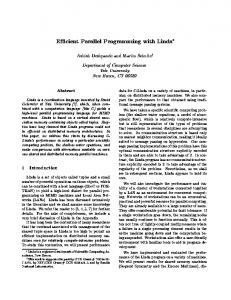
3.1 The Fujitsu AP1000 A brief description of the target architecture follows. The AP1000 is a MIMD distributed memory multiprocessor. The implementation is on a 128 cell machine. The cells are arranged in a two dimensional con guration connected in a torus network (T-net), that is, each cell is directly connected to four adjacent cells 1. Cells and host computer are connected by a separate broadcast network (B-net). The B-net is used for 1-to-N communication either by the host or a cell. The B-net provides ecient data distribution and collection between host and cells via the scatter and gather functions. A third separate network is the S-net used to communicate status and for synchronization. T-net routing is by wormhole routing so that in the absence of contention, distance is not a signi cant contribution to communication latency [29] provided message size is large. The architecture is depicted in Figure 3.1. In the normal mode of cell-to-cell message-passing, if the speci ed data is not in cache memory, the data is sent from main memory but if the data is in cache memory, it is copied to uncached memory before the send. There is a line-send mode where data in cache is sent directly from cache memory and hence, speeds up communication by a large extend by avoiding copying of data to uncached memory before the send. The line-send mode is particularly good for small data transfer since small data items are in cache memory in high possibility. There is also a message receiving feature known as buer receiving 1

With wrap around.

19

3.2. AP1000 Con guration

20 Synchronization Network (S-net)

Host Broadcast Network (B-net)

Cell

Torus Network (T-net)

Figure 3.1: AP1000 architecture. where a ring buer is created in main memory and the received message is written into this area and can be read from this area. In normal mode receiving, message data must be copied from an uncacheable message buer area before it can be read. The maximum capacity of the ring buer is 512 KB. The ring buer receiving is used with the line-send mode. Each cell has an integer unit (IU), oating-point unit (FPU), routing controller (RTC) and B-net interface (BIF) as well as a large local memory. Cache memory (CM) has a capacity of 128 KB and dynamic memory (DRAM), 16 MB.

3.2 AP1000 Con guration In the implementation, the AP1000 is con gured in one dimension (in the x direction) to match the list topology to the processor con guration. Cell programs then have a one-dimensional view. This simpli es implementation since lists are essentially onedimensional structures (though a list of lists can be viewed as having at least two dimensions).

3.3 List Data Distribution The way in which the elements of a list are distributed across the cells aects the utility of each cell, or load balance, during computations and the amount of required data motion between cells. Reducing data motion and a good load balance are important for achieving good performance. Two issues are considered when distributing the list across the cells. The rst involves treating lists of sublists. A list can contain elements which are either atomic values or lists (sublists) so that recursively, a list can consist of a hierarchy of sublists. This gives rise to two options for a list of sublists:

3.3. List Data Distribution 0

1

2

3

4

21 5

6

7

cell 0

8

9

10

11

12

13

cell 1

14

15

16

cell 2

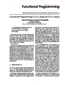
Figure 3.2: Block distribution of 17 elements over 3 cells. 0

3

6

9

cell 0

12

15

1

4

7

10

13

16

cell 1

2

5

8

11 14

cell 2

Figure 3.3: Cyclic distribution of 17 elements over 3 cells. 1. distribute the list as a attened list. For example, given a list of sublists [[1; 2; 3]; [3; 4]; [8; 90]] the list is attened as [1; 2; 3; 3; 4; 8; 90] and the 7 elements distributed across the cells. 2. distribute it using its top level structure treating each top level sublist as atomic for distribution purposes. For example, for the list [[1; 2; 3]; [3; 4]; [8; 90]], three (sublists) elements are distributed, that is, each sublist resides entirely within a cell. The second involves data allocation. Regardless of which of the above options are chosen, when the number of elements to be distributed, n , is more than the number of processors 2, p , each processor must contain more than one element. Consider the elements of a list to be indexed from 0 in its order and the cells to be indexed from 0 as well (in some order). Then, the options for allocating elements to processors include: 1. block (consecutive) allocation, aggregates data in contiguous segments of the list, one segment in each processor. An element of index i is located in processor i div (dn =p e), that is, cell 0 contains elements of indices 0,: : :,(dn =p e) ? 1, cell 1, elements of indices dn =p e,: : :,2(dn =p e) ? 1 and so on.(See Figure 3.2) 2. cyclic allocation, where data is allocated in a cyclic order with element i in processor i mod p . (See Figure 3.3) 3. block-cyclic allocation, where the list is divided into blocks distributed cyclically. If the block-size is s , an element of index i is on processor (i div s ) mod p . (See Figure 3.4) The cyclic allocation scheme could be considered a special case of this by having s as 1. These two issues are now discussed in detail. 2

cells and processors will be used interchangeably.

3.3. List Data Distribution 0

1

6

7

12

22 13

cell 0

2

3

8

9

cell 1

14

15

4

5

10

11

16

cell 2

Figure 3.4: Block-cyclic distribution of 17 elements over 3 cells using block size of 2 (s=2).

3.3.1 Treating Sublists

The BMF list operations work from the outer or top level inwards. For example, mapping a reduction to each sublist of a list, ((=); the map operation is carried out on the top level list rst mapping the reduction operation to each sublist. Then each reduction is done. Hence, distributing using the top level structure distributes the top level uniformly and seems more natural for the BMF operations. Also, distributing the list of sublists using the top level structure simpli es computations or operations on the list. For example, suppose a list of sublists is distributed across the processors as a attened list and each sublist is distributed across several processors (possibly dierent number of), then performing operations between any two sublists of the list (say during a reduction with operations like zip (1( =) or matrix multiplication (where each matrix is represented as a list of sublists in row or column major order)) may involve more complex communication. However, the choice of distributing using the top level structure causes parallelism to be at the top level only and not at the sublist levels. Exploitation of parallelism at the sublist levels means more parallelism but there is more communication [30]. Parallelism at the sublist level is more important when the number of processors available is large (at least a factor of two) compared to the number of elements at the top level, otherwise not much performance increase will be obtained. For example, in Blelloch's scan-vector model, a list of sublists is distributed as a attened list on the CM-2 with 8 to 64 K processors. In this implementation on a machine with 128 cells, it would be more suitable to distribute the list using the top level structure since the number of elements at the top level would be expected to often exceed the number of cells. Distributing using the top level structure may also cause poor load balance for irregular sublists, that is, when the length of the sublists vary. However, if the length of the sublists vary randomly, and if there are several sublists on each processor, the probability of good load balance is high. x3.3.2 discusses the data allocation when n p . Given the above, this implementation distributes the list using its top level structure.

3.3.2 Data Allocation

All data motion or communication involved in a program formulated with these functions are embedded within these functions. Hence, the data must be allocated so as to support ecient implementations of the BMF functions, namely reducing the data motion required in computing these functions. The allocation must also as far as possible provide good load balance for programs. Block (consecutive) allocation is generally preferred for computations where nearest neighbour references dominate since this reduces communication. Operations like pre x, reduce, recur pre x and recur reduce are by de nition operations that use nearest neigh-

3.3. List Data Distribution

23

bour references, that is, the associative binary operator is applied between adjacent (in the order of the list) elements of the list. Hence, consecutive allocation of the list elements would be most suitable for these operations with respect to communication. However, in some programs, consecutive allocation may lead to poor load balance due to computations being non-uniform across the index space. For example, in doing a crude numerical integration with several data points per processor, if the function to be evaluated at each point is given by a series, some processors may have less work. Another example is triangular matrix product where (the matrix is distributed over the cells as a list of rows) computations will be more intensive on cells with more (non-zero) data (shown in Chapter 5). Cyclic allocation gives better load balance for some computations like the one mentioned above. In other computations a cyclic allocation can give better performance by reducing communication needs. For the operation of concatenating two lists, cyclic allocation causes the costs to depend on the number of processors rather than on the length of the concatenated list. For example, to do a concatenation with cyclically distributed lists, the second list is rotated till its rst element is on the cell with the last element of the rst list. However, operations like reduce with concatenate or pre x with concatenate will be easier to implement with consecutive allocation of the sublists since concatenate is associative but not commutative. A best case example is that sublists of the same length can be concatenated with no communication if the sublists are consecutively allocated. Only an internal concatenation operation (or type coercion) is required within each cell. The result list is distributed. So far, the only requirements for the operators used in the higher order functions are that they are associative. Now, if the operator(s) used in a particular reduction (or recurreduce) is commutative like addition, then the order of the elements of the argument list does not matter. Regardless of the allocation of the list elements, computing using the same (optimal) tree-structured algorithm for reductions (with rst stage local sequential reductions on each processor and second stage global tree reduction across the processors) gives the same result. However, for operations like pre x and recur-pre x, even if the particular operator(s) used are commutative like addition, computing using the same tree-structured algorithm (described in x3.5.2) but with dierent allocation schemes can give dierent results. The algorithm required to compute pre x operations if the data is allocated cyclically or block-cyclically is dierent from that used for consecutive allocation. The algorithm for parallel-pre x based on consecutive allocation would require less communication than the algorithm based on cyclic (or block-cyclic) allocation which computes the same result because of nearest-neighbour references. For computations where consecutive allocation gives poor load balance, a block-cyclic allocation scheme may be used to give better load balance without signi cantly increasing data motion for the pre x and reduction (with associative but non-commutative operator) operations. However, deciding on a suitable block size is a problem. As block-size varies, there is a tradeo between data motion and load balance. In summary, the choice of the data allocation can aect the algorithms for the BMF operations, in particular the more important (more commonly used) reduce (with associative operator) and pre x operations. A consecutive allocation of the data elements

3.4. Implementation on the AP1000

24

minimises data motion but can give rise to poor load balance. Cyclic (or block-cyclic) allocation which can give better load balance can be used for programs where operators used, in say reductions (reduce or recur reduce), are commutative without compromising on the performance of reduction operators but with the limitation that pre x operators (if used in the program on a distributed list) are computed with an algorithm which has more communication than the algorithm for pre x with consecutive allocation.

3.4 Implementation on the AP1000 The remainder of this chapter describes the implementation using the block allocation scheme. In Chapter 5, implementation with the block-cyclic scheme is described and its performance compared with that of the block scheme. The data structure and algorithms used for the implementations are given in the following sections. Using the block-cyclic scheme, the algorithms will be dierent from that using the block scheme (the block scheme implementations are less complex). The data structures, function prototypes and a small communication library described here are reused for the block-cyclic scheme.

3.4.1 List Data Structure

Each cell contains a part of the distributed list. One view of the block allocation using BMF is to treat each block in each cell as a sub-list (segment) and the entire list as the concatenation of all these segments as shown below: [0; 1; 2] ++ [3; 4; 5] ++ [6; 7; 8] cell0 cell1 cell2 that is, when the list is distributed, there is a `lifting' into a list of sublists given by a mapping dis : [] ! [[]] where for example, dis [0; : : : ; 8] = [[0; 1; 2]; [3; 4; 5]; [6; 7; 8]], that is, ++= dis = id . Data structure alternatives considered for the list segment (within each cell) are: 1. linked-list. A list segment is implemented by a linked-list. If it is a list of sublists, it is represented by a linked-list with each node pointing to a linked-list. 2. at array. A list segment is represented using C arrays. If it is a list of sublists, arrays are used to represent the at list and hierarchical information (provided to determine the sublists lengths). For example to represent the list [[[a ; b ]; [c ; d ]]; [[e ]; [f ]]], we use three arrays: flat list = hierarchy1 = hierarchy2 =

[a ; b ; c ; d ; e ; f ] [2; 2; 1; 1] [2; 2]


25

3. array. A list segment is represented using a (one-dimensional) C array but if it is a list of sublists, it is represented eectively by an array of pointers to arrays. Alternative (1) provides exibility in manipulating the list, that is, deleting from and adding an element to any position in the list-which may be useful for shortening and lengthening the list dynamically in say the lter operation. However, it takes up more memory per element since a full structure is required to store the element and a pointer to the next node. Also, in transferring even a list of atomic values, each element needs to be packed into an array before it can be sent to another cell. Accessing elements of the list is also slower than array element access. This is because of the extra indirection of fetching the address of the next node. Alternative (2) involves manipulating the hierarchical information each time an operation is done on the list. Extracting a sublist with its own hierarchical information is cumbersome. Also, expanding the list, say in a map operation that converts each element of the list into a sublist is cumbersome and involves a great deal of array copying in creating the new at array and the hierarchical information. Alternative (3) is chosen since array element access is relatively fast. Also, transfer of a list of atomic values can be done without packing. Transfer of a list of sublists can be done recursively. Also, no hierarchical information needs to be manipulated.

3.4.2 Types and Function Prototypes

This section discusses the types supported in the implementation. Lists and the BMF functions are polymorphic, that is, lists can be of any type and the operations will have to deal with lists of any type. Polymorphism in the extent of pure functional programming languages like Miranda would be ideal but this implementation in C does not go that far. Instead only a subset of types is implemented. As mentioned, every element of the list is of the same type and that a list may be a list of lists. The main types implemented can be given as follows. Let T be the set of types implemented. Then: 1. atomic types (C base types): char, integer, float 2. pairs: (, ) 2 T , where , 2 T .

(single-precision)

2 T.

3. lists: [] 2 T , where 2 T 4. Only the above are in T . A ground type (called GENTYPE) which is a union structure of a int and a float is used to implement the above types. This allows storage of floats or ints or a memory address in a memory location.

Pairs and Lists Pairs and lists are C structs:

struct

pair

f

< type info for c 1 and c 2 >


g

GENTYPE GENTYPE

26

c1; c2;

and (logically, a list is represented by its tag and its data).

struct

f

list /*tag*/ element-type; length; distributed;

int int int

g

/* list data */ data;

GENTYPE*

/* array of elements */

is an array of elements of type element-type of length length (length of list segment) and distributed determines if the list is a segment of the globally distributed list or an element of a list which is a sub-list (entirely local within a cell). The size of ints is 4 bytes on the AP1000. For list elements of size less than or equal to 4 bytes (the atomic types), the int element values are stored within the data array. For list elements of size more than 4 bytes, each element of the data array is a pointer to a C struct containing the list element value. For lists of sublists, each element of the data array is a pointer to a struct list structure. data

Functions Function parameters to higher-order operations use a structure, fn info, encapsulating a pointer to the function and its return type (the return type eld is necessary for type changing operations such as map.). Function parameters are either unary or binary functions and have the following C prototypes: void f(GENTYPE,GENTYPE*); void f(GENTYPE,GENTYPE,GENTYPE*);

For the BMF functions, the result is returned in the same way as above, in the parameter GENTYPE*. An example function prototype is as follows: void recur_reduce(fn_info /*bop1*/,fn_info GENTYPE /*list1*/,GENTYPE /*list2*/, GENTYPE /*seed*/,GENTYPE* /* result */)

3.4.3 Communication Library

/*bop2*/,

A small library of communication functions was implemented on top of the AP1000 library functions [31] comprising the following:

3.5. Implementing the Functions Using Block Distribution c_recv_elmt c_send_elmt c_brd_elmt c_broad_elmt

, , , ,

using using using using

27

l_arecv l_asend x_brd c_broad

The functions make use of the element-type eld in the list struct to determine what is sent (broadcasted) or received between cells. Data of a list of atomic elements are sent in one message. Recursive structures such as lists of lists are transferred between cells recursively, that is, they are sent and received recursively according to their structure so that any of the above functions may call itself recursively. For example, to send a list of sublists, each sublist is sent and received separately. To determine the size and type of received messages, sending of message tags precedes the sending of structured types such as lists or pairs (message tags are not used for transferring atomic elements). The use of tags incurs a communication overhead but this overhead would be less signi cant if the data transferred is large, eg. long sublists. An alternative for list of sublists transfer is to pack data into a at array before sending and unpacking it on receiving. For example, in sending a list of sublists, do 1. pack [[: : :]; : : : ; [: : :]] = [: : :] 2. transfer (packed list), [: : :], and tag (including hierarchical information). 3. unpack [: : :] = [[: : :]; : : : ; [: : :]] This method has the overhead of packing and unpacking particularly for long sublists and for deeply nested lists and hence, is not used.

3.5 Implementing the Functions Using Block Distribution 3.5.1 Overview

In the experiments that follow in the next chapter, the data for the distributed list is initially stored on the cells rather than distributed from the host. This means that the amount of data can be up to the sum total of the cell memories rather than be limited by the host memory. The nal result of computations reside on the cells and can be collected by the host (if not too large). Single value results (say of reductions) end up in cell 0. The BMF routines are called from the cells, that is, programs (composition of functions) are executed in an SPMD (or SFMD) way. The distributed eld of the list structure, if the list is distributed, indicates the number of cells over which the list is distributed to avoid computing over redundant cells with no data, particularly, when the list is distributed over fewer than the number of cells the AP1000 is con gured with.

3.5. Implementing the Functions Using Block Distribution

28

Redistribution For operations which take two list arguments such as zip, recur reduce and recur pre x, the algorithms are simpler when both their list arguments are distributed in exactly the same way, that is, a standard way for the distribution of lists is maintained. This is: elements of indices 0; : : : ; (dn =p e)?1 reside in cell 0, elements of indices dn =p e; : : : ; 2dn =p e?1 reside in cell 1 and so on (as seen earlier). This is a precondition for all functions taking lists as arguments; that the lists must be distributed in the standard way. This also implies a postcondition that result lists should be distributed in this way as well 3. Several operations return results which have size of data or length dierent from their distributed list(s) argument(s). These are lter, cross product and recur pre x. For these operations, the algorithm include the overhead of maintaining the standard distribution of the list. This amounts to redistributing list elements among cells in some cases.

3.5.2 Algorithms

In this section, the algorithms for the functions map, reduce 4, pre x 5 recur reduce, recur pre x, inits, tails, cross product, zip and lter using block distribution of list arguments are given. Although it is shown in the previous chapter that many of the operations can be computed as a composition of a map and a reduction, direct implementation as a single operation is more ecient (the next chapter shows some overheads of computing compositions). Serial Versions Most of the serial versions of the operations can be computed in O (n ) serial time in one or two passes (using C for loops) through the list (loop fusion could be used to compute using one pass through the elements) except for inits and tails which can be computed in O (n 2) serial time and cross product in O (mn ) time (with an argument of length m and an argument of length n ). The serial versions are used for some performance comparisons presented in the next chapter. The rest of this chapter focusses on the parallel versions of these operations. The parallel operations involve serial computations of the operations as well. Parallel Versions (using block distribution) Whenever possible, the idea of implementation equations, which uses the BMF itself to describe algorithms, in [32, 30], is used here to express the algorithms in a concise and high-level way. These equations also help in estimating the parallel time complexity of the computations. As in [32], to simplify descriptions, the following are assumed: A special case is where the result of a reduction is a list. In the implementation of reduce given later, the result list will reside entirely in one cell. An additional (costly) step is required to distribute the list across the cells if required. Some discussion of this is included in Chapters 6 and 7. 4 Not directed reductions which are inherently linear but reduction with an associative binary operator. 5 Not accumulations which are inherently linear but pre x with an associative binary operator. 3


29

1. the number of elements of the list (at the top level), n p , the number of cells. When n > p the algorithm has a sequential and a parallel part since there will be more than one element per cell. 2. p divides n. 3. constant cost of binary operations (() and unary operations that are parameters to the functions. This would not be true for operations like concatenation (++) whose cost depends on the size of its arguments. 4. cost of transferring an element between cells is constant unless otherwise stated. This would not be true for say, ++= since larger lists are communicated between cells as each step progresses. Detailed algorithms in the imperative style are given in Appendix C but two examples are presented here to show the correspondence of implementation equations with actual imperative code. The implementation equations view a distributed list as a list of sublists, each sublist segment in a cell, as described in x3.4.1 earlier. Overbars are used to indicate the sequential part of an operation, subscripts indicate the number of elements to which an operation is being applied (in parallel or sequentially). Also, two rules that (the rst of which resembles the map composition property) apply to sequential version of operations are: f m g m = (f g )m (f m )r = f mr

The right hand side of the rst equation indicates the fusion of the two loops of f and g .

map. The map function requires no communication. Map has the following implementation equation:

f n = (f n =p )p (Note that the implementation equations have an apparent type mismatch between the left and right hand sides. This is resolved by the implicit application of the earlier de ned dis function in x3.4.1 on the list before the right hand side is applied.) The above equation means that a map operation over a list of length n is implemented by executing a serial map on arguments of length n =p in parallel (as suggested by the ) on p cells. The imperative algorithm is as below:

map(f)

/* do serial map: f n =p */ for i := 1 to (length of arg list) do result list[i] := f(arg list[i])

endfor endmap

3.5. Implementing the Functions Using Block Distribution cell

0

1

2

3

4

5

6

30 7

time-steps

Figure 3.5: Skewed binary tree reduction.

reduce. A reduction is computed on a distributed list as follows: 1. do sequential reduction on local block within each cell 2. do global parallel reduction across the cells This is represented by the implementation equation:

(=n = (=p ((=n =p )p The right hand side of this equation reads as èxecute p sequential reductions over arguments of length n =p in parallel on p cells, and then, do a parallel reduction across p cells'. The parallel reduction ((=p part) is done by means of a binary tree-structured communication pattern, skewing to the left as shown in Figure 3.5, so that the estimated complexity for the whole reduction operation is log p + n =p as inferred from the implementation equation with logarithmic steps for the parallel part and n =p cost for the sequential part. The nal result of a parallel reduction resides in cell 0 only. A more detailed algorithm is as follows which computes (= on some argument list:

reduce(() if (length of arg list) > 0 then /* do serial reduce: (=n =p */

result := arg list[1] for i := 2 to (length of arg list) do result := result ( arg list[i]

endfor else


31

result := id( return /* done */

endif

if arg list is part of a distributed list then /* do parallel reduce: (=p */

curr oset := 1 cells := number of cells over which whole argument list is distributed

do

prev oset := curr oset curr oset := curr oset * 2 if (this cell id mod curr oset) = 0 then if (this cell id+prev oset) < cells then recv elmt := receive from cell(this cell id+prev oset) result := result ( recv elmt

endif else if (this cell id mod prev oset) = 0 then if this cell id prev oset then send to cell(this cell id-prev oset,result) endif endif while curr oset cells endif endreduce

pre x. A pre x computation is carried out on a distributed list as follows: 1. do a sequential pre x on the local block within each cell 2. do a global parallel pre x operation with the last value of the sequential pre x result 3. do right shift one step on the result of the global pre x 4. add the value from the shift to each element of the result of the sequential pre x The following example computing: + == [0; 1; 2; 3; 4; 5; 6; 7; 8; 9; 10; 11] illustrates the algorithm. The initial list is distributed as follows. C0 C1 C2 C3 0 3 6 9 1 4 7 10 2 5 8 11 After the sequential pre x on each cell:


32

C0 C1 C2 C3 0 3 6 9 1 7 13 19 3 12 21 30 A parallel pre x is then computed using the last value in each block followed by a shift right one step: C0 C1 C2 C3 0 3 6 9 1 7 13 19 3 12 21 30 0 3 15 36 and the results of the shift are then added to all the values (above them in the diagram) within each block: C0 C1 C2 C3 0 6 21 45 1 10 28 55 3 15 36 66 The above algorithm can be expressed as:

(== = ((x ()n =p )p shift ( ==p ((==n =p )p where x is a result of the shift right operation and shift (==p is applied to the last element of the local segment of each cell. (Although the shift operation could be done rst and a parallel pre x over n ? 1 number of cells, when the number of cells is say 128, there is little dierence in eciency.) Two alternatives are considered for computing the parallel pre x operation, that is, the (==p part. two phase algorithm. This algorithm does an up-sweep and a down-sweep in a treestructured communication pattern. This algorithm is presented in detail in [30]. In the rst phase or the up-sweep, a reduction is computed across the cells. In the second phase or the down-sweep, partial results are passed back to other cells to be computed with the values in those cells. A small example is shown in Figure 3.6. Here, the arrows between columns represent the data ow between cells. More generally, the operations carried out in the cells at each step in the up-sweep is given in Figure 3.7(i) and for the down-sweep in Figure 3.7(ii).

single phase. This algorithm does the parallel-pre x computation in a single phase

in logarithmic steps. The right skewed tree-communication pattern is as shown in Figure 3.8. In the rst step, each cell sends to its right neighbour and receives from its left neighbour. In the next step, each cell sends to a cell two cells away (on the right) and receives from a cell two cells away (on the left). In the third step (not seen in the example of Figure 3.8), each cell sends to a cell four cells away and receives from a cell four cells away and so on - doubling distances each time and always sending and receiving only when the cell that distance away exists.

3.5. Implementing the Functions Using Block Distribution C0

C1

C2

C3

[3]

[12]

[21]

[30]

3

12

21

33

30

[3,12]

[21,30] 15

51 [15,21,30]

[3,12]

[36,30] 15

[3]

[15]

[36]

[66]

Figure 3.6: Data Flow for 2-phase parallel pre x

@

R

@

l1 @

R

R

R @

?

? l? ? R ! [(l + fR)] ++ (tR) [(fR + SR )] + + (rR ) ? fR ? ?l

l1 @

R ?l2 @ [l1 ] + +R @ l1 ( l2@

R ?l2 @ [l1 ] + +R l1 ( l2

?? ?

?

?

(i)

?

(ii)

R is a list, l1 and l2 are list elements and ! means `change to'. f ,s ,r and t are de ned by: f [a1; a2 ; : : : ; an ] = a1 ,and , s [a1; a2 ; : : : ; an ] = a2 r [a1; a2 ; : : : ; an ] = [a3; : : : ; an ] ,and , t [a1 ; a2; : : : ; an ] = [a2; : : : ; an ]

Figure 3.7: Operations performed at each cell. C0

C1

[3]

[12] 3

[3]

[15] 3

[3]

C2

C3

[21] [30] 12 21 [33]

[51]

15 [15]

[36]

[66]

Figure 3.8: Single phase pre x example


34

Several points of comparison between these algorithms are: 1. The single phase algorithm takes log p steps rather than 2log p steps. Although there is more communication in each step of the single phase algorithm, there may not be serious contention as all messages are to dierent destinations and travel in the same direction and for the same distance, particularly if the messages are small. Otherwise, contention may slow down each step signi cantly. 2. In the single phase algorithm, most of the cells are kept busier (either doing a computation or at least doing a send) than when the two phase algorithm is used this would mean better utility of the cells. 3. The two phase algorithm requires storing and manipulating small lists of partial results in each cell at each step during its phases. The single phase algorithm only stores one value in each cell, the current computed value at each step. The above seems to be in favour of the single-phase algorithm in terms of eciency unless the contention cost is high. In terms of theoretical complexity, from the implementation equation for pre x, it is n =p + 1 + log p + n =p for the single phase algorithm and n =p + 1 + 2log p + n =p for the double phase algorithm (cost of 1 for the shift). Quantitative comparisons are carried out in the next chapter.

zip. Zip is computed in a similar way as map (without need for communication) and its implementation can be given by: ( 1( )n = (( 1( )n =p )p When its two list arguments have dierent lengths, the excess data of the longer list can either be dropped or concatenated to the result of zipping both the lists up to the length of the shorter list. In this implementation of zip, the èxcess' data is dropped.

lter. When the lter operation is computed on a distributed list, the operation may

shorten the list, load balancing needs to be done (also to avoid `gaps' where there are cells with no remaining elements but its neighbours have some remaining elements). After the load balance, if the list has been shortened by the lter operation, the elements of the new list gather on the lower numbered cells. A pre x operation is needed to index the elements of the new list and to determine the length of the new list. The indices are required to do a redistribution of the remaining elements - eectively a load balancing operation. The computation to index the elements of the new list can be expressed as follows: Let Ki be the constant function given by Ki x = i , for any x . Indices are computed by: + == (if p then K1 else K0), for predicate p used as parameter to lter. Each processor ends up with a block of the new list (of remaining elements satisfying p ). The block is returned by this function in the cells. Computation of lter on a distributed list is as follows: 1. compute + == (p ! K1 ; K0)


35

2. do redistribution (load balancing) operation (a) broadcast the length of the new list to all cells from the last cell (b) compute the number of elements of the new list each cell should have (c) determine the cell destination and local index for each remaining element (element satisfying p ) in each cell (d) pack elements with the same destination cell together and send the elements to their destination cells (e) receive elements from other cells and store them using the local index The rst step can be expressed using the implementation equation: ((x +)n =p )p shift + ==p ((+ == f )n =p )p where f = (p ! K1; K0). Broadcasting of the length is done using x brd and cell-to-cell element transfers with c send elmt and c recv elmt. The time complexity of lter is at least that of the pre x plus a map operation. The next chapter discusses the costs of the load balancing operations in more detail.

inits. Inits can be computed as follows: 1. do a serial inits operation with the block in each cell 2. do parallel inits The parallel inits can be computed either by circulating values using a Hamiltonian cycle, each cell accumulating the parts of the initial list to form its segments or by a communication pattern just like the pre x communication pattern - a right skewed tree pattern. The algorithm using the Hamiltonian cycle computing inits[a0 ; a1; : : : ; a7] is illustrated below. C0 C1 C2 C3 a0 a2 a4 a6 a1 a3 a5 a7 After the serial inits within each block: C0 C1 C2 C3 a0 a2 a4 a6 a0 a1 a2a3 a4 a5 a6 a7 Each cell (except the last) then passes its longest sublist to its right neighbour which prepends it to each of its elements: C0 C1 C2 C3 a0 a0a1 a2 a2 a3a4 a4a5 a6 a0a1 a0 a1a2 a3 a2a3 a4a5 a4a5 a6a7 For each cell (except the rst in this step), the same sublist that was received from the left neighbour is then passed on to the right neighbour, that is, the initial longest


36

sublist in each cell have circulated two steps from their originating cell. Then, each cell on receiving the sublist prepends it to its current partial results: C0 C1 C2 C3 a0 a0a1 a2 a0 a1a2 a3a4 a2a3 a4a5 a6 a0a1 a0 a1a2 a3 a0a1 a2a3 a4a5 a2a3 a4a5 a6a7 One more step, C2 passing a0 a1 to C3 followed by prepending of this to elements in C3 completes the computation. The implementation equation is: initsn = ((prepend n =p passright )p )p (initsn =p )p

For the parallel operation, there are p prepend passright operations. A sublist of length n =p is transferred in each passright and each prepend (n =p of them) is with a sublist of length n =p so that each prepend passright operation above takes n =p + (n =p )(n =p ). So, in total, a cost of O (n 2=p ) for parallel operations. The cost of serial inits is O ((n =p )2). Hence, the estimated overall cost is O (n 2=p ). Computing the parallel inits part using a pre x communication pattern is motivated by the equality inits = ++ == [] The implementation equation is: initsn = ((x ++)n =p )p shift ++ ==p ((++ == [])n =p )p

where (x ++) is prepending with x . In computing inits as a single operation, the sequential part of the pre x and the [] operation is done at the same time (equivalent to fusing the two loops). Cost of ++==p has been estimated in [30] to be O (n 2=p ) with a two phase pre x algorithm so that that becomes the estimated overall cost. The cost of ++==p was estimated taking into account increasing message sizes (cost of message transfer being proportional to message size). However, with suciently small messages (with small grain size), the cost may be over-estimating (the eect of the increasing message size is not felt). Quantitative comparisons are made in the next chapter between the cost of inits using single phase pre x and the cost of inits using the Hamiltonian path.

tails. Tails is computed in a similar way as inits with a serial and then a parallel step

except that the parallel part circulates the elements in the opposite direction to that of inits. This is because from its de nition, the longer sublists are on the left part of the result list (as oppose to inits where, in the result, longer sublists are on the right). Using the Hamiltonian path, the algorithm is similar except that the sublists are passed left. In the pre x-style, the algorithm uses a tree-communication pattern like that of pre x but which skews left instead of right and append instead of prepend .

recur reduce. The computation of recur reduce is similar to that of reduce. The im-

plementation of the algorithm is suggested by the following de nition of recur-reduce [28]: ( #x (= #y ) = 0 x ) =e ( y = ee ;) A ( A; ifif # x (= #y ) 6= 0 1

2

3.5. Implementing the Functions Using Block Distribution C0

C1

C2

C3

s1

s2

s3

s4

s12

37

s34

A

Figure 3.9: An example recur-reduce operation. s 1 = (a1 ; b1), s 2 = (a2 ; b2), s 3 = (a3 ; b3) and s 4 = (a4 ; b4). s 12 = (a1 ) a2 ; b1 ) a2 ( b2), s 34 = (a3 ) a4; b3 ) a4 ( b4). A = (a1 ) : : : ) a4 ,b1 ) a2 ) a3 ) a4 ( : : : ( b3 ) a4 ( b4). where A a-b (a ; b ) + (c ; d ) 1(a ; b ) = a

= = = and

+=(x 1- y );

(a ; b ); (a ) c ; b ) c ( d ); 2 (a ; b ) = b

Figure 3.9 shows an example of the formation of A as de ned above. Local block recur-reduction within each cell is done before the global recur-reduction operation across the cells. The communication pattern involved in the global recurreduce operation across the cells is binary-tree structured, similar to that for reduce; clearly since the above de nition shows that a reduction is involved. From the de nition above, the reduce and zip operators could be used to compute this function but a direct implementation (overlapping code) is more ecient. The implementation equation to build A in the de nition above is:

+=p (+=n =p )p (( 1- )n =p )p =

8 >
: and combining loops +=p ((+= ( 1- ))n =p )p

9 > = > ;

with a cost of O (log p + n =p ) (not simpli ed fully to show the breakdown) as worked out in [30]. In the above equation, the loop for the reduction and zip are fused in the implementation. The algorithm is explained in detail in [30].

recur pre x. The recur pre x operation is similar to that of the pre x operation. The implementation algorithm is suggested by the following de nition of recur pre x: x ) ==e ( y =

(

[e ]; if #x (= #y ) = 0 [e ] ++ (e *) (+ == (x 1- y )); if #x (= #y ) 6= 0


38

where

a - b = (a ; b ); (a ; b ) + (c ; d ) = (a ) c ; b ) c ( d ); e * (a ; b ) = e ) a ( b From above, the pre x, zip and map operations could be employed to compute this function. However, it is computed directly since this is more ecient. The operation takes the same arguments as recur reduce. The algorithm given here computes a sequential recur-pre x on the local block and then does a global parallel recur-pre x operation across the cells in a way similar to the pre x algorithm. However, the nal results are obtained after a map operation (e *), and after the seed element, e , is added to the list as the above de nition shows. Its implementation equation is: )==e( = shiftrighte ((e *)n =p )p (((x ; y )+)n =p )p shift + ==p ((+ == ( 1- ))n =p )p

with a cost of O (log p + n =p ) (not simpli ed fully to show the breakdown) as worked out in [30]. The algorithm is also explained in detail in [30]. A redistribution of elements after the last shiftrighte operation is needed in some situations as described below. Implementation wise, the shiftrighte involves introducing e at the head of the intermediate result list and each cell (except the last) sending an element to its right neighbour eecting the shift. For example, suppose we have the distribution (and there are only 3 cells): [r0 ; r1 ; r2 ] ++ [r3; r4 ; r5 ] ++ [r6 ; r7] cell0 cell1 cell2 just before the shiftrighte is to be performed. Then when e is introduced in cell 0, r2 goes to cell 1 and r5 to cell 2 so that we have, [e ; r0 ; r1 ] ++ [r2; r3 ; r4 ] ++ [r5 ; r6 ; r7] cell0 cell1 cell2 In this case, the cost expression shown earlier applies. However, a deviation arises if the last cell is already full, Suppose now cell 2 already has 3 elements just before the shiftrighte operation. Then, the last cell will end up with 4 elements after this shiftrighte operation. Then, to obtain the nal result list in the standard distribution, a redistribution is carried out from [e ; r0 ; r1] ++ [r2 ; r3 ; r4 ] ++ [r5; r6 ; r7 ; r8 ] cell0 cell1 cell2 to [e ; r0 ; r1; r2 ] ++ [r3 ; r4 ; r5 ; r6] ++ [r7 ; r8 ] cell0 cell1 cell2 The cost of this additional redistribution depends on the number of elements that needs to be redistributed. The redistribution is carried out in similar way as in lter.


39

cross product. Computation of the cross product operation requires each element of

the rst argument list to interact with every element of the second argument list. With both lists initially distributed across the cells, the rst argument list needs to be brought to each cell containing the second argument list. The result of the cross product is distributed across the cells. Two alternative algorithms are considered for cross product:

Using the Hamiltonian path. In this algorithm, the rst argument list is circulated

round to the cells containing the second argument list where the binary operations are then applied between the elements of the circulated list and the elements of the segment of the second list within the cell. The algorithm is given by: 1. Each cell computes a local cross product with the segments of both argument lists it has (if a cell has a segment of only one of the argument lists, it waits) 2. Each cell then passes its segment of the rst argument list (if it has received one or initially, if it contains one) to its right neighbour (wrap around if last cell) and receives a segment (of the rst argument list) from its left neighbour (wrap around if rst cell). 3. In each cell, local cross product is then computed between the received segment and its local segment of the second argument list (if the cell contains one). 4. Steps 2 and 3 are then repeated till the rst argument list has been circulated to all cells containing the second argument list.

The results of the partial cross products computed as the argument segments are circulated must be stored in the nal result segment in the right order since the algorithm does not compute them in the right order. Using the broadcast facilities of the AP1000. Each cell containing a segment of the rst argument list broadcasts its segment to all cells containing a segment of the second argument list. This can be done either with the T-net or B-net broadcasts. The algorithm is as follows: 1. Each cell broadcasts its segment of the rst argument list (if the cell has one) to all other cells. 2. For each segment received, a local cross product is then computed with the received segment and with the local segment of the second argument list (if it has one). Again, if the segments are broadcasted in some order, say starting with cell 0 , then cell 1 and so on, the results must be stored in the right order in the nal result segment within each cell (containing a segment of the second argument list). In both cases, a nal redistribution operation is required to ensure that the nal result list is distributed in the standard way. An example which illustrates this (using the Hamiltonian path) is shown in Figure 3.10. The redistribution phase is carried out in the same way as for lter. The above alternatives are compared on their performances in the next chapter.

3.6. Auxiliary Operations

40

C0

C1

C2

arg1

5

5

5

arg2

3

3

3

C3

5

after 4 steps of circulating arg1

result

60

60

60

redistribution

final result

45

45

45

45

(standard distribution)

Figure 3.10: A cross product operation with rst argument of length 20 and the second argument of length 9 both initially distributed across the cells (in the standard way mentioned earlier). In performing the operations, the result list needs to be redistributed. This ensures that lists of exactly the same length (180 in the above case) are distributed in exactly the same way. The numbers in the rectangles represent the number of elements in a block. Arrows across columns represent data ow between cells.

3.6 Auxiliary Operations Some other operations needed but are not part of the library of functions includes the replicate function, @, which takes two arguments, n and a , and creates a (length n ) list of replicates of a , n @a = [a ; : : : ; a ] n @x could be computed by ([] x ) 2 [: : :] where [: : :] can be any list of length n and is the `left' operator given by a b = a . However, implementation as a special primitive is more ecient. List generation functions are also implemented which generates lists of given length and type, in particular lists of ints and floats (and lists of lists) used in example computations. Other housekeeping operations such as assemble and distribute, dis , would need to be implemented to assemble results (lists) back from the cells to the host and to distribute argument lists to the cells from the host respectively if the original data are stored in the host. List constructor operations like [] and ++ required in computations frequently are also implemented.

3.7 Implementing Sectioning As mentioned earlier, some operations may be sectioned. Immediate examples of these are (= or just (x (). Implementing this in C was done by using global variables and declaring a new C procedure to represent the new function formed. For example, (x ()

3.7. Implementing Sectioning

41

is implemented by storing x as a global variable and de ning a new procedure which computes (x () using the global variable and calling the procedure that computes (. This would be sucient for sequential applications but for operations such as (x (), where for the map to compute in parallel, the data x needs to be broadcasted to all cells at the start of the computation. If x is itself a list which is distributed across the cells initially, this may involve all cells broadcasting its segment to all other cells or collecting x in one cell and broadcasting it to all other cells. Alternatively, x can be loaded onto the cells from the host before computations (if the data resides on the host initially). In any case, the implementation requires an implicit broadcast of x to the cells. This leads to a speci c version of map, (f x ), for some function f and argument x where f x is a function.

Chapter 4 Performance Evaluation In this chapter, the performance of the implemented library of communication functions described in the previous chapter is evaluated. As indicated in the previous chapter, parallel versions of the operations would usually include serial computations so that serial performances aect performance of parallel computations. The performance evaluation is done in two parts: 1. Evaluation of serial versions of the operations to investigate overheads (identifying sources of ineciencies) in serial computations, when computing using the list CDT. This is via comparing the performance of several sequential computations formulated using the library functions with the performance of their equivalent (in the sense of computing the same function) program hand-coded in C in the imperative style. The examples used are fairly simple algorithmically and thus, the hand-coded C code for these examples are straightforward. Also, in the examples, the performance improvement of using a single operation to compute a composition of two functions rather than using the component functions is measured - that is, measuring eciency gains of using one function, instead of two, which allows overlapping of computations. The measurements were taken on a machine with a SPARC-2 processor 1. 2. Evaluation of parallel versions of the operations. The actual parallel performance of the individual functions are compared with that of the theoretical complexity estimations given in the previous chapter. Also, the parallel eciencies of function compositions are compared with that of more direct implementations. Costly operations and barrier synchronization are brie y discussed. The performance of parallel versions of the serial program examples used in part 1 above and several other parallel examples are evaluated.

4.1 Evaluation of Serial Computations For each comparison, the hand-coded C code and the equivalent computation using the list CDT are given. 1

which is roughly 1.6 times faster than the SPARC-1 of the AP1000 cells

42

4.1. Evaluation of Serial Computations

43

Inner Product Cmputations

3.5

hand-coded C 3 + += ( 1 ) 2

3 2.5 execution 2 time(s) 1.5

2

2

1

2

0.5

2 2 + 2+ 3 +3 03 0

+ 3

+ 3

100 200 300 400 500 6003 700 vector length(10 )

+ 3 800 900 1000

Figure 4.1: Comparing inner-product computations using normal hand-coded C, as a function composition and as a single serial operation.

4.1.1 Inner Product

The inner-product of two vectors v and w represented as arrays of floats (single-precision) can be computed by: ip = 0.0; for(i=0 ; i < n; i++) f ip = ip + v[i] * w[i];

g

The performance of this is compared with that of the following computation of the innerproduct expressed as a composition of a reduce and a zip: Innerproduct (v ; w ) = +=(v 1 w )

and with an operation which computes the inner-product in a single operation using similar code as that shown above for the hand-coded C version. Denote this operation by (call it inner product).

Performance. The graph shown in Figure 4.1 shows the execution time. Not surpris-

ingly, the performance of the hand-coded C version and that of the new inner-product operation are almost same since they both use similar code. One dierence between inner product, , and the hand-coded C version is that the data in inner product has to be accessed from a list struct. So, the above results also shows that additional dereferencing required to access the data array from the list structure does not appear to be signi cant. Both performances were at about 9 MFLOPS with vector lengths of 1000 and


44

5000, 6 MFLOPS for vector length of 10000 and about 5 MFLOPS for longer vectors. The drop in performance would be due to cache eects as longer vectors will not t into the cache. The performance of the composition was consistently at about 0.6 MFLOPS, about a factor of 9 slower. Other results show that two-thirds of the total computation time was spent in the zip operation and the rest of the time in the reduction operation. Sources of ineciencies include construction of the intermediate result returned by the zip operation. This involves memory allocation and additional memory references during the one pass over the two vectors in the zip and the single pass through the intermediate result of the zip in the reduction. Also, each addition operation in the reduction and each multiplication operation in the zip is done via a procedure call causing overheads. This separation of addition and multiplication prevents taking advantage of the capability of most modern high-performance

oating point processors of performing concurrent add and multiply. Also, intermediate results of multiplications could not remain in registers to be used for additions as is possible with computing the multiplication and addition together.

4.1.2 Approximating Integrals

The computation here is to compute approximations to the de nite integral using the midpoint rule, that is, the sum Qf : Qf = I

Rs

r

f (x )dx

nX ?1

I f (xi + ) 2 i =0

where the subinterval size, I = xi +1 ? xi = s ?n r ; 0 i n ? 1 and (r = x0 < : : : < xn = s ) is a partition of the interval [r ; s ]. The computation is done by computing the value of the function at a point within each interval and then combining the results. To cast the above speci cation into the BMF notation, a (temporary) notation for lists introduced in [33], where [0 i < n : xi ] denotes the list of length n , the i th element of which is xi , is used. So we can write ?1 f (xi + I ) Qf = I Pin=0 2 i Ph = I 0 i < n : f (xi + I2 )

= = =

n

solving for xi with x0 = r and xi +1 = xi + I i h (I ) (+=) 0 i < n : f (r + iI + I2 ) n

o

re-mapping indices i h (I ) (+= 1 i n : f (r + iI ? I2 ) ) n

o

by de nition of map (I ) (+= (fmid [1 i n : iI ])) , where fmid (x ) = f (r + x ? I2 )

o


45

Integration Computations 10 9 hand-coded C 3 ( I ) + = + == n @ + f mid 8 (I ) += fmid + == n @ 2 + == n @ (set -up time) 7 6 execution 5 time(s) 4 2 3 + 2 1 2 3 + 2 + 3 + 3 2 03 0 100 200 300 400 500 600 3700 number of intervals(10 )

2 2

+

+

3

3

800 900 1000

Figure 4.2: Performance of computing approximations to . =

n

o

by de nition of pre x (I ) (+=(fmid (+ == [1 i n : I ]))) = ((I ) += fmid + == n @) I , where n @I = [1 i n : I ], that is, n copies of I.

Also, the computation += fmid could be computed in a single loop (by fusing loops). So, a new operation can be de ned which encapsulates this optimization. Let +fmid = denote the operation which computes += fmid in a single loop or more generally, de ne a new operation such that, (f = = (= f (call the left hand side operation map reduce). Then, the performances of the compositions (I ) += fmid + == n @ and (I ) +fmid = + == n @ are compared with the hand-coded C version shown below: sum = 0.0; for (i = 0; i < INTERVALS; i++) f x = r + I * (i + 0.5); sum = sum + f(x);

g

sum *= I;

Performance. Denote set -up time to mean the time to set up the data points for the computations,that is, the cost of (+ == n @) I . The results of approximating with the R1

integral 0 1+4x 2 dx are given in Figure 4.2. For the BMF versions, the set -up time and the time for the rest of the computations are shown separately. Setting up the data points takes up 40-50% of the total time. It involves two constructions of (intermediate) result lists, one by the n @I operation and the other by the pre x operation. The set -up cost


46

may be high but if the same subinterval size I and the same number of subintervals n are applicable, several integrals can be approximated without set ting-up more than once, that is, the list [I ; 2I ; : : : ; nI ] once computed is reusable. The use of map reduce improved performance by a factor of about 1.2 over the BMF version without this operation. Improvement in time comes from avoiding the construction of an intermediate list as the result of the map in += fmid . This intermediate result list is avoided in computing using the operation, +fmid = which also means fewer memory references. The hand-coded C version is about 3.5 times faster than the BMF version using the +fmid = operation. Similar overheads as in previous example including generation of intermediate result lists, function call overheads and additional memory references account for ineciencies.

4.1.3 Polynomial Evaluation

The recur reduce operation could be used directly to evaluate a polynomial. Computing c0 + c1x + c2 x 2 + : : : + cn x n at some point x = t is given by: [t ; : : : ; t ] =cn + [cn ?1; : : : ; c0] where the list [t ; : : : ; t ] is generated by the n @t operation. The hand-coded C version does not require the generation of this list but only the coecient list. The computation is via Horner's rule. val = cn ; for( i = 0; i < n; i++) f val = val * t + c[i];

g

where c is the array of coecients.

Performance. The result of the comparison of these two versions are given below. In

Figure 4.3, the time for the evaluation by the recur reduce operation does not include the time to generate the point value list [t ; : : : ; t ] which is shown separately on the graph. The set -up time is the time to generate the point value list and is equivalent to 50-80% of the time taken by the recur reduce operation, that is, in the whole computation about 40% of the time is spent in generating the point value list. This set -up cost is signi cant and reusability of the point value list [t ; : : : ; t ] is less likely unless several polynomials are to be evaluated at the same point. The hand-coded-C version is about 4.5 times faster than the evaluation using the recur reduce operation (not counting the set -up time). In this example, additions and multiplications though done within the same operation is performed via separate function calls and hence concurrent addition and multiplication is also not possible. Also, the granularity of the function call is very small, that is, each simple addition and multiplication incurs a function call overhead. A compiler for CDT programs could be made to automatically convert uses of the recur reduce operation with simple arithmetic operations into


47

Polynomial Evaluation

3

+

hand-coded C 3 =cn+ + set -up 2

2.5

+

2

execution time 1.5 (ms) 1

+

2

2

0.5

+

+ 2 23 23 + 03 0

3

3

2

3

100 200 300 400 500 600 700 800 900 1000 Number of coecients or (degree of polynomial-1)

Figure 4.3: Performance of evaluating polynomials a form avoiding such overheads much like the hand-coded C form. A similar situation is seen for the inner-product computation where a new operation was introduced with code similar to that of its corresponding hand-coded C version.

4.1.4 Matrix-Vector Product

Within the BMF theory over lists, a matrix can be represented by a list of sublists each sublist being a row (alternatively a column) of the matrix. If each sublist represents a row of the matrix M , we have M = [r1 ; : : : ; rn ]. The matrix-vector product computation can be expressed as: MVP (M ; v ) = (v ) M for some vector v , that is, an inner-product is done between vector v and each row of M . The above is executable. It could be rewritten as (v ) M = (v ) [r1 ; : : : ; rn ] = [v r1; : : : ; v rn ] = ([] v ) 2 [r1 ; : : : ; rn ] (by de nition of cross product) It was found that both implementations, one with map and the other with cross product, were equally fast. Matrix-vector product could also be computed by [v ; : : : ; v ]1 [r1; : : : ; rn ] but this requires replication of v which could be expensive. But in replicating a vector, much copying could be avoided if the same storage is reused, that is, we have a list of pointers to one copy of the vector. The [] in the cross-product version was done without copying the vector but just a pointer assignment. The hand-coded C version use a two dimensional array to represent a n m matrix:

4.1. Evaluation of Serial Computations Matrix Vector Product Computations

60 50

48

hand-coded C

+ 3

3

([] v ) 2 [r1 ; : : : ; rn ] +

40 execution 30 time(ms) 20 10

+ +3 ++ 3 0 33 0 50

+ 3 + 3

100 150 200 250 300 350 Length of a dimension of the square matrix

400

Figure 4.4: Performance of matrix-vector product computations for(i=0; i < n;i++) f temp = 0.0; for(j=0; j < m; j++) f temp = temp + M[i][j] * v[j];

g

g

result[i] = temp;

Performance. The performance of the above is compared with the BMF version, ([] v )2 [r1 ; : : : ; rn ] on square matrices of dierent sizes

matrices of same size but dierent dimensions The results of the comparisons on square matrices of varying sizes are shown in Figure 4.4. From the graph, the BMF version is able to achieve the performance of the hand-coded C algorithm above for matrices of dimension 100 100 and above at about 6 MFLOPS. Below this size of matrices, the hand-coded C version achieves 8 MFLOPS while the BMF version remains at 6 MFLOPS. These results are possible only with the use of the operation. The overheads associated with the BMF version such as a procedure call for each inner-product computation does not seem to be signi cant for square matrices. For matrices of varying dimensions but keeping the size constant, it was found that the overheads of function calls in the BMF version was signi cant, especially for matrices of a much larger number of rows than columns. For example, the performance of computing


49

Matrix Add/Vector Add

4

3

3.5 3

Tm =Tv 2.5

3

2

3

1.5

3 3 13 0

200 400 600 800 1000 1200 1400 1600 1800 2000 Number of sublists

Figure 4.5: Matrix add and Vector add compared - keeping total number of elements constant at 10000. with a 100000 10 matrix was twice as slow as the performance of computing with a 1000 1000 matrix. It was signi cantly worse to do a larger number of inner-products each with vectors of smaller length than to do a smaller number of inner-products each with vectors of larger lengths- not surprisingly. However, the hand-coded C algorithm could maintain its performance for matrices of dierent shapes.

4.1.5 Matrix Add and Vector Add

The aim of this comparison is to investigate the overhead of operations on lists of sublists compared to operations on non-nested lists on a sequential machine. The performance of the following two CDT programs were compared: v1 1+ v2

and

M1 1(1+ ) M2 for n n matrices and vectors of length n 2.

Performance. Matrix addition was found to be about 1.25 times slower than vector

addition. In keeping the number of elements (or the size of the matrix or the length of the vectors or the number of additions) constant and changing the number of rows (or the number of sublists) of the matrix, the decrease in performance with increasing number of sublists is determined. The graph of the ratio of the execution time of matrix addition,Tm , to that of vector addition, Tv , where the number of elements is kept constant at 10000 is shown in Figure 4.5.


50

Results show that the ratio of execution times increases almost linearly with the number of sublists for same total amount of calculations. Hence, operations on lists with sublists can be fairly ecient up to some extent.

4.1.6 Conclusions From Serial Comparison Results

The above comparisons reveals the following about computing CDT programs eciently:

there are overheads inherent in the functional style of CDT programs, in particular, with programs expressed as function compositions.

1. Function calls prevent in-line operations. For example, addition and multiplication have to be done via function calls. For this case, it also means the capability of oating point processors of performing an addition and a multiplication concurrently is not exploited. 2. The granularity of such function calls can aect overall performance since the larger the granularity (more is computed in a function call), the less the overhead of the function call is felt in the overall performance. 3. With function composition, intermediate result lists are generated. This means memory allocations are required for the result of each function call (particularly if it is a list) and additional memory references are required in the overall computation. since CDT operations are on xed data structures, in this case lists, generation of lists containing input data for computations is necessary, in particular, as seen in several of the above examples, the replication of a data element into a list. The cost of such replication was seen to be signi cant compared to the actual computation work itself. Equivalent hand-coded C algorithms would not usually require this.

optimization of CDT programs can be done by optimizing the component functions.

Certain compositions may admit a faster implementation when successive computations are overlapped. When this is found, as suggested by Skillicorn in [30], a new operation can be introduced which is algebraically equivalent to the composition. This is especially important when main components of a program can be identi ed. The signi cant improvement in performance when the inner-product is computed directly by a new operation indicates the usefulness of introducing new operations for compositions that admits a fast direct implementation. This gives one method of optimizing CDT programs, by replacing compositions of functions by single operations which directly implements and computes the composition. This would be more important for crucial often-used compositions. For example, matrix-vector product, as seen above, relies on inner-product so that a fast implementation of it allows fast computation of matrix-vector product. The new operation (f = introduced would be much too general to provide signi cant optimizations though through loop fusion, it can improve performance to some extent by allowing more computations to be done in a single pass through the argument list(s), removing the need for intermediate structures.

4.2. Evaluation of Parallel Computations: Block Distributed Lists

51

function time with normal mode (ms) time with line-send (ms) reduce 2.60 0.49 pre x 3.50 1.74 lter 5.40 2.30 recur reduce 3.90 1.10 recur pre x 9.85 4.23 inits 8.87 5.60 tails 8.60 5.30 cross product 97.98 51.90 map 0.060 0.060 zip 0.067 0.067 Table 4.1: Running times using 128 cells and 4 elements per cell.

operations can apply to nested lists to any depth (in theory). Operations on lists with sublists were found to be fairly ecient up to a point. In a computation on a nested list, when the cost of accessing sublists compared to the cost of computations on the sublist is high, performance can be expected to deteriorate - particularly for lists with a large number of deeply nested short sublists.

4.2 Evaluation of Parallel Computations: Block Distributed Lists This section reports on performances of the communication functions on the AP1000.

4.2.1 A Set of Example Running Times

In this section, a set of actual execution times of the functions implemented on the AP1000 are given though execution times clearly depend on the data size, the number of cells used and the computation. Table 4.1 shows the performances (maximum elapsed time over all the cells) of each of the functions with 4 elements per cell over 128 cells with normal mode for sending compared with using the line-send mode. Each element is a 4 byte integer. As mentioned in the previous chapter, the line-send mode which transmits data directly from the cache memory speeds up communication for these functions by avoiding data copying. (Timings were taken with 3 repetitions). The results for the lter operation above involves halving the argument list and redistributing the list of remaining elements over the cells. The pre x operation was measured using a single phase algorithm and the inits operation with the algorithm which uses the communication pattern of the single phase pre x implementation. The cross product operation measured above uses the Hamiltonian path. With line-send, some operations exhibit a performance improvement by a factor of ve such as reductions while for others only a factor of less than two. This is because for some operations, more computation was involved even though the grain size was small and hence the eect of reduced communication time is less felt. It can be seen from the measurements above that line-send mode

4.2. Evaluation of Parallel Computations: Block Distributed Lists Plot of execution time against number of elements per cell

70

parallel 3 sequential +

60

+

50

+

execution 40 time(ms) 30

+

+ +

20

+

10 0

52

0

33 ++ 3

50

3

3

3 3

100 150 number of elements per cell

200

3 250

Figure 4.6: How execution time varies with grain size. Parallel version used 128 cells. improves performance to a great extent. But its use constrains message sizes, otherwise over ow of the ring buers used in conjunction with line-sending would occur.

4.2.2 Eect of Grain Size on Performance

Communication is expensive on a distributed-memory machine like the AP1000, so increasing grain size should improve performance. Performance of parallel reduction with 128 cells is compared with that of the sequential version for various number of elements per cell shown in Figure 4.6. The speedup is represented by the gap between the graphs for the parallel and sequential versions. The reduction += over lists of integers is computed. The execution time is the maximum elapsed time across the cells (measured with the normal mode). The graph shows that larger grain size indeed improves the speedup that could be obtained.

4.2.3 Universality on the AP1000

As mentioned, a primary motivation for the CDT model is portability with reasonable performance as well as architecture-independent but realistic cost measures. According to Skillicorn [1], the CDT operations 2 are universal over an architecture class if there is a nontrivial architecture in that class that can emulate the computations with timeparallelism products no worse (asymptotically) than the equivalent PRAM computation, and that communication is suciently local that communication links are not saturated. One can view this emulation as implementing all tree edges of the tree-structured communication topology (as observed for reductions and pre xes) without edge dilation on the architecture, that is, single edge communication in the tree topology implemented without having to use non-constant edge communication on the real machine [30]. If such an 2

or BMF functions in the paper


53

Plot of execution time against log(to base 2) of number of cells,log2p 0.9 ++ 0.8 reduce 3 pre x + ++ + 0.7 + + 0.6 + execution 0.5 + time(ms) 0.4 3 3 33 3 3 3 + 3 0.3 + 3 3 0.2 + 3 0.1 3 0 1 2 3 4 5 6 7

log2p

Figure 4.7: Eect of increasing number of cells on pre x and reduce (1 element per cell). emulation is possible, then the cost of transferring an element between any two cells would indeed be constant so that implemented functions could actually compute reductions and pre xes (scans) in logarithmic time (except for say, long sublists). Theoretical arguments have been presented for the universality of the model on constant-valence topology multiprocessors using the cube-connected cycle architecture [1]. Here, the universality is investigated for the AP1000, a torus network architecture with wormhole routing. In the PRAM model, inter-thread communication takes constant time between any two threads (even when there are many threads reading the same memory location). On some architectures such as the mesh, this cannot be emulated - distance between cells matters. Results in [34] show that distance between cells is not a signi cant factor in point-to-point communication on the AP1000 so that O (log p ) reductions (where p is the number of cells) using the optimal binary ptree algorithm would seem possible although the network diameter of the AP1000 is O ( p ) being a mesh. The following results shows if such an emulation is possible on the AP1000. For the experiments below, a small grain size is chosen to emphasise communication rather than computation. The measurements are taken with 1 element per cell, that is with length of list equal to the number of cells, over dierent number of cells using line-send mode for message-passing. (The timings were taken with 5 repetitions.)

Reduce and Pre x In computation of reductions, the tree-structured communication pattern is used. For pre x, the algorithm used here is the single phase algorithm which involves more messages in each step than the binary tree communication pattern but has logarithmic number of steps. Measurements seek to determine if O (log p ) complexity is really possible for reductions and (single phase) pre xes. The graph in Figure 4.7 shows that it is very nearly O (log p ) for both reductions and pre xes although for pre xes, the graph is steeper due to larger number of messages transfered. Hence, the pre xes and reductions can be


54

Plot of execution time against number of cells

35

inits 3 2+,without redistribution + 2+,with redistribution 2

30 25

3 2 +

2 3 +


2 3 +

10 5

2 + 3 2 + +3 +2 02 0

20

2+ 3 40

60 80 number of cells

100

120

140

Figure 4.8: Eect of increasing number of cells on inits and cross product (1 element per cell). done on the AP1000 with time-parallelism product no worst than that of the equivalent PRAM computation - with logarithmic time complexity.

Inits and Cross product Algorithms implemented for inits and cross product operations which make use of the Hamiltonian path where all communication is nearest neighbour would be expected to be linear with the number of cells, p , as described in [1]. From the graph in Figure 4.8, inits is linear with slight deviations; these deviations are due to the more expensive prepend operation when more cells (and hence more elements) are used. The cross product operation is linear except for the redistribution involved, where the results of the computation are redistributed to maintain a consistent distribution of list elements, which may cause some non-linearity.

Filter and Recur pre x The lter operation involves a map, a pre x and a redistribution of the remaining elements. The time for the redistribution varies depending on the amount of data movement between cells required. Figure 4.9 shows the deviation from logarithmic behaviour of a lter operation, even / [0; : : : ; p ? 1], which halves its argument list. For recur pre x, a pre x operation is required as well as a map and a shiftright operation, and sometimes, a redistribution is required for the case where a shiftright could not be done in the usual way since the last cell is full as described in the previous chapter. An attempt is made here to derive a worst case complexity for redistribution, particularly for lter, which can be obtained in that it approximates an all-to-all personalised broadcast communication in the worst case. The lower bound for all-to-all personalised broadcast communication was worked out in [35]. Suppose, the lter results in each cell


55

Plot of execution time against log(to base 2) of number of cells,log2p 2.2 3 2 1.8 1.6 3 1.4 execution 1.2 time(ms) 3 1 3 0.8 3 0.6 3 0.4 3 0.2 1 2 3 4 5 6 7

log2p

Figure 4.9: Eect of increasing number of cells, p , on lter (1 element per cell). needing to transfer its remaining elements to a subset of the other cells. Hence, we have p cells each sending M (unique) messages, each message to a dierent cell. The diameter, p D, of the network is O ( p ) and the bandwidth is 2p . Taking M to be O (p ), this gives the number of transfer phases, L, to be approximately pM D L= 2p which works out to be O (p 32 ). The number of transfer phases gives an indication on the time complexity of redistribution. Messages could also be sent in opposite directions so that contention degrades performance and longer messages will further increase communication time.

4.2.4 Comparing Algorithms

Implementations of the communication functions can take advantage of the features of the target architecture. In this section, performance of alternative algorithms described in the previous chapter are compared for the operations pre x, cross product and inits.

Pre x Performance of the two algorithms, one with two phases (which uses the binary tree communication pattern in each phase) and the other with a single phase for parallel pre x, are compared on 128 cells and varying (fairly small) grain sizes using the line-send mode. Elements are 4 byte integers. From the graph of Figure 4.10, the single phase algorithm is faster than the two phase algorithm although in each step of the single phase algorithm, more communication takes place than in each step of the double phase algorithm since more messages are sent and received in each step of the 1-phase algorithm. The double


56

Plot of execution time against number of elements per cell 10 1-phase 3 + 9 2-phase + 8 3 7 6 + execution 5 time(ms) + 3 4 3 + 3 + 3 2 ++ 3 1 33 0 0 200 400 600 800 1000 1200 1400 1600 1800 2000 number of elements per cell

Figure 4.10: Comparing two algorithms for pre x on varying grain size where elements are 4 byte integers using 128 cells. phase algorithm has the overhead of maintaining intermediate partial result lists and involves two tree-reduction phases rather than one. The amount of communication for the pre x operation is actually independent of the grain size. The two pre x algorithms are also compared on the computation, "# == (where "# is the operation which gives the longer of two lists) with sublists of varying lengths, 1 sublist per cell (with 128 cells) using the normal message-passing mode. Sublists are transferred between cells during the pre x operation. The aim is to see the eect of communicating larger messages using both the algorithms. From Figure 4.11, the one phase algorithm is seen to perform better than the two phase one despite more communication contention at each step. Out of the measurements taken above, the ratio of the execution time of the two phase algorithm to that of the single phase algorithm was consistently at about 1.40.

Cross product As seen from the example running times earlier, cross product is relatively a very expensive operation and is probably an operation to be eliminated during program derivations (if possible). The high cost is due to the large amounts of computations required. A comparison of the algorithm using the Hamiltonian path (call this the `rotate' algorithm) with that using broadcasts, or more speci cally the x brd library routine (call this the `broadcast' algorithm) is given next (broadcast communication here using the T-net, x brd , was found to be faster than that using the B-net, c broad ). The algorithms are compared when their argument lists are of equal length and when one is shorter than the other. In the comparisons below, the message sending in the `rotate' algorithm uses the line-send mode. For arguments when the rst list is 8 times shorter than the other ( rst list distributed over 4 cells and the second over 32), the results are shown in Figure 4.12. There appears to be an improvement in performance by using broadcasts. This improvement would

4.2. Evaluation of Parallel Computations: Block Distributed Lists Plot of execution time against sublist length

160

1-phase 3 2-phase +

140 120

+

100

execution 80 time(ms) 60 40 20

0

57

+

+ 3 + +3 +3 3 0

1000

3 2000

+

3 3

+

3

3000 4000 5000 sublist length

6000

7000

8000

Figure 4.11: Comparing two algorithms for pre x where elements are sublists of integers using 128 cells (1 sublist per cell). be due to the broadcast algorithm using mainly 4 steps (each step is a broadcast and computation) while the `rotate' algorithm requires 32 steps (each step a single segment shift and computation) and broadcasts are suciently fast on the AP1000. The graph of Figure 4.13 shows the results for arguments where the rst list is 8 times longer than the other (second list distributed over 4 cells and the rst over 32). Finally, for arguments where the two lists are of the same length over 32 cells, the results are shown in Figure 4.14. In the last two graphs, the broadcast algorithm oers little improvement but is at least not worst o.

Inits Inits can be computed using the communication pattern of the single phase pre x algorithm so that we may expect a logarithmic algorithm as long as message sizes are suciently small. Figure 4.15 is the graph of the performance of the algorithm using Hamiltonian path (linear algorithm) and that using the single-phase pre x communication taken with 1 element (4-byte integer) per cell over varying number of cells for the inits algorithm plotted against the logarithm of the number of cells. From Figure 4.15, the algorithm using the pre x communication pattern retains the logarithmic time complexity of pre x. The linear algorithm is included here for comparison. The `logarithmic' algorithm appears to do much better than the linear algorithm for other grain sizes as Table 4.2 shows for timings taken over 128 cells because of the reduction in computation steps from linear to logarithmic which means fewer prepend operations are required (though each prepend operation is with longer lists).


58

Plot of execution time against number of elements per cell 20 + 18 broadcast 3 rotate + + 16 14 3 + 12 + execution 10 3 time(ms) + 8+ 3 6 3 4 3 23 0 2 4 6 8 10 12 14 16 18 number of elements per cell

Figure 4.12: Comparing two algorithms for cross product where the rst argument list (distributed over 4 cells) is 8 times shorter than the other (distributed over 32 cells). Plot of execution time against number of elements per cell

140

+ 3

broadcast 3 rotate +

120 100

+ 3


+ 3

40 20

+ 3 0 2

+ 3

+ 3 4

6

8 10 12 14 number of elements per cell

16

18

Figure 4.13: Comparing two algorithms for cross product where the rst argument list (distributed over 32 cells) is 8 times longer than the other (distributed over 4 cells). grain size linear alg. time (s) `log' alg. time (s) 50 9.780 0.400 10 0.390 0.024 Table 4.2: Performance of inits algorithms with dierent grain sizes using 128 cells.


59

Plot of execution time against number of elements per cell 100 + 3 90 broadcast 3 rotate + 80 + 70 3 60 execution 50 + time(ms) 3 40 30 + 3 20 + 10 3 3 + 0 2 4 6 8 10 12 14 16 18 number of elements per cell

Figure 4.14: Comparing two algorithms for cross product where both argument lists are of the same length (distributed over 32 cells).

Plot of execution time against logarithm to base 2 of number of cells,log2p 100 + 90 single phase pre x alg. 3 80 Hamiltonian path alg. + 70 60 execution 50 time(ms) + 40 30 + 20 10 + 3 + 3 3 3 3 + 3 + 03 1 2 3 4 5 6 7

log2p

Figure 4.15: Comparing two algorithms for inits on varying number of cells (1 element per cell).


60

Discussion on Universality As mentioned, all operations (BMF functions) are essentially compositions of a map(or zip) and a reduction, that is, they can be built from the basic skeleton operations. This gives rise to the idea of standard topologies as described in [30]. The standard topologies for lists is the binary tree communication pattern (for computing reductions) and a Hamiltonian path (convenient with the order implicit in list elements). These two communication patterns are sucient to implement maps (which actually requires no communication) and reductions and hence, all the other operations which can be expressed as compositions of maps and reductions. However, many of the functions have a more ecient implementation as a single operation than as a composition of a map and a reduction. Now, if the standard topologies can be embedded on an architecture without edge dilation, the cost of communication between two processors can hence be regarded as O (1) as in the PRAM model for all algorithms that uses these communication patterns. Implementations of functions as single operations rather than as a composition of a map and reduction is hence guaranteed to have complexity of the order of the equivalent PRAM complexity as long as only the standard communication patterns are used. This is the essence of Skillicorn's cost calculus for these BMF functions that the problem of achieving architecture-independence complexity measures is equivalent to the problem of embedding the standard topologies [30]. Once the standard topologies are embedded on dierent architectures without edge dilation, the cost of algorithms using only the standard topologies is predictable and is same across dierent architectures, being the complexity of the equivalent PRAM computation. Although the algorithms may have complexity asymptotically of the equivalent PRAM computation, it is usually the case that the constants are much larger. Architecture dependent optimizations are hence important to reduce these constants. For the AP1000, the single phase pre x algorithm can improve the performance of pre x operations by a (fairly) constant factor over the two-phase algorithm. This was achieved with a nonstandard communication pattern which was shown to be of the same order as a reduction (and hence of the two-phase pre x algorithm). Using this same communication pattern, the inits algorithm was improved by a factor of O ( logp p ). Use of non-standard communication patterns can help to improve performances. However, when an algorithm which improves performance of an operation on some architecture by a non-constant factor does not do so (or is not possible to be implemented) for some other architectures, the universality of the cost measures is weakened. However, for many of the functions, the algorithms are optimal in complexity.

4.2.5 Function Compositions and Barrier Synchronization

In general, in CDT programs, from an execution viewpoint, the compositions may mean barrier synchronizations. Consider the program + == even /

A barrier synchronization after lter ensures that the lter operation is completed across all cells before the reduction is even begun. In other functions that may involve redis-


61

Plot of execution time against number of elements per cell

600

+== 3 (+=) inits +

500

+

400 execution 300 time(ms) 200 100 0

0

+ +3 3

5

+ 3

+ 10

3

+

3


35

3

40

Figure 4.16: Comparing single operation pre x and pre x computed as a composition on varying grain sizes using 128 cells. tribution such as cross product and recur pre x, a barrier synchronization is required as well before the next function is executed to ensure communication will not interfere. This may depend on how the individual functions are implemented. The implementation on the AP1000 does not require such a barrier synchronization to ensure termination 3 .

4.2.6 Optimizations

Here, some methods of optimizing CDT programs are veri ed experimentally.

Using Single Operations For Function Compositions Here, performance of function compositions are compared with that of single operations computing the equivalent function using the line-send mode. The execution times of the pre x (single phase) operation +== are compared with that of the equivalent (functionally) composition (+=) inits (inits here with the logarithmic algorithm used) on 128 cells with dierent number of elements (4-byte integers) per cell. Figure 4.16 shows the comparison. A similar comparison is done for computing inner-product using line-send mode for message sending. The operation optimizes communication in the computation of innerproducts by using the AP1000 library call x fsum for reductions with oating point numbers. The results are shown in Figure 4.17. The other improvements in performance using comes from avoiding the ineciencies of function composition as described earlier in the serial comparisons. The AP1000 contains special hardware, that is, the S-net, for barrier synchronization across cells so that barrier synchronization across cells would be fast if required. 3

4.2. Evaluation of Parallel Computations: Block Distributed Lists 4.5 4 3.5 3 execution 2.5 time(ms) 2 1.5 1 0.5 + 03


3

+= ( 1 ) +

+

62 +

+

+ +

3

3 100

200

3

3

300 400 500 600 700 number of elements per cell

3 800 900 1000

Figure 4.17: Comparing single operation inner-product and inner-product computed as a composition on varying grain sizes using 128 cells.

Transformation Rules and Costly Operations In the calculus for lists, there are rules which help to reduce the ineciencies in compositions due to the ++= operation such as reduce promotion given as (= ++= = (= ((=). The ++= is expensive not only because of the costly ++ operation but also because of the redistribution of the result list across the cells (if needed to be used by a following computation) since after a ++= operation, the list is entirely resident on one cell. Measurements done showed that even without redistribution, the ++= operation alone costs more than the composition += (+=).

4.2.7 Program Examples

In this section, the serial and parallel performances of several CDT program examples are compared. In the rst two examples, dierent grain sizes but a xed number of cells is used, that is, the speedups 4 are obtained for varying argument data sizes (given by p cells are grain size number of cells). Eciency of computations computed by speedup with p also given. Then, in the following two examples, the grain size is kept constant while the number of cells (and hence the data size) is varied. MFLOPS ratings are given for these two examples. All timings for serial performances are done using a single cell of the AP1000. Line-send mode is used for message-passing. The last example given in this section is a parallel sorting algorithm.

Integration The parallel performance of the integration computation described earlier in the serial comparison is measured here with varying number of points. Measurements are taken 4

Speedup with p cells is given by

serial execution time execution time with p cells .

4.2. Evaluation of Parallel Computations: Block Distributed Lists 120 110 100 90 80 speedup 70 60 50 40 30 20

63

Parallel Integration

3

3

3

3

3 3 3 0

200 400 600 800 1000 1200 1400 1600 1800 2000 number of elements(points) per cell

Figure 4.18: Speedup of integration computations with varying grain size using 128 cells. with 128 cells with points evenly distributed across the cells. From the graph, in Figure 4.18, it can be seen that speedup increases as grain size increases. With 256000 points or a grain size of 2000, an eciency of 87.5% is attainable.

Polynomial Evaluation The parallel evaluation of the performance of this eectively measures the parallel performance of recur reduce. Measurements are taken with 128 cells with both data lists distributed evenly over the cells. An eciency of 88.7% is obtainable with data lists length of 2 56 105. Refer to Figure 4.19.

Inner-Product An earlier section compared the parallel performance of the inner product operation with the equivalent composition. Here, the performance of this operation is measured in more detail shown in Table 4.3. Measurements were taken by varying the length of the vector (of single precision oating point numbers) keeping a grain size of 8000 elements per cell for each of the two argument vectors. (Timings are taken using a loop of 3 iterations). Looking at Table 4.3, for the one cell (serial) timings, the bigger the data size, the poorer the performance. This is due to the hit rate of the cache memory in the cell decreasing for large amounts of data processing. For the parallel ratings, the data size per cell is smaller (kept at 8000 elements) and hence it is not subject to as much cache eects so that 3.8-4.1 MFLOPS per cell is sustained.

Matrix-Vector Product Measurements are taken with varying number of cells with square matrices of varying sizes using the algorithm []v 2 A where A is the matrix represented by a list of sublists


120 110 100 90 80 speedup 70 60 50 40 30 20

64

Parallel Polynomial Evaluation

3 3

3

3 3 3 0

200 400 600 800 1000 1200 1400 1600 1800 2000 number of elements per cell

Figure 4.19: Speedup of polynomial evaluation with varying grain size using 128 cells.

number of cells vector length (103) serial (MFLOPS) parallel (MFLOPS per cell) 2 16 3.9 4.1 4 32 3.6 4.0 8 64 2.9 4.0 16 128 2.9 3.9 32 256 2.9 3.9 64 512 2.9 3.9 128 1024 2.9 3.8 Table 4.3: Performance of inner product as vector length varies


65

number of cells matrix size serial (MFLOPS) parallel (MFLOPS per cell) 2 200 1024 2.8 1.1 4 400 1024 2.8 1.9 8 800 1024 2.8 2.3 16 1600 1024 2.7 2.6 32 3200 1024 2.7 64 6400 1024 2.7 128 12800 1024 2.6 Table 4.4: Performance of matrix-vector product as matrix size varies. row-wise. The matrix is always evenly distributed across the cells - each cell with the same number of rows. The result of []v is [v ] which means v is a sublist. By the choice of the distribution of sublists as mentioned in Chapter 3, each sublist is entirely local within the cell. So, since the vector is initially distributed across the cells, it is rst collected into a single cell in the make-singleton operation, [], which can be written as [] = [] ++= [] since ++= [] = id , the identity function. The eect of the composition ++= [] is to collect the vector into a cell (algebraically, no eect). The last make-singleton operation on the right hand side of the above equation is then a serial operation. Table 4.4 shows the performances with dierent number of cells of computing (([] ++= []) v ) 2 A For the serial versions, []v 2 A is computed. A constant grain size of 100 rows per cell is kept. The length of the vector (and hence the number of columns of the matrix) is kept at 1024. The vector is always distributed evenly across the cells at the start of the computation. The matrix and the vector are generated distributedly and are sent to cell 0 where the serial version of MVP is computed. Beyond 16 cells, memory was insucient to contain the entire matrix on cell 0 but the serial MFLOPS rating is assumed to remain at approximately 2.7 for larger matrices. Although the computations are mostly based on inner-products, the MFLOPS rating is lower than that of the inner-product computations as seen in the previous subsection - due to overheads in accessing the sublists (rows of the matrix), in collecting the argument vector to one cell and later broadcasting (inherent in the cross product operation) it as well as in the serial make-singleton operations. The serial timings are fairly constant since the above matrices used are all suciently large (hence, exceeded cache size in all timings). The parallel MFLOPS rating per cell improves with more cells. This is in spite of more steps required with a larger number of cells. This is because of the sequential reductions in ++= that is done on each segment of the list (vector) before the global reduction across the cells begin. With fewer cells, the vector segment on each cell is larger and hence, the sequential reductions takes longer. The ++= operation forms a large part of computations. An evidence of this is the timing breakdown in Table 4.5. From the table, the sequential


66

operation 4 cell time(ms) 16 cell time(ms) [] 4.60 1.19 ++= (sequential part) 32.88 4.39 ++= (parallel part) 2.15 3.74 [] 0.03 0.07 2 69.34 72.20 Table 4.5: Breakdown of matrix-vector product computation part of ++= for 4 cells takes much longer than for 16 cells accounting for the lower MFLOPS rating. An exception is when going from 64 to 128 cells, where the segment on each cell is already too small to make much dierence in the sequential part of ++=.

Sorting There are many existing sorting algorithms. The sort algorithm presented here is from [19], resembles merge-sort and is a homomorphism: sort = 0= []

where the function `merge', 0, is de ned by the recursion: x 0 [] = x [] 0 y = y ([a ] ++ x ) 0 ([b ] ++ y ) = [a ] ++ (x 0 ([b ] ++ y )) ,if a b = [b ] ++ (([a ] ++ x ) 0 y ) ,otherwise

Figure 4.20 shows the results with 128 cells (line-send mode for message-passing). The 0 operation was implemented as a loop rather than with recursive calls. The sorting rates for the homomorphic sort algorithm ranged from 220000 to 250000 elements per second. This is inecient compared to the best sorting algorithms on the AP1000 of rate 1-4 million elements per second [36]. Much time went into the construction of the intermediate lists which involves a ++ operation. Also, a disadvantage of the homomorphic sort is that the nal result accumulates in one cell due to the communication pattern of reduce. This restricts the size of total data to the memory capacity of one cell. Sort algorithms that leave elements in place would be required.

4.2.8 Conclusions From Parallel Results

The following points are noted from the parallel results: for ecient computations, large grain size is required as revealed in x4.2.2 and the program examples. This suggests that the size of the list (its length and perhaps sublists lengths) is to be used as a heuristic when determining how many cells the list data should be distributed over so that grain size is suciently large to make communication over the number of cells worthwhile. Particularly when 128 cells are used, computations must be with large amounts of data. Similar results were

4.2. Evaluation of Parallel Computations: Block Distributed Lists 50 45 40 35 execution 30 time(ms) 25 20 15 10 53 10

67


3

0= [] 3 3 3 3 20


70

80

Figure 4.20: Sorting with the homomorphic sort algorithm using 128 cells. obtained with the implementation of data parallel operations in paraML on the AP1000 [37].

the actual cost of operations match theoretical estimations. The assumption made in Chapter 3, x3.5.2, that the cost of transferring an element between cells is con-

stant turns out to be valid in as much as logarithmic algorithms were achievable for both pre xes and reductions. The AP1000 communication with wormhole routing appears to make distance a negligible factor, at least for the CDT operations over lists. This fuels some optimism for the architecture-independence of these operations. Experiments done with the (hypercube) transputer implementation also showed the operations as matching the same theoretical complexities [1]. Although optimizations by using various algorithms that do not use the standard topologies was shown to improve the performance of operations, particularly pre x and inits, and the use of the AP1000 broadcast capabilities helped improve performance of cross product, such use of architecture-dependent features could cause cost measures to be less universal. the transformation rules such as the reduce promotion rule was measured to be eective in practice for optimizations (by eliminating costly operations) as shown for the transputer implementation.

although good speedups could be obtained for parallel computations (with su-

ciently large grain size), optimal performances are not achieved (such as in the matrix-vector product and sorting examples). However, the parallel algorithms were speci ed in a clear, compact and concise way. There are issues such as load balancing for parallel computations and implementation of the concatenate operation between two distributed lists which have not been addressed. The next chapter describes an implementation of the operations based on block-cyclic


68

distribution of lists and compares the performances of that implementation with the implementation with block distributed lists.

Chapter 5 Implementing Using Block-Cyclic Distribution This chapter describes an implementation of the communication functions on lists distributed block-cyclically across the AP1000 cells. The aim is to investigate communication overheads using block-cyclically distributed lists and to show that in some computations, this distribution is advantageous. Data structures and types used are the same as those in the block distribution. Element-wise operations such as map and zip that do not involve communication that were described for the block distribution are used for the block-cyclic distribution without change. Block-cyclic versions of the other operations are described and have names pre- xed with bc to distinguish from the corresponding block versions (which in this chapter are pre xed with b ): bc reduce, bc pre x, bc recur reduce, bc recur pre x, bc inits, bc tails, bc lter and bc cross product.

5.1 Algorithms In describing the algorithms, some use of the parallel operations stated using BMF (subscripted by number of cells) are used to concisely capture some steps. Operations over block-cyclically distributed lists stated in BMF are superscripted with bc and those over block-distributed lists are superscripted with b 1. Also, the functions are called in the SFMD or SPMD style in the cells in the same way as before. The data structure used for lists is the same, that is, a list segment in each cell consisting of a number of blocks are stored in one C array. Block boundaries are determined logically in the algorithm. The block-size is set by the caller before computations. A block-size of 2 will be used for most examples here. Algorithms for bc reduce, bc pre x and bc cross product are given in more detail in Appendix C. In this appendix, other algorithms are not given since most are similar to reductions and pre xes, and bc lter with b lter.

bc reduce. Block-cyclic reductions are carried out in 3 steps: 1. do serial reduction on each block 2. do parallel reduction with the results of the serial reductions of each block across the cells un-annotated BMF will be used to denote the operation in general without regard to any distribution scheme (or distribution scheme may be inferred from context). 1

69

5.1. Algorithms

70

3. do serial reduction on cell 0 to obtain the nal results The above steps are illustrated by the following computation of +=bc [0; : : : ; 20] The left hand side of the diagram below shows the argument list distributed initially and the right hand side, after doing serial reductions within each block (step (1)). C0 0 1 8 9 16 17

C1 2 3 10 11 18 19

C2 4 5 12 13 20

C3 6 C0 C1 C2 C3 7 (1) 1 5 9 13 14 ! 17 21 25 29 15 33 37 20

A parallel reduction is then done (step (2)) with these results across the cells. This is eectively the parallel reduction, 1+=4, on the list whose elements are just the segments in each cell above:

1+=4 [[1; 17; 33]; [5; 21; 37]; [9; 25; 20]; [13; 29]] where a zip operation such that èxcess' data is appended when zipping two lists of unequal lengths is used. The result is then the segment [28; 92; 90] in C 0. A serial reduction on this list (step (3)) computes the result, += [28; 92; 90] = 210. Although addition is commutative, this algorithm ensures that the correct result is obtained when the operation is not commutative but only associative. To note is that if a block-cyclically distributed list is viewed as a list of blockdistributed sublists, that is, the argument list is viewed as: [[0; 1; 2; 3; 4; 5; 6; 7]; [8; 9; 10; 11; 12; 13; 14; 15]; [16; 17; 18; 19; 20]] Denoting operations over the block-distributed sublists by super-script bd , the algorithm can be more precisely speci ed by the operation: +=bd (+=b )bd on the above list of sublists. Then, steps (1) and (2) eectively computes a number of block-reductions (doing the (+=b )bd ), each step of the block-reductions at the same time (combining communication) and step (3) does a reduction on the results of these blockreductions, executing +=bd (it is noted that for this reduction, the argument is entirely in cell 0).

bc pre x. This operation is computed as follows: 1. do serial pre x on each block

5.1. Algorithms

71

2. do global parallel pre x with the last results of each block across the cells 3. do a shift to the right with the results of the parallel pre x in the previous step 4. add the values from the shift to the corresponding blocks of the serial pre x result in step 1 5. the last cell does a serial pre x on the last values of each block of its result of step 4 6. the last cell then broadcasts the pre x result of step 5 to all other cells 7. each cell on receiving this pre x result adds the corresponding value to the elements in each block, that is, i th value of the received pre x result is added to the elements of the (i + 1)th block. The above steps are illustrated with the computation of + ==bc [0; : : : ; 20] In the diagram below, the left-most table shows the argument list initially distributed, the middle table after doing a serial pre x on each block (step (1)) and the right most table shows step (4). The values in bold are obtained from steps (2) and (3). C0 0 1 8 9 16 17

C1 2 3 10 11 18 19

C2 4 5 12 13 20

C3 C0 C1 6 0 2 7 (1) 1 5 14 ! 8 10 15 17 21 16 18 33 37

C2 4 9 12 25 20

C3 C0 C1 C2 6 0 2+1=3 4+6=10 13 (4) 1 5+1=6 9+6=15 14 ! 8 10+17=27 12+38=50 29 17 21+17=38 25+38=63 16 18+33=51 20+70=90 33 37+33=70

C3 6+15=21 13+15=28 14+63=77 29+63=92

Step (2) could be expressed as the parallel operation, 1+ ==4, and step (3) as the parallel operation, shiftright[0;0;0] , so forming the values in bold is by the parallel operations: shiftright[0;0;0] 1+ ==4

on the last values of each block (in italics in middle table of diagram above), that is, (shiftright[0;0;0] 1+ ==4) [[1; 17; 33]; [5; 21; 37]; [9; 25; 20]; [13; 29]] = shiftright[0;0;0] [[1; 17; 33]; [6; 38; 70]; [15; 63; 90]; [28; 92; 90]] = [[0; 0; 0]; [1; 17; 33]; [6; 38; 70]; [15; 63; 90]] with the rst sublist in C 0, second in C 1 and so on, that is, the values in bold in the rightmost table in the diagram above. Note that the computations with the list of identity elements, 0 in the cell, C 0, is not required to be computed. The last cell, C 3 then does a serial pre x on [28; 92] (step (5)) obtaining [28; 120] which is broadcasted (step (6)) to the other cells . The cells then add those values (in bold in diagram below) to the corresponding blocks (step (7)):

5.1. Algorithms

72

C0 C1 C2 C3 0 3 10 21 1 6 15 28 8+28=36 27+28=55 50+28=78 77+28=99 17+28=45 38+28=66 63+28=91 92+28=120 16+120=136 51+120=171 90+120=210 33+120=153 70+120=190 obtaining the nal result distributed block-cyclically. Using the idea of the block-cyclically distributed list as list of block-distributed sublists, the computation above can be expressed as the operations:

( ==bd (+==b )bd where a ( b = ((last a )+) b , on [[0; 1; 2; 3; 4; 5; 6; 7]; [8; 9; 10; 11; 12; 13; 14; 15]; [16; 17; 18; 19; 20]] Then, steps (1) to (4) eectively carries out (+==b )bd (again performing each step of the block-pre x operations at the same time - combining the communication) and steps (5) to (7) eectively computes (==bd again combining communications.

bc recur reduce. Its de nition given in Chapter 3 suggests its implementation for the

block distribution as a composition of a zip and a b reduce followed by a step with the seed element e in cell 0. For the block-distribution, this composition was computed as a single operation giving the implementation of b recur reduce. This same method is used here, that is, by eectively computing bc recur reduce by a composition of zip and bc reduce as a single operation (overlapping code for the zip and bc reduce in a single C function). Computation of the reduction in recur-reduction is with pairs. In bc recur reduce, storage and the communicating of lists of pairs between cells is done using a at array, that is, instead of using a list of pointers to struct pairs, a list of length equal to twice the number of pairs is used. This is to reduce communication costs.

bc recur pre x. This operation is also computed in the same way, by a direct imple-

mentation of a composition of zip and bc pre x in a single operation as suggested by its de nition given in Chapter 3 and using a list of length twice the number of pairs instead of a list of pointers to pair structures. The (e +) operation is computed using map. The nal operation of adding e as the head of the result list eecting a shiftrighte of the elements is illustrated as follows. Suppose just before the adding of the e element at the head (using de nition given in Chapter 3), that is, after (e +)(+ == (x 1- y )) the result is:

5.1. Algorithms

73 C0 C1 C2 C3 1 7 20 36

4 14 25 39

48 50 62 74

57 51 65 79 76 99

73

then to do a shiftrighte , the communication involved is C 0 sending [4; 57; 73] to C 1

C 1 sending [14; 51] to C 2 C 2 sending [25; 65] to C 3 C 3 sending [39; 79] to C 0 eectively a wrap-around shift with the list of last elements (in bold above) of each full block. On receiving these elements (in bold below), they are added to the local blocks as follows: C0 C1 C2 C3

0 1

4 14 25 7

20 36

39 57 51 65 48 50 62 74

79 73

76 99 which is the nal result distributed block-cyclically. For example, in C 1, the head of the received list, 4, is added to the front of the segment, the value 57 overwrites 14, and the value 73 overwrites 51, and in C 2, 14 is added to the front, 51 overwrites 25 and 65 is dropped.

bc inits and bc tails. As seen from Chapter 3, this operation can be computed as the composition:

++ == [] Hence, bc inits is implemented as a direct single operation implementation of the composition bc pre x with concatenate and map with make-singleton. bc tails is implemented in a similar way but with the parallel pre x tree skewing to the left and ensuring that received partial sublists are append ed instead of prepend ed.

bc lter. This operation is implemented with the same algorithm as that for b lter

except that calculation of the destination cells and local index of each remaining element (element satisfying predicate-parameter p ) is dierent and depends on the preset blocksize. Distribution of remaining elements take into account the block-size.

5.1. Algorithms

74

bc cross product. This operation is implemented by rst having each cell contain the

whole of both argument lists. Then, the computations are done to compute the nal results. The generation of the result elements takes advantage of the regularity of the elements used in the binary operation in the segment of the result list in each cell. For example, consider the computation: [a0; a1 ; a2 ; a3; a4 ] 2( [b0; b1; b2 ; b3] whose result is [a0 ( b0; a1 ( b0; a2 ( b0; a3 ( b0; a4 ( b0; a0 ( b1; a1 ( b1; a2 ( b1; a3 ( b1; a4 ( b1; a0 ( b2; a1 ( b2; a2 ( b2; a3 ( b2; a4 ( b2; a0 ( b3; a1 ( b3; a2 ( b3; a3 ( b3; a4 ( b3] which if distributed block-cyclically (with block-size = 3) over 3 cells is: C0 C1 C2 a0 ( b0 a3 ( b0 a1 ( b1 a1 ( b0 a4 ( b0 a2 ( b1 a2 ( b0 a0 ( b1 a3 ( b1 a4 ( b1 a2 ( b2 a0 ( b3 a0 ( b2 a3 ( b2 a1 ( b3 a1 ( b2 a4 ( b2 a2 ( b3 a3 ( b3 a4 ( b3 Segments of the two argument lists are rst broadcasted from each cell to all the other cells so that each cell contains a copy of both the argument lists. Then, the left argument of ( of the result elements are formed from the sequence shown in Figure 5.1 by the arrows which pick up the required elements for each cell. It can be seen that there is a regular pattern in the arrows. This pattern can continue until the number of elements picked up is that of the length of the segment of the result list the cell must hold. The second arguments of ( from the other list are indexed by counting the number of a0 nodes in the sequence of nodes up to the current left argument, that is, ai ( b#i a0 ?1 where #i a0 denotes the number of a0 nodes before (and including) ai in the sequence of nodes in Figure 5.1. Hence, the result elements in each cell can be computed in a loop which traverses the two argument lists (perhaps traversing them several times by taking modulo of the loop counter with length of the lists) skipping particular elements in a regular way. Sometimes, in each cell, not all the elements of the argument lists are used. An optimization is done when the rst argument list is of length 1, that is, by broadcasting this list to all the other cells. In this case, the second argument list is not broadcasted since each element of the second argument list is never used twice in a binary operation.

5.2. Performance Comparison with Block Distribution a0 a1 a2

a3 a4 a0 a1 a2 a3

75

a4 a0 a1 a2 a3 a4

a0 a1 a2 a3

a4

C0 C1 C2

Figure 5.1: Generating sequence for left arguments. Function

Block(ms) Block-Cyclic (ms) 100 reduce 2.1 5.4 pre x 4.1 14.5 recur reduce 5.4 8.2 recur pre x 27.3 25.4

| (block-sizes) 250 500 700 5.0 4.6 6.4 13.2 11.34 14.9 7.7 7.2 10.1 24.5 22.5 29.3

Table 5.1: Table comparing the performances of (recur-) reductions and (recur-) pre xes using 128000 elements over 128 cells.

5.2 Performance Comparison with Block Distribution It can be seen from the algorithms above that computations using the block-cyclic distribution involve more communication than computations using the block distribution and may involve more complex calculations (say in calculating the length of the result segment in each cell or the destination cells and local index in bc lter). The increase overhead in communication is due to the de nition of the operations where nearest-neighbour references are important. However, the block distribution will give poor load balance in certain computations. Also, if block-cyclic distribution is used, a compromise could be obtained between increase communication overhead and good load balance with a suitable block-size. Some comparison results between the block and block-cyclic functions are rst given.

5.2.1 Function to Function Comparisons

Work is distributed evenly with the block distribution (with the chosen lengths of argument lists). The increase in communication overhead using the block-cyclic distribution is investigated. The rst set of comparisons are given in Table 5.1. Measurements are taken with 128000 elements (4-byte integers) over 128 cells using the line-send mode. From Table 5.1, the block-size of 500 gave the best performance. The larger the block-size the fewer the number of blocks which means fewer elements need to be transferred between cells. However, the block-size of 700 means some cells will have two blocks and some with only one block. The total computation will then take time depending on the cells with 2 blocks with a total of 1400 elements. The load balance with block-size of 500 is perfect,

5.2. Performance Comparison with Block Distribution

76

Function Block(ms) Block-Cyclic (ms) (block-sizes) 2 3 5 inits 16.7 23.4 21.7 18.7 tails 15.1 22.7 19.6 17.4 Table 5.2: Table comparing the performances of inits and tails using 1280 elements over 128 cells. 1000 elements per cell. Hence, this block-size is fastest. Table 5.1 also shows that reduce and pre x with block-cyclic distribution can be 2-3 times slower than the block versions. For recur pre x, the performance is comparable due to a nal redistribution step that is required (as explained in Chapter 3) when the block distribution is used which makes up for the overheads of bc recur pre x which does not require that redistribution. Table 5.2 shows the performances of inits and tails using 1280 elements with 128 cells and the line send mode. For similar reasons as for the results of the rst table, a peak performance is obtained with a block-size of 5. With the best block-size, performance is almost comparable. But, for smaller grain sizes, with 512 elements over 128 cells, the block distribution performance was found to be twice better. This is due to less computations with fewer elements so that the larger communication overhead shows up more. Comparisons for the lter operation (computing even /) with block-size of 200, 51200 elements shows b lter to be twice as fast (7.14 ms) compared to bc lter (15.7 ms). This is in spite of both algorithms being same. This is accounted for by the more complex calculations required to compute the destination cell and local index (within the destination cell) with the block-cyclic distribution. For cross-product, computing with 512 elements over 128 cells shows block-cyclic (with block-size 2) to take more than twice the amount of time (121.7 ms). However, when 600 elements are used over 64 cells, the bc cross product (with block-size of 2) timed at 74.8 ms while b cross product timed at 100.2 ms. The latter case is due to the better load balance with block-cyclic distribution and to redistribution of elements in b cross product but not with bc cross product.

Concatenation This section compares the performance of the concatenation (++) operation using the two distributions. For block distribution, concatenation would involve transferring all elements of each list to the right destination cells - the rst list migrates to the lower numbered cells and the second list to the higher numbered cells. For block-cyclic distribution, the rst argument list remains exactly as it is and is copied directly into the result list. Communication is only to move the elements of the second list to its destination cells. Hence, less communication is required for block-cyclic concatenate. The graph in Figure 5.2 shows the results taken with line send mode, 128 cells, length of lists (both same length) of 2560 elements and varying block-size. Looking at the graph, the performance of block-cyclic concatenate is faster when the block-size is a factor of 20

5.2. Performance Comparison with Block Distribution

77

Plot of execution time against block-size

2.8

block ++ block-cyclic ++

2.7 2.6

3

3

3

execution 2.5 time(ms) 2.4

3

3

3

2.3 2.2 3 2.1

2

3

3

3

4

5

3 6 7 block-size

8

9

10

Figure 5.2: Comparison of block and block-cyclic concatenation using 128 cells and 2560 elements. such as 2, 4, 5 and 10. This is because with 128 cells and 2560 elements, such block-sizes lead to exactly 20 elements per cell for both argument lists. The result of the concatenate is 40 elements per cell exactly so that with the block-cyclic placement of the argument lists, no communication would be required to do the concatenation. For block-sizes which are not factors of 20, communication is required for block-cyclic concatenate. In these cases, block concatenate is faster despite the fact that there is less communication with block-cyclic concatenate. This is because the calculations determining where the elements to be transferred should go, the destination cell IDs and local indices, was much more expensive on a per element basis so that reduced communication was insucient to gain performance advantage. With shorter arguments (say 384 elements over 128 cells), block-cyclic concatenate (with block-size 2) was found to be faster. This is due to less computation (calculations) with fewer elements so that the advantage of less communication is more apparent.

5.2.2 Triangular Matrix-Vector Product

Previous results show the larger communication overhead with the use of the block-cyclic distribution. However, in computations where block-cyclic distribution gives better load balance, the extra overheads may not matter. This is shown in the example below. A comparison is done here computing triangular matrix-vector product. The program (([] ++= []) v ) 2 A is equal to ([] v ) 2 A, where A is a matrix represented as a list of rows, is computed using block and block-cyclic distribution of the matrix and vector across the cells and with the corresponding reduce and cross-product versions. The matrix used is huge, a 16384 16384 matrix (128 rows per cell over 128 cells) but is lower triangular. The serial

5.2. Performance Comparison with Block Distribution 2.1 2 1.9 1.8 MFLOPS 1.7 per cell 1.6 1.5 1.4 1.3 1.2

78

Plot of execution time against block-size (in number of rows)

3

3

block block-cyclic

3

3

0

3 3

10

20

30 40 block-size

50

60

70

Figure 5.3: Comparison of block and block-cyclic triangular matrix-vector product. A matrix of size 16384 16384 over 128 cells. inner product operation used is modi ed to compute only up to the length of the shorter of its two arguments returning the result, that is, to compute v w =

(#v #X #w )?1 i =0

vi w i

The triangular matrix is stored as a list of sublists of varying lengths. For example, the list (example here uses integers but values may be oats) [[1]; [2; 7]; [1; 3; 4]] represents the matrix

2

3

1 0 0 6 7 4 2 7 0 5 1 3 4 Measurements are taken with varying block-sizes. The graph of Figure 5.3 shows the results. The results shows that the performance for this computation is much better with block-cyclic distribution due to better load balance. The block-size of 16 gave maximum performance in the tradeo between increasing communication overhead and better load balancing with decreasing block-size. The greater overhead in block-cyclic reduce concatenate, ++=, compared with the block reduction was more than made up for by the better load balance.

5.2.3 Mandelbrot Images

Besides matrix-vector product, another computation that requires no communication but is computationally intensive is the generation of the Mandelbrot (fractal) images. This

5.3. Conclusions and Summary

79

involves computing a recurrence relation on each point of a 2-dimensional grid a certain number of iterations which varies according to the location of the point. Hence, there will be regions of the Mandelbrot images where computation is more intensive than others. A direct implementation of this using the list CDT would be to contain the points in a list (in some order) and map a function that computes the recurrence relation over the points in the list, that is, just a f operation, where f computes the recurrence according to the coordinates of its point argument. If the points are contained in the list ordered according to their coordinates, load balance in such an operation will be poor. On the AP1000, the block-cyclic distribution with an appropriate (small) block-size would give the best load balance, and hence the best performance.

5.3 Conclusions and Summary This chapter attempted to determine to what extent a block-cyclic distribution scheme could deal with the the issues of load balancing, redistribution costs and the expensive concatenate operation. Results show that although the block-cyclic distribution removes redistribution costs giving better performance in some cases for some operations, other overheads makes it less ecient generally. Also, the concatenate operation was found to be of roughly similar costs for both distributions so that no advantage is oered there (although a suitable block-size can improve performance). However, for achieving good load balance in particular computationally intensive operations (compared to communication overheads), the block-cyclic distribution scheme is clearly better.

Chapter 6 Programming in BMF Using the List CDT In Chapters 2 and 4, several program examples were introduced. In this chapter, program development in the Bird-Meertens Formalism is explored further and evaluated, in particular, with regards to formulating programs for parallel execution though programs could be executed both on serial and parallel machines (perhaps ineciently) without change. Program transformations for serial and parallel execution are distinguished. Optimization of BMF (or CDT) programs is discussed. Then, more programming examples are given followed by attempts at formulating `more complex' (in regard to what could be expressed) computations using the list CDT and discussion on diculties and limitations of the approach. Finally, several software engineering aspects of the method are reviewed.

6.1 Program Derivations Program transformations are the means by which a program (or executable speci cation) is made more ecient in BMF. This involves substituting compositions till a form which involves more ecient operations are found. In Chapter 4, it was mentioned that rules could be used to remove expensive operations, for example the reduce promotion rule which eliminates the expensive concatenate operation. Deriving programs for parallel execution may require dierent algebraic rules and theorems compared to derivations for serial execution. Two example program transformations are shown below which show the use of established theorems and algebraic rules in program derivation from speci cation to a more ecient form using lists in the BMF notation. The rst derivation would be ecient on a serial machine but not on a parallel one while the second would run eciently on a parallel machine.

6.1.1 Serial Program Derivation

This example occurs frequently in Bird's works, in [19] and [20], and is used since it demonstrates the program calculus or BMF (on nite lists) neatly. The problem to be solved is the maximum segment sum (mss ) problem; nd the maximum of the sums of all (non-empty) segments of a given list of numbers. This problem can be speci ed by: mss = " = (+=) segs

80

6.1. Program Derivations

81

where " gives the maximum of its two arguments and the function segs returns all segments of a list. The above speci cation reads: sum all the elements in each segment of the list ((+=)), and nd the maximum of these sums (computed by " =). The function segs as given in Chapter 2 is: segs = ++= tails inits The above formulation for mss is directly executable but takes O (n 3) steps where n is the length of the list since each of the O (n 2) segments can be summed in O (n ) time. A linear time algorithm, however, can be calculated. Firstly, an algebraic law presented without proof: (( e ) inits = ("e This is known as the accumulation lemma. Also used is Horner's rule: (= )= tails = - e where e = id) , a - b = (a ) b ) ( e and ) distributes backwards over (. Other laws used are the promotion rules introduced in Chapter 2. Only the necessary laws for the derivation below have been given. A more complete set of laws can be found in [19]. Now, the derivation in explicit steps: mss = " = (+=) segs n o = de nition of segs "= (+=) ++= tails inits n o = by map promotion rule: (+=) ++= = ++= ((+=)) "= ++= (+=) tails inits n o = by reduce promotion rule: " = ++= = " = (" =) "= ("=) (+=) tails inits n o = by property of map composition twice "= ("= += tails ) inits n o = Horner's rule on " = (+=) tails with a - b = (a + b ) " 0 "= (- 0) inits n o = by accumulation lemma above

"= -"0

The above leads to a linear time algorithm on a uniprocessor machine since accumulations can be done in linear time on such a machine. Characteristics of program derivations within the Bird-Meertens Formalism are: explicit recursion is not used whenever possible which is the intention of the formalism. This is a consequence of the recursion being hidden in the higher-order functions. The above example demonstrates this. This makes the formalism more compact and amenable to algebraic manipulation.

6.1. Program Derivations

82

Induction would have been used to prove the above laws before they are used. But once proven, they are applicable elsewhere without the need to be re-proven.

Other Serial Derivations Many derivations, for serial machines in particular, especially over lists, have been carried out by Bird and others using this formalism, some of which are reformulations of existing algorithms. This includes programs for solving segment problems in [38], programs for text-processing [17], a pattern matching algorithm [39], run-length encoding algorithms [18] and Backtracking and Branch-and-Bound programs [40].

6.1.2 Parallel Program Derivation

Because proofs of correctness or program veri cation is much harder for parallel programs [1], the transformational approach to program development for parallel environment becomes important. However, many derivations mentioned earlier have a distinctly sequential intuition behind them. This can be observed by the fact that, for lists, derivations often aim for O (n ) algorithms as the most ecient serial programs. The solution to the maximum segment sum problem shown earlier makes use of the `directed' accumulation which is inherently serial. A parallel solution for the maximum segment sum (mss) problem as carried out by Cai and Skillicorn in [30] is next shown. The derivation uses the rules:

)=id)( = (= )= tails )==id)( = ()=id)() inits

(6.1) (6.2)

(which are parallel analogues of Horner's rule and the accumulation lemma respectively) as well as the promotion rules (note the abuse of notation in the above rules that the recur reduce and recur pre x operations appear to have only one argument; in each case, the other argument is a list of the form [id); : : : ; id)]). The rst few steps (till just before application of Horner's rule) of the parallel derivation are same as in the serial one. So, continuing on from there: mss = " = (" = += tails ) inits ( = parallel version of Horner's rule on " = (+=) tails , with a - b = (a + b ) " 0 and id) = id+ = 0 "= (+=0") inits n o = rule (6.2) above "= +==0"

)

which computes in logarithmic time (since recur reductions can be computed in O (log n ) parallel time with processors as many as elements) compared to the linear time algorithm earlier.

6.2. Optimizations

83

The above highlights the point that deriving algorithms for serial or parallel execution can be very dierent. Also, the parallel derivation could be driven by equations labelled with cost-reducing directions. For example, for Equation (6.2),

)==id)( = ()=id)() inits indicates that the left-hand side is more ecient than the right. Skillicorn has developed a cost calculus for estimating costs architecture-independently with the distribution of list elements to processors using top-level structure [30].

6.2 Optimizations An aim of the project is to implement a set of useful operations on lists eciently. However, this may not be sucient to achieve reasonable performance for some computations. In those cases, optimizing frequently used compositions (dependent on application domain) with new operations could allow much more ecient programs. The formalism does not help to nd such optimizations across operations but when such faster direct implementations are found, they could be captured in labelled equations. For inner-product, the equation = += ( 1 ) labels the direct implementation as faster (and eectively de nes and shows its existence). This was crucial in achieving reasonable performances for the matrix-vector product. Other examples include pre x and inits both of which could be computed by a reduce and map as seen earlier but are much faster computed as single operations. The reduce promotion rule can also be labelled thus:

(= (= = (= ++= Serial optimizations possible include loop combinations (fusion) where two operations (initially kept separate) where one takes an argument list and creates a list which the other traverses could be combined to compute in one traversal through the argument list. The specialization lemma, which says every homomorphism on lists can be expressed as a left (right) reduction, given by

(= f = -

id(

where a - b = a ( f b , is a rule which allows this. For example, when applied to the length = += K1 function, the - operator is de ned by a - b = a + K1 b with id+ = 0. This removes intermediate data structures between the two composed operations. Another example is in the computation of the average of a list of values which can be given by: average = div (+= l ; length l )

which divides the sum of elements in a list l by its length. A reformulation of this which computes both the sum and the length in a single pass through l using pairs is

+

(0;0)

6.2. Optimizations

84

where (a ; b ) + c = (a + c ; b + 1), that is, in the result of this left reduction, the rst component of the pair is the sum and the second the length. However, this formulation is serial using the `directed' operations. To run on a parallel machine, the specialization lemma and any formulation that uses `directed' operations are not suitable since computations are serialized. To compute both the sum and the length on a parallel machine, the composition, (= f , where f a = (a ; 1) and (a ; b ) ( (c ; d ) = (a + c ; b + d ), may be used with the same result. Application of serial optimizations come in when the parallel operations are computed in the SPMD style. For example, in the implementation equation for (= f :

(=p (((= f )n =p )p the sequential part can computed in one pass through the list with the loops for the reduction and map combined. Another example is, (div (+= l ; length l )) where the averages of a list of lists of values is to be computed. Then, each computation of an average is serial but all the averages are computed in parallel. The serial part can then be optimized using a left reduction in the way seen above. In most of the CDT operations, there is little or no opportunity for memory reuse, that is, it is often that an argument list is processed in one pass and never reused. This means the advantages of the usual four stage memory hierarchy (secondary storage, main memory, cache and registers) is not exploited. For example, we would want to use data that is already in the cache as much as possible. Within a function composition, this can be helped by reusing intermediate structures whenever possible. The formalism does not directly support structure-sharing between operations though a smart compiler might spot these optimizations. For example, the computation )= p / ( == f only needs the allocation of a single intermediate structure which could be overwritten by subsequent operations (since they are one pass operations). An intermediate structure (like a C array) is used to store results of map which can be overwritten with results of pre x which in turn, can be overwritten with the results of lter 1 . Loop fusions can eectively achieve this. Such ùpdate-in-place' operations are also useful when substructures could be overwritten. For example, suppose the usual list operations of hd (which returns the rst element of a list) and tail (which returns the list without its rst element) are available. If an operation is to be carried out just on the tail of a list, instead of having to compute [hd l ] ++ (f (tail l )) For a list of sublists, at least the C array representing the top-level list is reusable but depending on the types across the operations, perhaps not the C arrays for the sublists. 1

6.3. More Programming Examples

85

with a copy of the list, l , made, the tail part of the list could be overwritten ìn-place' (provided it is safe to do so) with the result of the map , f . Smart compilers might be able to accomplish this.

6.3 More Programming Examples Rule (6.1) used earlier allows Horner's rule to be used to derive logarithmic parallel algorithms instead of previously linear time ones on sequential machines. This allows BMF derivations of sequential programs using Horner's rule to be extended to parallel programs. Application of Horner's rule to sequential program derivations can be found in derivations for segment problems [19]. Horner's rule is also used in polynomial evaluation, optimization problems, iterative algorithms in numerical analysis and graph theoretic problems (an example computing transitive closure is shown below using recur-reduction), as noted in [28]. Some work has already been done for polynomial evaluation on pipelined machines using the BMF [41]. A recent use of the formalism to derive the fast Fourier (Cooley Tukey) algorithm is found in [33]. However, the derivation makes use of other operations on lists that are not in the set de ned earlier. Also, much program development using Blelloch's scan (comparable to pre x) has also been done [27]. An example that uses scan for lexical scanning which eectively emulates the computation of a nite state automaton is given in [42]. In this thesis, several examples have already been seen in Chapters 2 and 4. In the following sub-sections, several programming examples are presented and the expressiveness of the formalism is discussed. Appendix B contains more examples of program transformations.

6.3.1 A Variety of Examples

Parallel search/membership. This formulation is a simple one: _= (= x ) where _ is logical OR. Test of equality of two lists:

^= ( 1= ) where ^ is logical AND.

Multiplication of a list of matrices computed by the reduction, *=, or pre x, *==, where * is matrix multiplication. This has applications in for example Markov processes in probability and the algebraic path problem [43].


86

Computing transitive closure. Suppose a directed graph is represented using a boolean adjacency matrix, that is, an entry Aij has value True if there is an edge going from vertex i to vertex j , otherwise the value is False . Then, if boolean matrix multiplication of boolean matrices A and B are de ned by: (AB )ij = _nk=1(Aik ^ Bkj ) the transitive closure of the digraph with adjacency matrix, A, which is n by n has adjacency matrix _ _ _ _ I A A2 : : : An ?1 where W = 1_ (with matrices as list of rows). This can be computed by recur reduce with arguments of length n ? 1: [A; A; : : : ; A]

O _

=I

[I ; : : : ; I ]

where I is identity matrix and N is boolean matrix multiplication. This gives a O (M (n ) log n ) parallel time algorithm where M (n ) is the time for a boolean matrix multiplication.

p Primality test. This rst generates a list of numbers from 1 to b N c (using pre x

and the duplicate function @ de ned earlier)where N is the number to be tested. Then, division of N by these numbers are tested. The results are then collected by a reduction with boolean operator AND, ^ :

p

prime N = (^= p +==) b N c@1

where the predicate p is given by p a = ((N mod a ) 6= 0), (mod is modulus), if a 6= 1, and p 1 = True .

Outer-product (denoted as 3) can be cast into BMF via notation as used in the

casting of the integration algorithm in Chapter 4. The outer-product of two vectors

x = [0 i < n : xi ] and y = [0 j < n : yj ] are computed with the result matrix (rij ) (each rij = xi - yj ), where - is scalar multiplication. x3-y = [0 i < n : [0 j < n : rij = xi - yj ]] =

n

by de nition of cross-product [0 i < n : [xi ] 2- y] n o = by de nition of map (2-y)[0 i < n : [xi ]] n o = by de nition of map (2-y) ([] x) n o = using ((a ) = 2([a ] ([] x) 2(2- ) [y]

o


87

Note that the above formulation of outer-product ensures that the nal result is a matrix represented in row-major order. For example, where [2; 1] is a 2 1 column.

[2; 1]3-[3; 4] = [[6; 8]; [3; 4]]

Ray-tracing. A divide and conquer approach was formulated in [44] in the functional

style but not in BMF. Here, we express the algorithm within the BMF using (generalized) outer-product and perform some optimizing transformations. Ray-tracing is used in scienti c visualization of data. Two sets (represented as lists) of items are involved, a set of rays (R ) and a set of objects (S ). Each ray impacts on zero or more objects. For each impact, the distance (call this the impact-distance) between the starting point of the ray (each ray has a starting point) and the impacted object is calculated (if a ray does not impact an object, the distance is in nity). Then, for each ray, the minimum of the impact-distances over all objects is to be found, called the rst-impact-distance. This computation is very similar to the computation pattern of the outer-product in that the interaction (impact-distance) between each ray and all objects is to be found (and separated from other interactions in a sublist). So, the computation: R 3( S

where, r ( s = impact-distance of ray r on object s , forms a matrix (in row-major form) where each row is the list of impact-distances between a ray and all other objects. Hence, to nd the rst-impact-distance for each ray, mapping a minimum function to each row computes it: (#=) (R 3(S ) () This could be transformed to a more ecient form as follows: (#=) (R 3( S ) = = = = =

n

o

by de nition of outer-product (#=) ((2(2( ) [S ]) ([] R )) n o using ((a ) = 2( [a ] (#=) ((2(S ) ([] R )) n o by property of map (#= (2(S ) []) R n o letting (S +) = #= (2( S ) [] (S +) R o n by de nition of cross product [S ] 2+ R

where + can be formulated as a left-reduction since each + operation is entirely serial: S + r = (#= (2(S ) []) r

6.3. More Programming Examples =

88

n

o

by de nition of cross product #= [r ( s1; : : : ; r ( sm ] n o = by de nition of map (#= (r ()) S ( = by specialization lemma, where a ) b = a # (r ( b ) and let w be id# ) wS

)

Assuming that ( takes constant time and that S has m objects and R has n rays, with n number of cells, the nal derived program will take time m plus time to send S to each cell since the left-reductions can be done in parallel with R distributed across the cells. The initial formulation (*) would take 2m parallel time with n cells plus time to send S to each cell with more intermediate data structures forming (due to additional map operation on R and since it is a composition). In computations of interactions between particles (for example gravitational simulations or potential energy simulations). The communication pattern here is all-to-all and could be speci ed (and computed) by: x 2+ x

where a + b = (a ; b ), the interaction between a and b . The cross-product generates all possible pairings between the particles in the list x .

Histogram generation is based on the idea in [24]. Given a list of numbers, this com-

putation determines the number of occurrences of each number in the list. For example, given the list [1; 2; 3; 2; 4; 1; 5; 1; 2; 7] where the range of the numbers are bounded by 1 and 7, the following is computed [3; 3; 1; 1; 1; 0; 1] which gives the number of occurrences of the numbers from 1 to 7 in the list according to the position - the rst number corresponds to three 1's, the second to three 2's and the third to one 3 and so on. The computation maps each number of the argument list into a vector with 1 in the position corresponding to the magnitude of the number and 0 elsewhere. Let L and U be the bounds for the numbers in the argument list, that is, L x U for each x in the argument list. The program is: 1+= f where f x = [sL; sL+1; : : : ; sU ?L+1] where si =

(

1 ,if x = i 0 ,otherwise

Computing convex hulls. A functional solution is found in [44]. Here, it is expressed

in BMF. The convex hull of a set of points is the smallest enclosing convex polygon (Figure 6.1(ii)). The set of points can be represented as a list of pairs. Suppose the points are


89

(i)

(ii)

Figure 6.1: Combining two convex hulls. sorted according to their x-coordinates and then y-coordinates (if same x-coordinates). Then, the convex hull can be computed by a divide and conquer style. Two convex hulls can be combined into one (Figure 6.1) (details of the combining will be omitted here). The algorithm can be expressed as a homomorphism:

(= f where f p = polygon (convex hull) with the point, p and ( is an operator that combines two convex hulls into one larger one.

Discussion These examples show a range of problems over which the CDT operations over lists can compute. To note from the above examples are:

many of the programs have the divide and conquer intuition behind them due to

the nature of the operations on lists. the similarity between computations of geometric progression (in Chapter 2), polynomial evaluation (in Chapter 4) and transitive closure using adjacency matrices (above) is seen in that all use the recur reduce operation. the similarity between the computation of outer-product and ray-tracing is noted. which shows the abstraction of the operations over various ùnrelated' computations. An advantage of this is that if more computations are found using a particular computation (say a composition of the existing library functions) not previously in the library, the computation could be added to the library implemented as a single general operation rather than executed as a composition 2, hence taking advantage of overlapping code (thus optimizing computations to an extent). Also, the examples are both portable, that is, can be executed without change across dierent architectures with an implementation of the library of operations on the architectures (and can be executed on both serial and parallel machines without change) and ecient (with an ecient implementation of the library operations) across the architectures. This addition is not quite ad hoc since the operation is expressible as a composition of the current library. 2


90

As noted in [3], homomorphisms (for the data type lists, they are all expressible as a composition of map and reduce as mentioned) include all injective functions which suggests a large class of functions can be formulated in BMF. There are also many functions that are not homomorphic but turn out to be almost-homomorphisms. Using the de nition in [3], an almost-homomorphism is a homomorphism whose argument is an instance of the data type where the base type is a tuple followed by a projection. An example of such a computation is found in the de nition of recur reduce and recur pre x given in Chapter 3 which uses lists of pairs (2-tuples) in their computations followed by projections to obtain the desired results. Other examples are a program determining whether a string has a matching set of brackets given in [3] and nding the maximum segment product found in [19]. These almost-homomorphisms increase the expressiveness of computations with homomorphisms and hence with the BMF (or CDT) operations. Although quite a wide variety of algorithms can be formulated using the library of list operations, there are limitations to the expressiveness. Many divide and conquer algorithms could be formulated quite easily but there are some computations which are hard to be expressed in any reasonable (in terms of ecient execution on a parallel machine) way and some others which could not be computed in any reasonable way without introducing new operations to the theory. An operation on lists that is clearly lacking is a permutation operator. The PRAM complexity of a (arbitrary) permutation operator is constant time but this could not be achieve on any architecture (logarithmic is probably the best on say hypercube architectures). However, such an operator may be added to the operations on list with its cost approximated to all-to-all communication on the AP1000. This could be implemented using an index list argument to specify the destination index of each list element similar to that in Blelloch's scan-vector model. To permute a list [a ; b ; c ; d ; e ] to the list [c ; e ; b ; a ; d ], the index list is [3; 2; 0; 4; 1]. Skillicorn has also included operations that involve regular (as opposed to arbitrary) permutations, called Compound List Operations which are particularly suited to hypercube architectures (and hence have not been considered for the AP1000). The next section shows some computations which have been found to be dicult to compute eciently using the list CDT even when explicit recursion is employed.

6.3.2 More Complex Examples

This section attempts to formulate using the CDT operations on lists computations which are more `complex'. Two examples are considered which explores use of explicit recursion although the formalism as far as possible tries to avoid its use.

Matrix Multiplication This section discusses the computation of matrix multiplication in more detail. A speci cation of this using matrix-vector product is: A * B = tr ((A)) (tr B )) where * is matrix multiplication, ) is matrix-vector product and tr is transpose as de ned in Chapter 2 as a composition of a map and a reduction (tr = 1++ = ([])). A and B are


91

represented in row-major form (as lists of lists) and are initially distributed across the cells. The above speci cation is executable but there are problems. An ecient implementation of transpose should be with the elements in place rather than accumulating the result in one cell (thus limiting the size of B as well) as with the usual reduction operations, and hence requiring the redistribution of the result list from that cell. Hence, a special operation is needed for ecient transpose . Also, to carry out the mapping of the matrix A to the columns of B would involve each cell broadcasting the rows of A it has to all the other cells before the map operation is carried out 3. Hence, the matrix A is assembled in each cell which means the computation is limited to matrices for argument A which t into the memory of a single cell. Although matrix A can be broadcast in parts and computations proceed in parts, thus avoiding assembling A in a cell, transpose operations still need to be done in place without the use of reductions to avoid assembling whole matrices in a cell. The main restriction is still due to the transpose operations if done using a reduction that causes the result matrix to accumulate in a single cell. A recursive formulation was considered for computing matrix multiplication. Each step of the recursion computes a matrix-vector product forming a column of the result matrix, that is, the result matrix is built up column by column. The advantages are that A need not be assembled entirely in each cell but can remain distributed and hence, the size of A is not restricted to the capacity of a single cell memory. Also, the transpose operations are no longer needed but are in fact computed in the recursion itself. The following shows the derivation of the explicit recursion form by eectively expanding the de nition of map and using the (additional to CDT of lists) operations head, hd and tail, denoted as tl . Both matrices A and B are represented as list of sublists (rows) and are assumed to be distributed across the cells. A * B = tr ((A)) (tr B )) ( ) = by a property of transpose: tr M = [hd M ] ++ tr (tl M ) tr ( (A)) ([hd B ] ++ tr (tl B )) ) n o = by de nition of map: f ([u ] ++ v ) = [f u ] ++ (f v ) tr ( [A ) (hd B )] ++ ((A)) (tr (tl B ))) ) n o = by tr = 1++ = ([]) (1++ = ([])) ( [A ) (hd B )] ++ ((A)) (tr (tl B ))) ) n o = by de nition of map: f ([u ] ++ v ) = [f u ] ++ (f v ) 1++= ( [[] (A ) (hd B ))] ++ ([]) ((A)) (tr (tl B ))) ) n o = by de nition of reduction: (= ([u ] ++ v ) = u ( ((= v ) ( [] (A ) (hd B )) ) 1++ ( 1++ = (([]) ((A)) (tr (tl B )))) ) Another way to do this is to collect all the rows of A into a single cell after which A is broadcasted to all cells. However, if the more ecient x brd and line-send on the AP1000 is to be used for communication, the size of the ring buer (512 KB maximum) limits the size of A unless A is broadcast in parts. 3


92

n

=

o

by de nition of transpose ( [] (A ) (hd B )) ) 1++ ( tr ((A)) (tr (tl B ))) ) ( = by speci cation of matrix multiplication above: M * N = tr ((M )) (tr N )) ( [] (A ) (hd B )) ) 1++ (A * (tl B ))

)

which is a recursive form of matrix multiplication. The matrix-vector product ) operation, A ) (hd B ) is computed in parallel since A is distributed and B is, and hence, so is the column of B , hd B . The recursion will proceed till all columns of B are used. So, the base case for the recursion is: A * B = [[ ]; [ ]; : : : ; [ ]]

when B = [[ ]; [ ]; : : : ; [ ]], a list of empty lists. The recursive formulation also results in the nal result matrix distributed across the cells without the need for a nal transpose. However, a disadvantage of the recursive formulation is that since more operations are involved in each step, there is generation of a greater amount of intermediate data. Also, for ecient construction of the result matrix as the result columns are computed in each step, instead of computing 1++ explicitly, memory allocated for the result matrix must be updated in place. A performance of about 1.8 MFLOPS was obtained with 768 768 matrices distributed over 32 cells with the recursive form using update-in-place and line-send mode for message-passing. Ineciencies were due to the generation of intermediate data which also uses a great deal of memory.

LU Decomposition Computation of LU Decomposition involves constructing from a given matrix a unit lower triangular and an upper triangular matrix, L and U respectively such that their product is the matrix itself. For example, 2

2

3

1 0 0 1 2 5 6 6 7 4 6 6 11 5 = 4 6 1 0 9 32 1 9 14 21

32

3

1 2 5 76 7 5 4 0 ?6 ?19 5 0 0 ? 343

Both matrices L and U can be stored in a single matrix: 2 6 4

1 2 5 6 ?6 ?19 9 23 ? 343

3 7 5

Formulating LU Decomposition proves to be dicult using the CDT operations unless explicit recursion is again allowed. One reason for this is that the CDT operations are mainly single-pass whereas computation of LU Decomposition involves one pass over a subset of the rows of the matrix in each step for n number of steps with a matrix of n rows. In [45], using the data type of arrays, an explicit recursive computation of LU Decomposition (without pivoting) was formulated (with the result stored as a single

6.3. More Programming Examples t

93

b

t

b

1 step S=

1 c

P

t

c

Q

Figure 6.2: One step of the recursive algorithm. t is the rst element of the rst row of S . b is the rest of the rst row of S . c is the rst column of S (except for t ). Since S is represented as a list of sublists (rows), elements of the columns of S are across the sublists. P is the sub-matrix of S without the rst row and column. Q = P 1(1? ) ( 1t c 3- b), where 1(1? ) is matrix subtraction (with this representation of matrices). matrix). This formulation may be expressed in the CDT operations over lists. The computation involves recursively computing the LU of sub-matrices and then `combining' the results into a single result matrix. One step of the recursion is shown in Figure 6.2. The recursion is: LU [[a ]] = [[a ]] 1 LU A = [hd A] ++ ( ([] c) 1++ (LU Q ) ) t

where t = c = P = b = 1c = t Q =

hd (hd A) (hd ) (tl A) tl (tl A) tl (hd A) c1 c ; : : : ; m , assuming c = [c1; : : : ; cm ] t t 1 P 1(1? ) ( c 3- b) t where - is scalar multiplication. The operations ++ and 1++ in the recursion join subparts of the matrix together. Each step of the recursion can be done in parallel, in particular, the matrix subtraction, 1(1? ) , and the outer-product 3- .

Implementation. Computing the above eciently is non-trivial and requires: update-in-place for eciency. This is required to avoid excessive copying as the

result matrix is put together. Memory can be allocated for the entire result and then updated in parts as computations proceed. This requires assignment and explicit indexing unless some update operation is added.

CDT operations to be able to compute on substructures of a distributed list and

implementations of hd and tl functions. If these functions are used to access and

6.4. Software Engineering Aspects

94

update substructures, they do not return a copy of a part of their arguments but rather sets up subsequent operations to be able to compute over substructures. An assumption that was made in the implementation was that a list is always distributed on the cells with its rst element in cell 0, that is, all lists `start' on cell 0. However, when operations like hd and tl operations are added to access substructures, the operations cannot rely on this assumption. Hence, to implement some computation like ( == tl tl tl , where the operation starts from the 4th element, which may be in cell 4, the pre x computation must be able to cope with this, say with the setting of ags rendering some cells inactive.

6.4 Software Engineering Aspects From the software engineering viewpoint, the transformational development of programs with BMF has a number of advantages as mentioned in [3]. Some of the advantages include: modularity. A program is a composition of functions so that each component function can be treated separately. This modularity allows optimizations at the level of component functions and reusability of functions. Commonly used computations (over some application domain) could be optimized. An example of this is innerproduct which is used as a core operation in matrix-vector product and matrix multiplication which we have already seen. The modularity also forces structured development of programs. reusability. Following modularity is reusability, a function that is implemented (whether in the basic library or as an optimization of a function composition) has the potential for use in dierent programs. The inner product is again an example. stepwise re nement. This is observed in a program derivation which gradually re nes the initial program into another (possibly more ecient) form. reasoning about programs. The formalism allows reasoning about programs in an abstract way compared to say imperative languages. documentation. A program derivation itself can be treated as a documentation of design decisions. In particular, the usage of identities labelled with their costreducing directions to direct optimizations is documented in the derivation.

Besides reusability of functions, reusability of derivations are also possible. However, there are also diculties I found in programming in the language of the formalism:

Much of a derivation involves recopying the previous line with only changes to some

part of the program in each step. Some automation or aid can be provided by a development assistant or fragments of an expression can be worked on separately and then results put together.


95

The compact notation of BMF also means it is generally dicult to read even for

the programmer if he/she has not been using it for some time. In learning to use the formalism (and even more - to be uent in it to some extent), takes some time. However, as Meertens [13] remarked of himself, a user may initially think of the formalism operationally (eectively executing the operations in the mind) but later, appealing to the form is sucient to drive parts of a derivation. In particular, when the expression is long, it is dicult to think of it operationally and hence, the user resorts to the form. Rules used in the derivation have either been derived or have to be derived by the programmer himself. As found of the literature, accompanying a derivation of an algorithm is usually theorems and rules developed for the problem which are usable in other related problems. Although proofs and establishment of rules could be done by experts and made available to programmers, the set of rules may be lacking for particular applications. A disadvantage is that the programmer who is non-expert, and hence is not expected to develop theorems and prove rules on his own 4 , has to depend on existing theories and established rules which may not be sucient for an application domain. Particular subtle (but signi cant) optimizations across operations may not have been captured by the current set of rules. Sometimes, the application of rules requires insight - which is not often easy and simply mechanical or syntactic. A number of dierent rules may be applicable at any point in a derivation and applying the `right' rule can mean an ecient solution can be derived more easily. Again, a development assistant can help by showing all possible applicable rules at a point in a derivation but the choice may still be left to the user. Algebraic identities labelled with cost-reducing directions can also help to direct derivations as mentioned earlier. The `completeness' result that any two forms of a homomorphic operation are transformable between each other means choosing any applicable rule can still lead to an ecient solution although it may be much longer with the `wrong' rule applied. Writing down a speci cation of a program within the formalism is sometimes not obvious looking at formulations of say subsequences or segments. More often, some inventiveness is required of the programmer or the programmer has to work from the existing theory. Also, one needs to start with a suitable speci cation in order that a parallel solution is more easily derived. If a speci cation is inherently sequential to start with, it is dicult to obtain a parallel solution. There must also be existing rules that can deal with the compositions in the speci cation chosen.

6.5 Conclusions and Summary BMF was initially developed and used for serial programs. This chapter attempted to explore its use for parallel programming with the data type of lists. Expressiveness of One derivation of a parallel n-queens problem ran for 6 pages (including theory developed) found in [46]. 4


96

BMF has been evaluated to some extent. A variety of program examples given here as well as those in Chapters 2 and 4 (and Appendix B) show the kind of computations that are more easily expressed in the BMF operations. Two examples show that some computations can be hard to compute eciently in parallel using the list CDT (even when resorting to explicit recursion) and involves additions and changes to the current implementation. The transformational approach is seen to have good software engineering characteristics but has its diculties.

Chapter 7 Discussion This chapter discusses implementation aspects of CDTs as a compiled restricted programming language based on work of earlier chapters and compares the programming approach using CDTs with other languages, in particular imperative languages. Issues of development and execution eciency are compared and discussed. The discussions are based on the data type of lists and the AP1000 as target architecture although most of it would carry over to other data types and architectures.

7.1 Language Implementation Aspects

Compilation scheme. A possible compilation scheme on the AP1000 would be a pro-

gram transformation (optimization) stage and then compilation of the CDT program into imperative code such as C (with the help of a library of functions such as that implemented) and then let the imperative (or in this case C) compiler generate the executable. The library of functions just needs to be implemented once on each architecture.

Code generation and optimizations. A compiler for CDT programs would be required to generate SPMD (in the case of the AP1000) code from a given program and also to perform optimizations as mentioned in the previous chapter. A high-level representation of generated SPMD code is the implementation equations as mentioned in Chapter 3, which separates clearly the serial and parallel parts. Program transformations could be applied to optimize the program - both the overall (parallel) and serial parts. For example, a CDT program is rst transformed into a more ecient form from a speci cation. Then, the implementation equation of the more ecient form is obtained which isolates the serial computations (from the parallel parts of the computation) which can then be optimized further. Labelled algebraic identities provide a means by which automatic transformations may be done by a compiler. Other facilities. One of the aims of the implementation was to evaluate the eciency

of the operations over lists to determine the eciency attainable if a full compiler for CDT programs was actually implemented. Other facilities are required in a full CDT language implementation. In any environment in which the CDT operations are available, it must be convenient to de ne arbitrary functions since the operations take in function-valued parameters. The function parameters may be restricted again to functions expressible with a xed library of 97

7.1. Language Implementation Aspects

98

functions but this may be overly restrictive. Also, there should be support for (automatic) garbage collection particularly for computations where much intermediate memory needs to be allocated - the programmer should be relieved from the task of ensuring intermediate memory used is deallocated. Type checking and support for polymorphic functions and data types are also necessary in any compiler for these programs but could be con ned to a particular set of data types and not to arbitrary user-de ned data types as in usual applicative languages.

Alternative data distributions. It was shown from earlier results that for CDT op-

erations on lists, data distribution can aect eciency tremendously. A block-cyclic distribution can give much better performance in many computations. Hence, in compiling a CDT program, the data distribution may be varied depending on the application (perhaps a compiler option). To note is that the BMF program remains the same syntactically regardless of the underlying data distribution, that is, what is required is an image of the library functions for each data distribution - as has been implemented for programs on lists. This makes it convenient for the programmer to work with dierent data distributions (say in trying to nd the best data distribution for a problem).

Data placement. Consider map operations which map curried (or sectioned) functions over a list. An example of this is the matrix-vector product seen earlier: MVP (M ; v ) = (v ) M

where is inner-product as before. (v ) is a function of one argument formed by sectioning. The data required in each application of the function need to be duplicated across the cells. If the data is already distributed as in the vector (represented as a list) v , collect and broadcast operations are needed (as mentioned in Chapter 3, x3.7) to ensure this. A compiler could be used to detect such map-with-data operations and ìmplicit'ly ensure required data is distributed to the cells (the current implementation of map does not do this). Such map-with-data operations are not directly supported in the formalism in terms of ensuring the availability of data. In Chapters 4 and 5, this problem was avoided using the formulation of MVP using cross product, [v ] 2 M , the broadcast of v is implicit within cross product and the implementation of cross product ensures that only one copy of v resides in each cell. In order for parallel computations to be performed on a list, the list, if it resides on a cell, needs to be distributed by a costly operation and, if it is distributed but not in the standard way (as described in Chapter 3), needs to be distributed (which can also be costly). The latter is more important for operations that take two list arguments where both its arguments must be distributed in exactly the same way. It is assumed in the parallel computations that the arguments (or segments of) already reside in the cells in the standard distribution form. There would be more control of the distribution of the arguments to guarantee this for the initial computations if the list was distributed from the host but this limits the size of the arguments to the host's memory capacity. In function compositions, a compiler could insert extra code into a CDT program to ensure that result lists are distributed appropriately for the next computation. For

7.1. Language Implementation Aspects

99

example, in the computation of MVP (tr A; v ): ([]v ) 2 ((1++ = ([ ])) A) somehow the transpose of matrix A, (1++ = ([ ])) if the matrix is represented as a list of rows (sublists), must be distributed correctly before parallel matrix-vector product can occur. This is because the reduction, 1++ =, causes the result of the transpose to accumulate in one cell. This problem has already been mentioned in the matrix multiplication example. An alternative is for the programmer to make the redistribution after the reduction explicit. The problem of redistribution if the result of the reduction is a list is also evident in a computation like += "# = and ++=. Another way to improve performance of operations like ++= is to nd alternative implementations that leave the elements in place (implement it as a special operation), that is the computation results in the result elements in the right place without having to distribute them from a single cell. Similar ideas could be applied to transpose where elements of each row of the transposed matrix can be sent to the cell that would assemble and contain the row. In any case, a list residing in one cell entirely as a result of a reduction only has to be redistributed if a subsequent computation requires this and hence, redistribution could be avoided entirely.

Making parallelism explicit. The programmer needs to be aware of the (initial and

subsequent) distribution of the list arguments. This is again seen in the MVP example if the programmer is to explicitly specify that v (or copy of) must be collected into each cell. When accessing substructures as in the examples earlier using hd and tl functions, particularly when they are used to extract sub-matrices and columns and rows, it was important to keep in mind how the matrices were distributed (initially and in subsequent operations) although the transformations seem mechanical to ensure that the result of the derivation is a reasonable parallel algorithm (or in those cases, to ensure that each recursive step has sucient parallelism). Also, the make-singleton operation, [], may eect communication in some cases but not in others. For example, if l is a distributed list, [] l = [l ] causes l to reside as a sublist in a single cell (hence this application of singleton requires communication). However, the use of [] in an operation such as [] l does not require communication. Any implementation of singleton would need to detect if its argument is distributed. Otherwise, the programmer has to specify this explicitly. One way to help the programmer keep track of the parallelism in a program is to use annotations making the parallelism explicit but yet hiding details of the parallelism like the parallel annotations in [46]. For example, []k indicates this make-singleton operation is parallel and [] indicates it operates on data that is not distributed. Hence, we have []k = [] ++=k []k (the above equality was used to collect the distributed vector v into one cell in the formulation of MVP using cross product) These annotations also help to keep track of crucial entirely serial operations which could be hand-optimized. With these annotations, however, the programmer has to be wary of equality, for example, [] 6= []k.

7.2. Parallel Programming Using CDTs Compared to Other Languages

100

Operations for accessing substructures. The formalism does not include operators such as hd and tl and the idea of parallel computations with CDTs is to apply a common sub-operation to bulk data types. They are useful for accessing substructures of a list which may be necessary as the last two examples in the previous section suggest. However, consequences of adding these operations are

some asynchrony may arise in that dierent operations may be applied to dierent

parts of a list at the same time. the CDT operations must be implemented so as to be able to compute over substructures (like the tail of a list), particularly if the substructure is distributed over a subset of the number of cells over which the entire structure is distributed as seen for computing LU.

AP1000 Con guration. It was mentioned in Chapter 3 that the one-dimensional con-

guration was chosen because implementation would be simpli ed since mapping of lists to the cell con guration would be more natural. However, in computations involving nested lists, a two-dimensional con guration gives rise to the possibility of distributed sublists which may allow more ecient implementation of some computations. When a computation (say a composition) is implemented as a single operation, the operation can take advantage of the two-dimensional con guration. For example, two-dimensional con gurations would be advantageous for matrix algorithms.

7.2 Parallel Programming Using CDTs Compared to Other Languages This section discusses usage of CDTs for parallel programming compared to other languages.

7.2.1 Comparison with Imperative Parallel Programming Languages The CDT operations capture the basic ideas of a parallel algorithm without entanglement with `housekeeping' details as in a programming language like C. Parallelism and communication are hidden in the CDT operations. An imperative language, however, enables any algorithm to be expressed allowing all communication (message-passing) to be under the control of the programmer who is then not restricted to a xed set of communication patterns. But the programmer has to handle details of parallelization, communication (message-passing) and memory management. As mentioned in the previous chapter, function composition provides a good way of structuring programs. The presence of the library of operations (as algorithmic skeletons) serve to guide the programmer when starting o on some problem (in converting the problem to a solution in a programming language) - software engineering aspects were discussed in the previous chapter. However, not all computations are easily expressed in the library of functions as the example with LU Decomposition shows.


101

Program development eciency is greater in BMF than in an imperative programming language such as C for cases where the algorithm is readily expressible using the data type operations. The time it takes to produce an executable solution (or just an executable speci cation) would be less than that with an imperative language but in order to produce ecient code, the whole task of speci cation and transformations can be dicult. In fact, for programs such as matrix multiplication and LU decomposition, writing ecient code is easier in an imperative language such as Fortran or C. The CDT program is much more compact (code becomes much more compact and less subject to programmer's accidental errors since all communication and parallelism are not explicitly handled by the programmer) and correctness (with respect to speci cation) is more easily guaranteed with the transformational approach. Compared to imperative languages, a formal approach to parallel program development is more easily achievable with BMF. Debugging is reduced (unless speci cation is wrong) and the `code-and- x' method to programming is discouraged. In terms of learnability, it will take time to get use to the formalism and it would require more mathematical knowledge than what is usually required for imperative languages but since the set of operations is relatively small, this is achievable. A main advantage of the CDT approach is that a small set of operations over a data type can express a fairly wide range of computations. The advantage of portability is evident from the abstractness of the approach. Essentially, the operations on the data type is what the programmer has to visualize and not architectural details. However, as mentioned in the previous section, the programmer needs to be wary of data placement. Programs in lower-level languages such as C tend not to be portable - which is the very purpose of the CDT approach. The main operations such as map, reduce and scan are highly parallel and hence, fairly ecient parallel computations are achievable, more so with bulk data. Some sources of ineciencies were pointed out in Chapter 4. Among these were the problems of producing large intermediate structures (due to BMF as a functional language) and of the setting up of data (due to the data-type oriented approach- all computations are operations on data types), in particular, as observed in the numerical integration, transitive closure as well as the mth order-recurrence computation (in Appendix A) where much data has to be generated (and replicated). In many computations, particularly compositions, the eciency will not match `hand-crafted' C versions. The generality of the operations is also partly the reason for this. To obtain optimal performances, more speci c operations would need to be introduced. There is, hence, a tradeo between performance (and to some extent expressiveness) and development eciency. CDT operations can be suciently ecient (execution-wise) and expressive for many applications in general but is limited for applications where optimal performance is required and for some computations which could not be expressed in any reasonably ecient way using the CDT operations.

7.2.2 CDTs and Other Functional Languages

Program development and execution model with CDTs is quite dierent from that of usual parallel functional programming languages. Although BMF notation is used for


102

deriving (serial and parallel) functional programs in general [46], with CDTs, the emphasis is on using a xed set of homomorphic operations on a variety of (bulk) data types as program-forming structures emphasizing data parallelism. Other functional languages such as paraML on the AP1000 makes use of process parallelism [37] which creates processes encapsulating an expression evaluated independently from other expressions [37]. A possible implementation of the CDT model is to provide categorical data type libraries within an existing functional language [47]. However, this may not be as ecient as implementing using a lower-level language like C since for eciency, the data structure used is important and the data structures used in functional languages have to accommodate arbitrary inductively user-de ned data types and hence, may not be optimal for a particular data type. It is noted that there have been eorts to implement data parallel operations such as lter, map, scan and reduce over lists on the AP1000 in paraML [37].

Chapter 8 Conclusion The C language was used for the implementation on the AP1000 rather than C++ or paraML (despite the abstractions provided) since it was low-level enough to allow programmer control over all aspects of the implementation instead of relying on other compilers except for the normal C compiler. This was to obtain performance measurements that are as ecient as possible. Although tags were used in message-passing of sublists, the overheads were not signi cant compared to the total data sent. Results of function calls were returned using a parameter in the function rather than as return value which allowed the return of results quickly without using static variables. Costs of memory allocation done for return of results which are structures (such as lists and pairs) was signi cant and most of the programs (compositions) did not reuse memory allocated for intermediate results between compositions.

8.1 Contributions and Conclusions of the Thesis The thesis has investigated a formal approach to building parallel programs that (it is argued) could outlast any speci c hardware and yet able to preserve performance to some extent across architectures. This claim was shown to be true subject to conditions of implementation and restricted expressiveness. The universality of the approach was shown empirically for the torus-network AP1000 machine, that is, PRAM complexities of the operations are achievable as has been shown for hypercube machines. This means time complexities of programs will be consistent (except perhaps for architecture-dependent optimizations) across these architectures. For the implementation of lists, it is noted that the one-dimensional con guration of the AP1000 provided convenient mapping of lists onto the architecture. Also, an appropriate data structure was important to achieve good performance. Representing list segments as C arrays provided ecient traversal of list segments and communication. The problem of load balance with block distribution was addressed with an implementation of corresponding block-cyclic operations, the importance of which was shown with some examples. High eciency was shown to be achievable with computations on bulk data which suggests looking for applications of the approach that involves bulk data and which indicates a heuristic for the number of cells to use. Reasonable performance was shown to be achievable for various computations. Sources of ineciencies were noted and some suggestions for optimizations made. In particular, the problem of generation of large intermediate structures and setting up of data in some computations (including replication 103

8.2. Limitations and Future Work

104

1)

is noted. From a survey of example programs in BMF using the data type of lists, the CDT approach with lists was found to be suciently expressive and useful for many computations but was found to be restrictive in several matrix algorithms. If a computation can directly make use of the communication patterns in the library of operations or can be transformed into a form that does, then portability with performance is achieved for that computation. Otherwise, ecient computation is dicult. How a compiler for these programs may be implemented was looked at. An implementation in a lower-level language such as C was indicated to be more ecient although there is less abstractions and facilities available. Several diculties concerning data placement was raised but no general solution was obtained. It seems that a formal approach that is abstract often has the problem of ineciencies and a low-level approach has the problem of non-portability. This approach has tried to bypass these ineciencies through a restriction in the communication patterns available to the programmer. Despite some diculties with learnability of the method, it provides good abstraction for programmers, eases to an extent the parallel programming task and allows the programmer to build `lasting' programs but only to those that could tolerate the non-optimal (but reasonable) performance and the restriction in expressiveness. BMF with CDTs seems to be manageable at a level but dicult to use at a deeper level with more complex algorithms.

8.2 Limitations and Future Work For reductions whose results are lists, the current reduction algorithm will cause this result to accumulate in only one cell. This limits the size of the result to the single cell memory. Also, there is a need to redistribute the list for the next operation (if required). Although one solution is to implement special operations (and not to use the general reduction operation) for each of such required operations, a more general solution would be better. There are various other parallel programming methods in a similar style to that of the CDT approach in that they are to a large extent formal and that they use higher-order functions as program-forming structures. One is a method which uses theory on data distribution with the concept of covers which are generalizations of the concept of data partitionings [48]. Their skeleton functions include map, zip and reduce. Another recent method by J. Darlington makes use of data parallel skeletons as interfaces between applications and parallel imperative languages. The skeletons are abstractions of all aspects of parallel behaviour and hence is less restrictive than the basic CDT library (unless extended). The high-level parts of a program are build from the functional skeletons which have lower-level implementations in imperative languages. In [49], a framework for transformational derivation of parallel programs using skeletons was also laid out. Besides the operations on lists described, they have other primitive operations such as shiftright, update and broadcast. Harrison [4] has suggested a method using skeletons and transformations. An example of transforming a program into a pipeline form was This could be partly solved by using pointers to the data item to be replicated unless the data item is atomic. 1

8.2. Limitations and Future Work

105

shown. Another method using lists as basic data structures was suggested in [44] which emphasised the divide and conquer approach for parallel programming. A variant of BMF using only arrays called the MOA formalism has also been developed [45]. It would be interesting to make a more detailed comparison of the approaches and weight advantages and disadvantages of each. Explicit parallelism was brought up brie y in Chapter 7. A more detailed look into the implications (disadvantages) of adding parallel annotations would be useful. This thesis has only considered the data type of lists. It would be interesting to also look at other data types such as bags, sets, trees [50], arrays and graphs (even molecules) as categorical data types [24]. Other problems may map more naturally onto these data types and a more thorough evaluation of the expressiveness of the CDT approach could be made. The implementation of these data types could also be considered. For more complex data types, ecient implementation and nding a suitable data structure is more dicult and remains to be researched. Mapping of algorithms using more complex data types into that using simpler data types as done for graphs (to arrays) could also be investigated [21]. Latest work included structured documents as a categorical data type with homomorphic operations on it but no implementation work has been done. This thesis has only implemented on one architecture but universality on other machines such as the CM-5 and on other kinds of architectures such as the SIMD MasPar remains to be shown. Also, mesh networks without wormhole routing does not seem to be able to do reductions logarithmically - this could be investigated. This thesis has not looked into developing larger applications in the formalism. For large applications, Skillicorn in [3] described a software development methodology involving rst a speci cation in Z, second, data re nement and then program transformations from a speci cation in a particular chosen data type. Only the last phase of this overall methodology was explored in this thesis. It would be interesting to nd larger applications of the CDT approach and to test out the suggested software development methodology.

Appendix A Computing Higher Order Linear Recurrences The recur reduce (and recur pre x) operator computes rst-order linear recurrences. This is an attempt to generalize the operators to mth order linear recurrences and explore the applications of this. As remarked by Skillicorn in [28], recur reduce (and recur pre x) could be extended to compute mth-order recurrences where the basic operations are vector-matrix multiply and vector addition. The ideas to parallelize the computation of mth-order linear recurrences can be found in [51] but here, the extension is developed using the Bird-Meertens Formalism. For example, consider the following recurrence: x0 = b0 x1 = b1 ... xm ?1 = bm ?1 xi = ai ;1 xi ?1 + : : : + ai ;m xi ?m + bi ; m i n

The above can be converted to a rst-order linear recurrence relation in the following way. Firstly, let zi = [xi +m ?1; : : : ; xi ] ; 1 i n ? m + 1 Also, let c0 = [bm ?1; bm ?2; : : : ; b1; b0] ci = [bi +m ?1; 0; : : : ; 0] ; 1 i n ? m + 1

Then the recurrence can be formulated using m m matrices and 1 m vectors as z0 = c0

2

ai +m ?1;1 1 6 6 a 6 i +m ?1;2 0 zi = [xi +m ?2; : : : ; xi ?1] 666 ai +m ?1;3 0 ... ... 6 4 ai +m ?1;m 0 = zi ?1Ai + ci ; 1 i n ? m + 1

106

0 1 0 ... 0

03 ... 77 7 0 777 + [bi +m ?1; 0; : : : ; 0] . . . 1 75 ::: 0

::: ::: :::

107 which is rst order. Only the rst component of each zi gives a result that is not available from previous z 's, that is, the rst component of zi is xi +m ?1. Two of the assumptions in recur reduce, )= (, (and recur pre x) was that both the operators are associative, and that their types are both ! . However, since, here, a matrix is of type [[num ]] and a vector of type [num ] (where num indicates a numeric type), the above recurrence in zi0s cannot be computed directly with recur reduce (recur pre x). By eectively relaxing the condition of ) in the recur reduction such that ) need not be associative and that it could be of type ! , but requiring that it be semi-associative, that is,

9 a binary operator * such that (p ) q ) ) r = p ) (q * r ) where the type of * is ! , the algorithm used in recur reduce (recur pre x) can

be used for computing a more general class of rst-order recurrences where the operator ) just needs to be semi-associative. Vector-matrix product (as )) is an example of a semi-associative operator with matrix-multiplication as its *. The * operator need not be associative but the semi-associativity property of ) causes * to behave as though it is associative when used with ). To see this: p ) ((q * r ) * s ) = = = =

(p ) (q * r )) ) s ((p ) q ) ) r ) ) s (p ) q ) ) (r * s ) p ) (q * (r * s ))

As noted in [51], the operator *, however, have been found to be associative in many applications. An operator to compute more general rst order linear recurrences, here named g-recur reduce, can then be de ned as follows: x )*=e ( y =

(

e; if #x (= #y ) = 0 e ) 1A ( 2A; if #x (= #y ) 6= 0

where A a-b (a ; b ) + (c ; d ) 1(a ; b ) = a

= = = and

+=(x 1- y );

(a ; b ); (a * c ; b ) c ( d ); 2 (a ; b ) = b

where )* =e ( is the chosen representation which indicates * is related to ). Note that the only dierence from recur reduce is that, in recur reduce, the operator + is de ned as: (a ; b ) + (c ; d ) = (a ) c ; b ) c ( d ) The type of the operator is given by:

)*= ( : ! [ ] [] !

108 Parallel evaluation of the above in a tree-structured communication pattern as used for recur reduce is possible since * can be assumed to be associative (if it isn't). A similar operator can be de ned for computing pre x values, g-recur pre x. Now, g-recur reduce above can used to compute the mth-order recurrence relation formulated as a rst-order recurrence above with matrices and vectors by the following: [A1 ; : : : ; An ])*=c0 ( [c1; : : : ; cn ] where the Ai s and ci s are as given earlier and the binary operators are de ned as follows: P * Q = MM (P ; Q ) ; where MM is matrix multiplication v ) M = MVP (tr M ; v ) ; where MVP is matrix-vector product, tr is transpose, or alternatively ) is just vector-matrix multiply v ( w = v 1+ w ; that is, vector addition

Types are observed to be = [num ] and = [[num ]]. An example is the computation of the Fibonacci Numbers which is given as follows: F0 = 1 F1 = 1 Fi = Fi ?1 + Fi ?2 Fn , for some n , can be computed by the above program with "

Ai = 11 10

#

and c0 = [1; 1] ci = [0; 0]

for each 1 i n . The performance of the above CDT program for computing the Fibonacci numbers was much poorer than a hand-coded C version which computes the numbers in a simple loop, up to a factor of hundreds slower. The overheads in operations involving matrices and vectors were too high compared to the actual calculations that were required. Also, the method involved many redundant computations due to the generality g-recur reduce caters for. A fairer comparison would be with a recurrence relation which is more complex and requires the full generality of g-recur reduce. The g-recur reduce operation introduced has many applications as noted in [51] such as computing the maximum and the minimum of a set of numbers and computing a rstorder recurrence with exponentiation,xi = bi xia?i 1 with suitable choices for the operators ),* and (. In particular, although computing rst-order recurrence relations of the form xi = xi ?1Ai + vi involving matrices and vectors and the de nitions of ),* and ( as

109 in the computation of mth order-recurrences would be inecient for many simple mthorder linear recurrences, it would be useful for problems in numerical analysis such as the iteration method and the Gauss-Seidel and Jacobi methods for solving a linear system of equations xA = b and the iterative method for computing the eigenvalue of a matrix with largest (or smallest) absolute value. Note that this gives rise to two ways of parallelizing the Jacobi method (and the Gauss-Seidel method). For example, in the Jacobi method, the iteration equation is xi = xi ?1D ?1(L + R ) + bD ?1 where matrix A is splitted, A = ?L + D ? R . Either the vector-matrix product computation can be parallelized or the computation of the recurrence itself. g-recur reduce could also be used for solving triangular systems, xU = b , where U is upper triangular, by the `back-substitution' method using the recurrence: (bi ? Pji ?=11 lji xj ) xi = lii The above recurrence could be formulated as an mth order recurrence in the form as described earlier. This is illustrated by the following example: 2 1 a12 a13 a14 3 6 7 [x1; x2; x3 ; x4] 664 00 01 a123 aa24 775 = [b1; b2; b3; b4 ] 34 0 0 0 1 The system of equations is: x1 x2 x3 x4

= = = =

b1 ?a12x1 + b2 ?a13x1 ? a23x2 + b3 ?a14x1 ? a24x2 ? a34x3 + b4

which is converted into the following 3rd order recurrence: x?1 x0 x1 x2 x3 x4

= = = = = =

0 0 b1 ?a12x1 + 0x0 + 0x?1 + b2 ?a13x1 ? a23x2 + 0x0 + b3 ?a14x1 ? a24x2 ? a34x3 + b4

Now, let c0 c1 c2 c3

= = = =

[b1; 0; 0] [b2; 0; 0] [b3; 0; 0] [b4; 0; 0]

110 and form the following matrices: 3 ? a12 1 0 6 7

2

2

A1 = 4 0 0

0 1 0 0

5

;

A3 =

3 ? a23 1 0 A2 = 64 ?a13 0 1 75 2 6 4

?a34 ?a24 ?a14

0 0 0 3 1 0 0 1 75 0 0

Then the recurrence: z 0 = c0 zi = zi ?1Ai + ci ; 1 i 3

is formulated. Computing z3 (using the recurrence) gives: z3 = [ x 4 ; x 3 ; x 2 ] x1 is immediate, x1 = b1 . The above recurrence (as shown earlier) can be computed by:

[A1 ; A2 ; A3] )* =c0 ( [c1 ; c2; c3] where (, ) and * are as de ned earlier. Formation of the above matrices Ai and the vectors ci are, however, not immediate from using CDT operations. Assuming the matrices are represented in column-major form and the vector [b1 ; b2; b3; b4] is initially distributed across the cells, map operations could be used to map each column into a matrix, row i into matrix Ai (0 i 3, matrix A0 is redundant but computed) and constant bi to vector ci ?1 (1 i 4), after which two tail operations could be used to form the arguments [A1 ; A2; A3 ] and [c1; c2; c3 ]. When the matrix is not unit triangular, the computations are similar except division by the elements of the diagonal (if non-zero) is required. The above shows that computing solutions to a triangular system is expressible within the formalism in a compact and concise way with a slight variation of the recur operations that has other applications. Computation of the solutions of a triangular system this way, however, involves considerable overheads in memory (with the forming of matrices and vectors that contains lots of zeroes and ones) and computational overheads when computing with zeroes and hence, will not be ecient.

Appendix B Other Examples Here, several illustrations of program transformations are given together with several simple problems that are easily solved and expressed in BMF. In some of the derivations below, some of the rules have not been introduced but are found in [19]. We derive a solution to the maximum subset sum (msubsm ) problem which is to nd the largest sum of elements over all subsets. (Note, here we treat a list as a set and use subsequence to mean subset). A list in this case is used to represent a set. Then, the list of all subsets (subsequences) of the list is computed by the function: h

i

subsets = 2++ = K[ ] ; [] where the àll applied to' operation is de ned by [f ; : : : ; g ] a = [f a ; : : : ; g a ]

For example, subsets [a ; b ; c ] = [[ ]; [a ]; [b ]; [a ; b ]; [c ]; [a ; c ]; [b ; c ]; [a ; b ; c ]] Note that below, id denotes the identity function given by id x = x ; 8 x . Starting from a speci cation and applying algebraic rules: msubsm = " = += subsets h i = " = += 2++= K[ ] ; []

= = =

n

by the cross promotion rule: (= 2++ = = 2(= ((=) h i "= 2+= (+=) K[ ]; [] n

o

n

o

by map rule: (f g ) = f g h i "= 2+= (+= K[ ]; [] )

since += [a ] = a and += [ ] = 0 "= 2+= [K0; id ] ( = since + distributes through " and by the cross-distributivity rule: (= 2)= = )= (= += " = [K0; id ] 111

)

o

112 n

by map rule: (f g ) = f g += (" = [K0; id ]) n o = since " = [0; a ] = 0 " a += (0") =

o

which is a more ecient implementation. Another problem on subsequences (subsets): whether 9 a subset (subsequence) sum

equal to some given constant k : subsetsum k = (= k ) / += subsets = = =

n

o

n

o

using formulation of subsets as in the previous example h i (= k ) / += 2++= K[ ] ; [] by the cross promotion rule: (= 2++= = 2(= ((=) h i (= k ) / 2+ = (+=) K[ ] ; [] n

by map rule and using += [ ] = 0 and += [a ] = a (for any a ) (= k ) / 2+ = [K0; id ]

o

If the result is an empty list, there is no such subset sum, otherwise the result is non-empty.

Pattern matching problem. The problem is: given w (called the pattern) and t

(called the text), both lists of characters, determine if w occurs in t . This is the same as saying determine if w is a segment if t , that is, whether there exists lists u and v such that t = u ++ w ++ v . The computation of segments of a list as given earlier is used segs = ++= tails inits

The derivation occurs in [3]: patmatch = w 2 segs t = _= (w =) segs n o = using de nition of segments above _= (w =) ++= tails inits n o = by map promotion: f ++= = ++= (f ) _= ++= ((w =)) tails inits n = by reduce promotion: (= ++= = (= ((=) _= (_=) ((w =)) tails inits

o

113 X3 Y3

X2 Y2

Cout1

Cout2

Cout3

X1 Y1

S3

S2

Cin

S1

Figure B.1: A 3-bit binary parallel adder. =

n

by map rule, f g = (f g ), twice _= (_= (w =) tails ) inits

o

An ecient serial functional solution to this problem called the Knuth-Morris-Pratt algorithm is found in [39]. The above program if executed on the AP1000 would be executed in an SPMD way so that the part of the computation that is mapped in the nal expression above, _= (w =) tails , is entirely sequential and may be optimized further by say loop combinations. Computation of a a binary parallel adder can be expressed using the recur pre x and recur reduce operations. For example, a 3-bit parallel adder is shown in Figure B.1. The outputs could be speci ed by the equations: S 1 = X 1 ( Y 1 ( Cin 1 = C (X 1 ( Y 1) + X 1 Y 1 Cout in 1 S 2 = X 2 ( Y 2 ( Cout 2 = C 1 (X 2 ( Y 2) + X 2 Y 2 Cout out 2 S 3 = X 3 ( Y 3 ( Cout 3 = C 2 (X 3 ( Y 3) + X 3 Y 3 Cout out

where the logical operators: ( is XOR (exclusive OR) and + is OR and is AND. The i from each unit are seen to form a recurrence equations involving the carry-outs Cout 1 , C 2 and C 3 can be computed by equation. So, the list containing Cin , Cout out out h

i

h

X 1 ( Y 1; X 2 ( Y 2; X 3 ( Y 3 ==Cin + X 1 Y 1; X 2 Y 2 ; X 3 Y 3

and then formulated using zip: i

h

i

h

i

h

i

i

h

( X 1; X 2; X 3 1( Y 1; Y 2; Y 3 ) ==Cin + ( X 1; X 2; X 3 1 Y 1; Y 2; Y 3 ) S 1, S 2 and S 3 can be computed by: h

i

h

i

h

1 ;C2 ;C3 X 1; X 2; X 3 1( Y 1; Y 2; Y 3 1( Cin ; Cout out out

i

with the zip that discards the èxcess' elements of the longer list. The above is easily generalized to an n -bit parallel adder.

114

Approximating a series, (let : denote scalar multiplication here): x 3 1:3:x 5 1:3:5:x 7 + +::: sin ?1x = x + + 2:3 2:4:5 2:4:6:7 1 x 2i +1i (2j ? 1) X j =1 = i i =0 (j =1 2j ):(2i + 1)

The series could be approximated up to (n + 1) terms with sin ?1x

x 2i +1ij =1(2j ? 1) ? x (i 2j ):(2i + 1) j =1 i =1 n X

which when formulated into BMF is sin ?1x ? x (+= f +==) [1; : : : ; 1] 2i +1 i

?1) where [1; : : : ; 1] = n @1 and f i = x(ij =12jj=1):(2(2ij+1)

Appendix C Detailed Algorithms The fastest algorithms for zip, pre x, lter, cross product, recur reduce, recur pre x, inits and tails operating on block-distributed lists, and the algorithms for versions of reduce, pre x and cross product operating on block-cyclically distributed lists (with size of each block denoted by block-size) implemented on the AP1000 are given here in detail in the imperative style. Below, arg list refers to the argument list segment within each cell and result list the result list segment within each cell (or result the result value returned by a reduction-which may be a list) that is returned at the end of the function call. Block versions are pre xed by b and the block-cyclic versions by bc . For the block-cyclic versions, the argument lists are assumed to be distributed (that is, each function is assumed to be operating on segment(s) of distributed list(s)). The same algorithms for zip and map are used in both distributions.

zip

This version applies the binary operator on the corresponding elements up to the length of the shorter argument list and `discards' the èxcess' elements of the longer argument list.

zip(()

/* do serial zip */ for i := 1 to min(length of arg list1,length of arg list2) do result list[i] := arg list1[i] ( arg list2[i]

endfor endzip

115

116

reduce

Block-cyclic version:

bc reduce(()

/* do serial reduction within each block */ for b := 1 to (number of blocks) do block result list[b] := result of serial reduction

endfor

/* do parallel reduction with the block results */ call b reduce(1() with block result list, result in temp list result :=

endbc reduce pre x

This uses the single-phase parallel pre x algorithm. The 2-phase binary tree algorithm is not shown since it is similar to the reduction communication pattern.

b pre x(() if (length of arg list) > 0 then

/* do serial pre x */ result list[1] := arg list[1] for i := 2 to (length of arg list) do result list[i] := result list[i-1] ( arg list[i]

endfor else

result list := empty list return /* done */

endif

117

if arg list is part of a distributed list then

/* do single-phase tree structured communication */ curr oset := 1 cells := number of cells over which whole argument list is distributed global res := last element of result list

do

if (this cell id+curr oset) < cells then send to cell(this cell id+curr oset,global res); endif if (this cell id-curr oset) 0 then recv elmt := receive from cell(this cell id-curr oset) global res := global res ( recv elmt endif

curr oset := curr oset * 2 while curr oset cells

/* do shift right */ if (this cell id+1) < cells then send to cell(this cell id+1,global res)

endif if this cell id 1 then recv elmt := receive from cell(this cell id-1) endif

/* perform the binary operation with the value obtained from the shift with each element of current result list */ if this cell id 1 then for i := 1 to (length of arg list) do result list[i] := recv elmt ( result list[i]

endfor endif endif endb pre x

118 The block-cyclic version:

bc pre x(()

/* do serial pre x on each block */ for b := 1 to (number of blocks) do block last value list[b] := last value of the result of the serial pre x

endfor

/* do parallel pre x with the block results */ call b pre x(1() with block last value list, result in temp list

/* add corresponding shift results to elements in each block */ if this cell id > 0 then for b := 1 to (number of blocks) do for i := 1 to (number of elements in the block b) do result list[(b-1)*block-size+i] := shift result list[b] ( result list[(b-1)*block-size+i]

endfor endfor endif

if this is the last cell then

broadcast pre x result to all other cells endif recv list := received broadcast results /* add corresponding recv list values to elements in each block except the rst */ for b := 2 to (number of blocks) do for i := 1 to (number of elements in the block b) do result list[(b-1)*block-size+i] := recv list[b-1] ( result list[(b-1)*block-size+i]

endfor endfor endbc pre x

119

lter b lter(p) if arg list is entirely local then

/* do serial lter */ for i := 1 to (length of arg list) do if p(arg list[i]) = TRUE then result list[i] := arg list[i]

endif endfor return /* done */ else /* arg list is part of distributed list */ /* apply predicate to local elements */ for i := 1 to (length of arg list) do bool list[i] = p(arg list[i])

endfor call pre x(+) with bool list, result in index list cell with last element broadcasts last value of pre x result /* do redistribution or load balancing */ for i := 1 to (length of arg list) do if bool list[i] = TRUE then compute destination cell id and local index using index list[i] if destination is this cell then result list[local index] := arg list[i]

else if element is atomic then

pack element arg list[i] into transfer array[destination cell id]

else send to cell(destination cell id,arg list[i]) endif endif endif endfor if elements atomic then send to cell(destination cell id,transfer array[destination cell id]) endif if result list is not lled up to its length then

receive elements into result list /* depending on atomic or non-atomic */

endif endif endb lter

120

cross product

The version given here is the version using the T-net broadcasts on the AP1000.

b cross product(() if arguments are not part of distributed lists then

/* do serial cross-product */ for i := 1 to (length of arg list2) do for j := 1 to (length of arg list1) do result list[i] = arg list1[j] ( arg list2[i]

endfor endfor return /* done */ else

cells := number of cells over which whole argument list is distributed for k := 1 to cells do cell k broadcasts its segment of arg list1 receive list segment from cell k

endfor

b lter) if result list is not in standard distribution form>

< do redistribution (like in

endif endb cross product

121 The block-cyclic version is:

bc cross product(()

x isum

/* construct a copy of whole of each argument list in each cell */ cells1 := number of cells over which whole argument list1 is distributed for k := 1 to cells1 do cell k broadcasts its segment of arg list1 collect received list segment from cell k in temp list1

endfor

/* note: this part can be optimized to compute only when the length of the rst argument list is suciently long */ cells2 := number of cells over which whole argument list2 is distributed for k := 1 to cells2 do cell k broadcasts its segment of arg list2 collect received list segment from cell k in temp list2

endfor

/* compute results */ cells := number of cells over which whole result list will be distributed skip := (cells - 1) * block-size j := 1 k := ((this cell id * block-size) mod totlgth1) + 1 for i := 1 to (computed length of result segment) do result list[i] := temp list1[k] ( temp list2[j] if (i mod block-size) = 0 then newk := k + skip + 1

else

newk := k + 1

endif

k := ((newk - 1) mod totlgth1) + 1 if newk > totlgth1 then j := j + (newk - 1)/totlgth1

endif endfor endbc cross product

122

recur reduce

Assumes that both argument lists have the same length.

b recur reduce(),(,e) if (length of arg list1) > 0 then

/* do serial recur reduction */ temp pair.fst := arg list1[1] temp pair.snd := arg list2[1] for i := 2 to (length of arg list1) do temp pair.fst := temp pair.fst ) arg list1[i] temp pair.snd := (temp pair.snd ) arg list1[i]) ( arg list2[i]

endfor else

result := e

return /* done */ endif if arg lists are part of distributed lists then

/* do parallel recur reduce */ curr oset := 1 cells := number of cells over which whole argument lists are distributed

do

prev oset := curr oset curr oset := curr oset * 2 if (this cell id mod curr oset) = 0 then if (this cell id+prev oset) < cells then recv pair := receive from cell(this cell id+prev oset) temp pair.fst := temp pair.fst ) recv pair.fst temp pair.snd := (temp pair.snd ) recv pair.fst) ( recv pair.snd

endif else if (this cell id mod prev oset) = 0 then if this cell id prev oset then send to cell(this cell id-prev oset,temp pair) endif endif while curr oset cells endif result := (e ) temp pair.fst) ( temp pair.snd endb recur reduce

123

recur pre x

Assumes that both argument lists have the same length.

b recur pre x(),(,e) if (length of arg list1) > 0 then

/* do serial recur pre x */ temp list[1].fst := arg list1[1] temp list[1].snd := arg list2[1] for i := 2 to (length of arg list1) do temp list[i].fst := temp list[i-1].fst ) arg list1[i] temp list[i].snd := (temp list[i-1].snd ) arg list1[i]) ( arg list2[i]

endfor endif

if arg lists are part of distributed lists then

/* do single-phase tree structured communication */ curr oset := 1 cells := number of cells over which whole argument lists are distributed global res.fst := temp list[length of arg list].fst global res.snd := temp list[length of arg list].snd

do

if (this cell id+curr oset) < cells then send to cell(this cell id+curr oset,global res); endif if (this cell id-curr oset) 0 then recv elmt := receive from cell(this cell id-curr oset) global res.snd := (recv elmt.snd ) global res.fst) ( global res.snd global res.fst := recv elmt.fst ) global res.fst endif

curr oset := curr oset * 2 while curr oset cells

/* do shift right */ if (this cell id+1) < cells then send to cell(this cell id+1,global res)

endif if this cell id 1 then recv elmt := receive from cell(this cell id-1) endif

124 /* perform the binary operation with the value obtained from the shift with each element of current result list */ if this cell id 1 then for i := 1 to (length of temp list) do temp list[i].snd := (recv elmt.snd ) temp list[i].fst) ( temp list[i].snd temp list[i].fst := recv elmt.fst ) temp list[i].fst

endfor endif

/* do map operation with seed e */ for i := 1 to (length of temp list) do result list[i] = (e ) temp list[i].fst) ( temp list[i].snd

endfor

/* do a shiftright operation with seed added to head of the list */ if this cell is not the last cell then send last element of result list to right neighbour

endif if this cell id = 0 then

result list := [e] ++ result list[1..(length of result list-1)]

else

receive element from left neighbour if this cell is not the last cell then

result list := [recv elmt] ++ result list[1..(length of result list-1)]

else

result list := [recv elmt] ++ result list

endif endif

b lter) if result list is not in standard distribution form>

< do redistribution (like in

endif endb recur pre x

125

inits

The algorithm given for inits uses the communication pattern similar to the single-phase parallel pre x.

b inits()

/* do serial inits operation */ for i := 1 to (length of arg list) do for j := 1 to i do result list[i][j] := arg list[j]

endfor endfor


/* do single-phase tree structured communication */ curr oset := 1 cells := number of cells over which whole argument list is distributed

do

if (this cell id+curr oset) < cells then send to cell(this cell id+curr oset,last element of result list); endif if (this cell id-curr oset) 0 then recv sublist := receive from cell(this cell id-curr oset) /* prepend to each sublist in local result list */ for i := 1 to (length of result list) do result list[i] := recv sublist ++ result list[i]

endfor endif

curr oset := curr oset * 2 while curr oset < cells

endif endb inits

126

tails

The algorithm given for tails uses the communication pattern similar to the single-phase parallel pre x but the pattern is left-skewed.

b tails()

/* do serial tails operation */ for i := 1 to (length of arg list) do for j := i to (length of arg list) do result list[i][j-i+1] := arg list[j]

endfor endfor


/* do single-phase left-skewed communication */ curr oset := 1 cells := number of cells over which whole argument list is distributed

do

if (this cell id-curr oset) 0 then send to cell(this cell id-curr oset, rst element of result list); endif if (this cell id+curr oset) < cells then recv sublist := receive from cell(this cell id+curr oset) /* append to each sublist in local result list */ for i := 1 to (length of result list) do result list[i] := result list[i] ++ recv sublist

endfor endif

curr oset := curr oset * 2 while curr oset < cells

endif endb tails

Bibliography [1] D. Skillicorn, \Architecture-Independent Parallel Computation," IEEE Computer, vol. 23, pp. 38{51, December 1990. [2] D. Skillicorn, \The Bird-Meertens Formalism as a Parallel Model," Software for Parallel Computation, NATO ASI Series, vol. 106, 1992. [3] D. Skillicorn, Foundations of Parallel Programming. Cambridge University Press, 1994. [4] P. Harrison, \A Higher-Order Approach to Parallel Algorithms," The Computer Journal, vol. 35, no. 6, pp. 555{565, 1992. [5] M. Cole, Algorithmic Skeletons: Structured Management of Parallel Computation. Research Monographs in Parallel and Distributed Computing, Pitman, 1989. [6] J. Darlington et al, \Parallel Programming Using Skeleton Functions," SpringerVerlag, vol. 694, 1992. [7] P. Pepper, \Deductive Derivation of Parallel Programs," Fachbereich Informatik, Technische Universitat Berlin, 1992. [8] W. Cai and D. Skillicorn, \Evaluation of a Set of Message-Passing Routines in Transputer Networks," in Proceedings of the WoTUG 92 World Transputer Users Group, \Transputer Systems { Ongoing Research" (A. Allen, ed.), pp. 24{36, IOS Press, April 1992. [9] R. Burstall and J. Darlington, \A Transformation System for Developing Recursive Programs," tech. rep., Department of Arti cial Intelligence, University of Edinburgh, March 1976. [10] J. Darlington, \Program Transformation," Imperial College London. [11] A. Pettorossi and M. Proietti, \Rules and Strategies for Program Transformation," Springer-Verlag, vol. 755, 1993. [12] L. Meertens, \Constructing a Calculus of Programs," Springer-Verlag, vol. 375, 1989. [13] L. Meertens, \Algorithmics - towards programming as a mathematical activity," in Proceedings CWI Symposium on Mathematics and Computer Science,CWI Monographs", pp. 289{334, North-Holland, 1986. [14] J. Backus, \1977 ACM Turing Award Lecture: Can Programming Be Liberated from the von Neumann Style? A Functional Style and its Algebra of Programs," Communications of the ACM, vol. 21, pp. 613{641, August 1978. 127

128 [15] J. Williams, \Notes on the FP Style of Functional Programming," in Functional Programming and Its Applications (J. Darlington, P. Henderson, B.A. Turner, ed.), pp. 73{101, Cambridge University Press, 1982. [16] J. Bowen, \A Brief History of Algebra and Computing: An Eclectic Oxonian View," Oxford University Computing Laboratory, January 1994. [17] R. Bird, \An Introduction to the Theory of Lists," in Logic of Programming and Calculi of Discrete Design (M. Broy, ed.), pp. 3{42, Springer-Verlag, 1987. [18] R. Bird, \A Calculus of Functions for Program Derivation." Oxford University Programming Research Group Monograph PRG-64, 1987. [19] R. Bird, \Lectures on Constructive Functional Programming." Oxford University Programming Research Group Monograph PRG-69, 1988. [20] R. Bird, \Algebraic Identities for Program Calculation," The Computer Journal, vol. 32, pp. 122{126, February 1989. [21] P. Singh, Categorical Construction of Graphs. MSc Thesis, Queen's University Kingston, Ontario, Canada, September 1993. [22] M. Spivey, \A Categorical Approach to the Theory of Lists," Springer Verlag, vol. 375, 1989. [23] C. Banger and D. Skillicorn, \Flat Arrays as a Categorical Data Type," tech. rep., Department of Computing and Information Science, Queen's University, Kingston, Canada, November 4, 1992. [24] C. Banger and D. Skillicorn, \Constructing Categorical Data Types," tech. rep., Department of Computing and Information Science, Queen's University, Kingston, Canada, April 29, 1993. [25] D. Skillicorn, \Parallelism and the Bird-Meertens Formalism," tech. rep., Department of Computing and Information Science, Queen's University, Kingston, Canada, April 24, 1992. [26] D. Skillicorn, \Categorical Data Types," Department of Computing and Information Science,Queens's University, Kingston, Canada, 1993. [27] G. Blelloch, \Scans as Primitive Parallel Operations," in Proceedings of the International Conference on Parallel Processing, pp. 355{362, August 1987. [28] W. Cai and D. Skillicorn, \Calculating Recurrences Using the Bird-Meertens Formalism," Science of Computer Programming, vol. available at URL: http://www.qucis.queensu.ca:1999/ skill/info.html, March 1992. [29] H. Ishihata, T. Horie, S. Inano, T. Shimizu and S. Kato, \CAP-II Architecture," Fujitsu Laboratories Ltd.

129 [30] D. Skillicorn and W. Cai, \A Cost Calculus for Parallel Functional Programming," tech. rep., Department of Computing and Information Science, Queen's University, Kingston, Canada, August 25, 1993. [31] Department of Computer Science, The Australian National University, \AP1000 User's Guide," February 1994. [32] D. Skillicorn and W. Cai, \Equational Code Generation," tech. rep., Department of Computing and Information Science, Queen's University, Kingston, Canada, October 7, 1992. [33] G. Jones, \Deriving the Fast Fourier Algorithm by Calculation," Programming Research Group, 1989. [34] H. Ishihata, T. Horie, T. Shimizu and S. Kato, \Performance Evaluation of the AP1000," Fujitsu Laboratories Ltd., 1991. [35] T. Horie and K. Hayashi, \All-to-All Personalized Communciation on a Wrap-Around Mesh," Fujitsu Laboratories Ltd., 1991. [36] A. Tridgell and R. Brent, \An Implementation of a General-Purpose Parallel Sorting Algorithm," Computer Sciences Laboratory, Australian National University, vol. TRCS-93-01, February 1993. [37] P. Bailey, \paraML: Overview," Department of Computer Science, Computer Sciences Laboratory,The Australian National University, 1993. [38] H. Zantena, \Longest Segment Problem," Science of Computer Programming 18, pp. 39{66, 1992. [39] R. Bird et al, \Formal Derivation of a Pattern Matching Algorithm," Science of Computer Programming 12, pp. 93{104, 1989. [40] M. M. Fokkinga, \An Exercise in Transformational Programming," Science of Computer Programming 16, pp. 19{47, 1991. [41] K. Kumar and D. Skillicorn, \Data Parallel Geometric Operations on Lists," tech. rep., Department of Computing and Information Science, Queen's University, Kingston, Canada, January 7, 1993. [42] W. Hillis and J. G.L. Steele, \Data Parallel Algorithms," Communications of the ACM, vol. 29, pp. 1170{1183, December 1986. [43] W. McColl, \Special Purpose Parallel Computing," Lectures on Parallel Computation. Proc. 1991 ALCOM Spring School on Parallel Computation., vol. (available by ftp to ftp.comlab.ox.ac.uk), p. Cambridege University Press, 1993. [44] T. Axford and M. Joy, \List Processing Primitives for Parallel Computation," School of Computer Science, Univ. of Birmingham and Department of Computer Science, Univ. of Warwick, 1992.

130 [45] G. Hains and L. M. R. Mullin, \Parallel Functional Programming with Arrays," The Computer Journal, vol. 36, no. 3, pp. 238{245, 1993. [46] P. Roe, Parallel Functional Programming. Ph.D. thesis, University of Glasgow, 1993. [47] D. Skillicorn, \Questions and Answers About Categorical Data Types," Department of Computing and Information Science,Queens's University, Kingston, Canada, May 1994. [48] P. Pepper, J. Exner and M. Sudholt, \Functional Development of Massively Parallel Programs," Springer-Verlag: Lecture Notes in Computer Science, vol. 735, pp. 217{ 238, July 1993. [49] E.A. Boiten, A.M. Geerling and H.A. Partsch, \Transformational derivation of (parallel) programs using skeletons," available by ftp from ftp.win.tue.nl. [50] J. Gibbons, Algebras for Tree Algorithms. D.Phil. thesis, Programming Research Group, University of Oxford, 1991. [51] P. M. Kogge and H. S. Stone, \A Parallel Algorithm for the Ecient Solution of a General Class of Recurrence Equations," IEEE Transactions on Computers, vol. C22, pp. 786{793, August 1973.