E-space Inter-Domain Interaction potential and

E-space Inter-Domain Interaction potential and fundamental forces Michael Y.T. Hwang University Square E. Palo Alto, CA, USA 94303 email: [email protected] An E-space Inter-Domain Interaction Potential (EIDIP), engendered from convolution of two modified Newtonian gravity potentials, can be used to model the upper bound of nuclear binding energy, the relationship between the Higgs boson mass and nuclear binding energy, the relationship between quantized mass number and speed of light, the repulsive/attractive characteristic of the inter-nucleon nuclear force and inter-molecule covalent bonding force, the short range asymptotic freedom and long range color confinement behavior of the strong force and the neutron charge distribution curve at inter-atomic range, the Pioneer 10/11 spacecraft sunward acceleration anomaly at interplanetary distance, the galaxy rotational velocity anomaly curve at interstellar distance, and some of dark energy/matter mystery. A list of null hypothesis testing nodes, extracted from these EIDIP application model simulations and empirical data comparisons, indicates that the EIDIP has a 5 sigma confidence level potential to be the missing blocks in completing the Unified theory. Keywords: gravity, strong force, gravity anomaly, unified theory. PACS: TBD. and dark matter at the interplanetary and galactic distances. In this paper, section II describes a defined EIDI I. INTRODUCTION constant R 0 , the Modified Newtonian Gravitational Potential (MNGP), E-domain, and inter-domain transform The weakest link in unifying all four fundamental forces factor; section III describes a normalized EIDIP function, is between the gravitational force and other fundamental its derivative functions, and generation methods; section forces. In prior papers, the author hypothesis that the IV describes EIDP magnitude scaling components vacuum space contain isotropic energy (E-space); the commonly used among EIDIP application models; section author has also proposed a Modified Newtonian V briefs some of EIDIP application models author have Gravitational Potential (MNGP) that has a singularity at developed including the EIDIP gravitational interaction two Normalized Spatial Unit (NSU) distance, a modified model and its relationship with other fundamental forces; Newtonian type gravitational field constant in distance section VI contains a list of EIDIP null hypothesis testing greater than two NSU region, and a saturated potential for nodes extracted from EIDIP application models’ output distance less than two NSU region where a different Eand empirical data comparisons; VII describes how author space domain (E-domain) resides. Each E-domain has its derived that the EIDIP has high possibility of meeting the own space-time grid and the inter-domain space-time grid “5 sigma discovery” golden standard; section VIII contains ratio affects inter-domain MNGP measurement. The conclusion and discussion for future developments. interaction (convolution) between two Inter-Domain MNGP engenders an E-space Inter-Domain Interaction (EIDI) potential (EIDIP), a scalar potential. II. MATTER INDUCE E-SPACE POTENTIAL In prior papers, the author also has hypothesized that AND E-DOMAINS gravitational interaction between objects consist of MNGP gradient induced acceleration (𝐺𝑀𝐸𝐺𝐴 ), a Newtonian type A. EIDIP constant 𝐑 𝟎 acceleration; in addition, between stationary (irrotational) matters, the EIDIP gradient induces additional acceleration An EIDIP constant is a defined unit-less constant: ( 𝐺𝑆𝑃𝐺𝐴 ); whereas between two rotational matters, the EIDIP angular potential induces additional acceleration (1) 𝑅0 ≝ 1/(32𝜋𝐶) = 1/𝐻0 (𝐺𝐴𝑃𝐼𝐴 ). The 𝐺𝐴𝑃𝐼𝐴 and the 𝐺𝑆𝑃𝐺𝐴 , along with the 𝐺𝑀𝐸𝐺𝐴 , they can unified fundamental interactions; in addition they where C is speed of light in meter/second. Equation (1) can can explain numerous physics anomalies and remove the be interpreted as one square meter isotropic E-space sheet need for dark energy/matter and latest long range can be transformed to C meter (expansion) by 32𝜋𝑅0 momentum boson creation. meter (contraction) of E-space as shown in FIG. 1. A hypothesis can only be affirmed with empirical data and verified through its predictions. For this reason, the author has developed numbers of EIDIP applications to demonstrate that the 𝐺𝐴𝑃𝐼𝐴 and the 𝐺𝑆𝑃𝐺𝐴 , along with the 𝐺𝑀𝐸𝐺𝐴 , they can be used to model (1) the gravitational interaction in human scale; (2) the strong interaction, the nuclear force, and the neutron charge distribution curve at the subatomic distance; (3) the covalent bonding force at the inter-molecular distance; (4) the Columbus force and the electron centripetal force at Bohr Radius; and (5) those gravitational interaction anomalies including dark energy FIG. 1. (Color) EIDI constant 𝑅0 . Copyrights (M.H.) 8/14/2014

Page 1/21

[email protected]

E-space Inter-Domain Interaction potential and fundamental forces

The post transformation potential is 𝑃𝑇 =

C = C2 32πR 0

(2)

which is concurrent with the mass to the energy factor (𝐸 = 𝑚C 2 ). The speed of light in meter/second unit is the Espace Expansion Transform Unit (ETU); whereas the 2R 0 constant with meter/second unit is the E-space Contraction Transform Unit (CTU). The speed of light in R 0 second is shown as 𝐶0 = C/R 0 . The R 0 , H0 , and C0 constants may be shown as R0, H0, and yC respectively in subscript text for clarity and in author’s prior papers. B. E-space isotropic membrane potential and gravity Since E-space is conservative, the equation (1) can be expanded in conventional mass and energy partition within the matter {{[4π(2R 0 )2 ]m2 [(32π)R 0 ]momentum } 𝑚/s potential

× [C 2 ]m2/s2 =

𝑚𝑎𝑡𝑡𝑒𝑟

}

𝑚𝑎𝑠𝑠 m3 /s

(3)

[2R 0 ]momentum 𝑚/s

m5 /s3 2 2 potential [1]m2 [R 0 ] 4 4 m /s

(3) At the same time, the sheet to spherical shell transformation produced an [C 2 ]m2/s2 potential energy in the spherical shell (matter) and two additional angular isotropic (stable intensity per steradian) E-space Radical Transformation Residual (ERTR): an [(32π)R 0 ]𝑚/s or [1/𝐶]𝑚/s E-space Radical Contraction transformation Residual (ERCR) expanding momentum within the sphere; and an [2R 0 ]𝑚/s E-space Radical expansion transformation Residual (ERXR) contracting momentum that permeates outside of the sphere (matter’s “physical” boundary) as shown in FIG. 3; Y

or 𝑚𝑎𝑠𝑠

FIG. 2. (Color) E-space sheet to spherical shell Transformation.

potential

{{(32π)(16πR 0 3 )}m3/s [C 2 ]m2/s2

𝑚𝑎𝑡𝑡𝑒𝑟

}

× [2R 0 ]momentum 𝑚/s

(4)

m5 /s3

potential 2

= [1]m2 [R 0 2 ]m4/s4

The author interpret these equations as that isotropic E-space

(1) A meter square E-space has [R 0 2 ]m6/s4 Isotropic

X Sheet to spherical shell transformation

Volume angle

Membrane Potential (EIMP) per meter square and [R 0 ]m3/s2 Membrane Linear Potential (EMLP) per meter. This EIMP hypothesis is concurrent with EIDIP application models where EIMP unit R 0 2 is a major part of magnitude scaling factor in EIDIP application formulas (refer to TABLE III); (2) A square meter of E-space sheet can be warped into a spherical shell structure [4π(2R 0 )2 ]m2 to form a matter depicted in FIG. 2 (this sheet to spherical shell structure transform hypothesis is concurrent with the author’s finding that nuclei has shell structures revealed by the EIDIP nuclear charge radius semi-empirical formula [1]);

Angular isotropic ERTR Radius

FIG. 3. (Color) Angular isotropic E-space Radical Transformation Residual. (1) The ERCR momentum within the matter is the source of mass; whereas the inward angular isotropic ERXR momentum that permeates outside of matter’s “physical” boundary is the source of gravity field. (2) The 16πR 0 3 = 1.83615 × 10−30 term in mass portion of equation (4) is only about 3% higher than the

Copyrights (M.H.) 8/14/2014

Page 2/21

[email protected]

E-space Inter-Domain Interaction potential and fundamental forces

standard 𝑀𝑒𝑣/𝐶 2 to 𝐾𝑔 conversion factor of 1.78267 × 10−30 ; a one meter square of EIMP can be warped into about 32π 𝑀𝑒𝑣/𝐶 2 of mass. (3) The two dimensional EIMP sheet to two dimensional spherical shell transformation added the third radical dimension to form the three dimension space as we know it. Newtonian Gravity Potential

C. MODIFIED NEWTONIAN GRAVITATIONAL POTENTIAL Analogous to the sound pressure which is a local pressure deviation from the ambient per unit surface, inward angular isotropic ERTR differential from ambient EIMP engenders the Matter-Warped radical E-space Potential (MWEP). Since the ambient E-space is isotropic, the inward angular isotropic ERTR momentum [2R 0 ]𝑚/s is the source of gravity field. Another way to derive the gravity potential is from the fixed volume angle point of view. Since the inward ERTR is angular isotropic, it is the local radical ELMP gradient per unit sphere surface engenders the MWEP. EIMP

[𝑃𝑀𝑊𝐸 ]m2/s2 =

8𝜋R[R 0 2 ]m6/s4 2 4𝜋R [R 0 ]EMLP m3 /s2

=

2[R 0 ]EMLP m3 /s2

2[R 0 ]EMLP m3 /s2

R2

Lower E-domain

FIG. 4. (Color) Modified Newtonian Gravitational Potential (MNGP).

(5)

E. E-space inter-domain transform Factor

(6)

In the saturated MWEP region, since the isotropic Espace radical potential (IERP) cannot exceed available radical EMLP from current E-domain’s space-time energy grid, the author hypothesizes that the space and time have finer grids in this lower E-domain. When view from a lower (reference) E-domain, the MWEP radius axis will have higher number of DSU ticks due to the reference Edomain has a finer space grid as shown in radius axis of FIG. 5.

[𝑅]m

The gradient of MWEP is

′ 𝑃𝑀𝑊𝐸 =[

Modified Newtonian Gravity Potential (MNGP)

] m/s2

where [2R0 ]m3 /s2 is the EIDIP gravity constant. D. MWEP saturation region and E-space domains The MWEP is a Modified Newtonian Gravitational Potential (MNGP); unlike the Newtonian gravitational potential, the MWEP is saturated to a constant in the radius less than 2R 0 meter region. This is because that at [2R 0 ]𝑚 radius the Isotropic E-space Radical gradient or Potential (IERP) is equal to the total available radical EMLP on the spherical surface 8π(2R 0 )[R 0 2 ]EIMP = 4π(2R 0 )2 [R 0 ]EMLP

Target MWEP View from target E-domain

(7)

and reaches an equilibrium state since the IERP cannot exceed available radical EMLP. The EIDIP model employs a different (lower) E-space domain (E-domain) for this region (shaded area in FIG. 4). The 2R 0 meter is defined as the lower boundary of Edomain Dc0 and the R 0 meter is defined as Dc0 Domain Spatial Unit (DSU). Each E-domain has its own spatial grid or DSU and a DSU per second is referred as a Domain Contraction transform Unit (DCU).

Copyrights (M.H.) 8/14/2014

Target MWEP View from lower (reference) E-domain

Lower E-domain

FIG. 5. (Color) TfxF effect on inter-domain MNGP. The MWEP magnitude exhibits a strange value change behavior in the saturated region when view from a lower (reference) E-domain. In the MWEP inverse function

Page 3/21

[email protected]

E-space Inter-Domain Interaction potential and fundamental forces

section, which does not overlap with the reference Edomain, the MWEP magnitude will remain the same since it has m2 /s 2 unit and the two degree of finer space grid of reference E-domain effect is canceled by the two degree of finer time grid of reference E-domain. However in the MWEP saturated region, the MWEP magnitude will appear to have a higher magnitude; this is due to in this region the saturation value is from EMLP which has m3 /s 2 unit; the left over one degree of spatial grid in dividend engenders the MWEP magnitude jump from the finer space grid of reference E-domain as shown in FIG. 5. This inter Edomain space-time energy grid ratio is referred as the Espace inter-domain Transform Factor (TfxF). For all EIDIP application models the author has developed, only 32π and 4 √32π 𝑇𝑓𝑥𝐹 values were used.

Shared 32𝜋 term in inter-domain TfxF

2.

In all EIDIP application models the author has 4 developed, only 32π and √32π are suitable 𝑇𝑓𝑥𝐹 values. As indicated by the equations (2), the sheet to spherical shell E-space transformation produced two radical transformations residuals: an [(32π)R 0 ]𝑚/s ERTR momentum within the 2 DSU radius sphere that occupies a lower E-domain; and an [2R 0 ]𝑚/s ERTR momentum that permeates outside of the 2 DSU radius sphere that occupies a higher E-domain. The author hypothesizes that the 32π term of ERTR in equation (3) could be the source of shared 𝑇𝑓𝑥𝐹 values. F. Multiple E-domain pairs

1.

Inter-domain Interaction Mass Factor (IMF)

Apart from the TfxF between the reference E-domain and target E-domain, the observer’s E-domain also affects the perceived energy measurement; The total inter-domain space-time grid ratio effect can be expressed as an equivalent weight factor or an inter-domain Interaction Mass Factor (IMF, 𝑓𝐼𝑀 ). The IMF used in EIDIP application models has regularity as summarized in TABLE II and TABLE III.

Dc3

Dc2

SFmaxR= 0.7073 fm NNPmaxR= 0.6741 fm

Dc1

Dc0

There are two types of E-space domains: contraction transformed (C-domain) and expansion transformed (Xdomain). For each C-domain, there is a corresponding Xdomain which has a complementary domain boundary at 2DSU as shown, but not limited to, in FIG. 6 and TABLE I. TABLE I. E-domain spatial unit and boundary E-domain Domain Spatial Unit Domain start (DSU) in meter boundary (meter) Dx2 (32𝜋)2 𝐶 𝑅𝑥2 = (32𝜋)2 𝐶/2 1 Dx1 (32𝜋)1 𝐶 𝑅𝑥1 = (32𝜋) 𝐶/2 Dx0 𝑅𝑥0 = 𝐶/2 𝐶 Dc0 𝑅𝑛0 = 𝑅0 2𝑅0 Dc1 𝑅𝑛1 = 𝑅0 /(32𝜋)1 2𝑅0 /(32𝜋)1 2 Dc2 𝑅𝑛2 = 𝑅0 /(32𝜋) 2𝑅0 /(32𝜋)2

Dx0

Bohr Radius

Dx1

Dx2

Earth-moon ~1.28*Cm

Pioneer 10/11 anomaly

Dx5 Sun galactic radius ≈8kpc

FIG. 6. (Color) Contraction and expansion E-domain pairs. 𝐸𝐼𝐷𝐼𝑃 III. NORMALIZED E-SPACE INTER-DOMAIN INTERACTION POTENTIAL FUNCTION

cos 𝜃 [

Interaction between two spherical MNGP’s produces an E-space Inter-Domain Interaction Potential (EIDIP). For the simplest normalized two-body system, a target object resides at origin and a reference object resides on the positive Z axis, or 𝜃 = 0 axis in spherical coordinate system, the EIDIP is engendered from an interaction energy difference between the Z>0 portion (dark yellow area in FIG. 7) and the Z 𝑅𝑡𝑚 , 𝑅𝑓 > 𝑅𝑓𝑚 , and 𝑅𝑓𝑛 > 𝑅𝑓𝑚 , has a much simpler numerical integration equation 𝑃𝑒𝑛𝑢𝑚 = 2𝜋 ∯ cos 𝜃 [

Negative convolution region

Positive convolution region

𝑅𝑡𝑚 2 2 ( 𝑝 − 𝑛 )] 𝑅𝑡 𝑅𝑓 𝑅𝑓

(11)

that has an equivalent symbolic integration equation

FIG. 7. (Color) EIDIP calculation elements diagram.

𝑠𝑦𝑚

𝑃𝑒

A. EIDIP function generation methods A straightforward EIDIP generation requires a long range spherical numerical integration; which needs long computation time and has large accumulated error term especially for those long range cases. Symbolic integration is prefer method which require much less computation time and has less accumulated error. However to convert the numerical integration of Eq. (3) to single symbolic integration formula was beyond author’s capability; instead the author employed multiple zones integration methods that resulted simpler equations that made numerical to symbolic integration conversion possible for the author. Most of EIDIP function used in EIDIP application models were generated by this two-zone integration method: one inner numerical integration zone 𝑍𝑛𝑢𝑚 and one outer symbolic integration zone 𝑍𝑠𝑦𝑚 . The zone boundary moves depending on 𝑅𝑓𝑚 , 𝑅𝑡𝑚 , and 𝑅𝑜𝑓𝑡 ; if 𝑅𝑜𝑓𝑡 + 𝑅𝑓𝑚 ≤ 𝑅𝑡𝑚 , the symbolic integration zone starting sphere radius is fixed at 𝑅𝑠 = 𝑅𝑡𝑚 as shown partially in upper half of FIG. 8; otherwise the 𝑍𝑠𝑦𝑚 zone starting sphere radius is dynamically set at 𝑅𝑠 = 𝑅𝑜𝑓𝑡 + 𝑅𝑓𝑚 as shown partially in lower half of FIG. 8.

Copyrights (M.H.) 8/14/2014

Zsym

FIG. 8. (Color) EIDIP dynamic integration zones partition diagram.

Xp

t

Rfm

𝜋/2

= 4𝜋 ∮ 0

−cos 𝜃 𝑅𝑡𝑚 𝑅𝑓𝑚 [ × tanh−1

𝑅𝑠 cos 𝜃 − 𝑅𝑜𝑓𝑡 2 −2𝑅𝑜𝑓𝑡 𝑅𝑠 cos 𝜃 + 𝑅𝑠2 √𝑅𝑜𝑓𝑡

( + tanh−1

𝑅𝑠 cos 𝜃 + 𝑅𝑜𝑓𝑡 2 +2𝑅𝑜𝑓𝑡 𝑅𝑠 cos 𝜃 + 𝑅𝑠2 √𝑅𝑜𝑓𝑡

− tanh−1

𝑅𝑒 cos 𝜃 − 𝑅𝑜𝑓𝑡 2 −2𝑅𝑜𝑓𝑡 𝑅𝑒 cos 𝜃 + 𝑅𝑒2 √𝑅𝑜𝑓𝑡

− tanh−1

𝑅𝑒 cos 𝜃 + 𝑅𝑜𝑓𝑡 2 +2𝑅𝑜𝑓𝑡 𝑅𝑒 cos 𝜃 + 𝑅𝑒2 √𝑅𝑜𝑓𝑡

)

/𝑅𝑜𝑓𝑡 ; ] (12) where 𝑅𝑒 is integration endpoint radius and is assigned with a large value 1064 normalized unit. Without this

Page 5/21

[email protected]

E-space Inter-Domain Interaction potential and fundamental forces

symbolic integration, a long range numerical integration computation time could be up to 5 days and results were still not satisfactory due to accumulated errors in long range numerical integration.

140 120

B. Semi-rigid shape of the EIDIP function The domain transform factor 𝑇𝑓𝑥𝐹 is the only variable that controls the shape of the 𝐸𝐼𝐷𝐼𝑃 curves as shown in FIG. 9. The semi-rigid shape of the EIDIP function enables us to distill the underlying components in those EIDIP distance and magnitude scaling factors from the EIDIP application models; which covers various physics and astronomical phenomena: the source of the gravity, the strong interaction at the subatomic distance, the gravitational interaction at the interplanetary or interstellar distance, the nuclear force the inter-nucleon distance, and inter-atomic force. 80

60 TfxF= (32*pi)

EIDIP

TfxF= (32*pi)1/4 TfxF= 1

40

TfxF= (32*pi) TfxF= (32*pi)1/4 TfxF= 1

80 60 40 20 0 -20

0

2

4

6

8

10

R

FIG. 10. (Color) EIDIPr function for various TfxF. D. EIDI Potential gradient (EIDIPd) The EIDIP is a scalar potential; the gradient of the EIDIP (EIDIPd) 𝑑(𝑃𝑒 ) (14) 𝑃𝑑 = , 𝑑𝑅

70

50

EIDIPr=EIDIP*R

100

is a vector field. 𝑇𝑥𝑓𝐹 is the only variable that controls the shape of the 𝐸𝐼𝐷𝐼𝑃𝑑 curves as shown in FIG. 11.

30 20

50

10

40

0

30

-10

0

2

4

6

8

10

R

FIG. 9. (Color) EIDIP function for various inter-domain transform factors (TfxF). C. EIDI angular Potential (EIDIPr)

EIDIPd=d(EIDIP)/dR

TfxF= (32*pi) TfxF= (32*pi)1/4 TfxF= 1

20 10 0 -10 -20 -30 -40

The EIDIP is a scalar potential; whereas the angular EIDI potential (EIDIPr or 𝑃𝑟 ) is a vector field: 𝑃𝑟 = (2𝜋𝑅 𝑃𝑒 )/(2𝜋) or 𝑃𝑟 = 𝑃𝑒 𝑅.

-50

0

2

4

6

8

10

R

FIG. 11. (Color) EIDIPd function for various TfxF.

(13)

𝑇𝑥𝑓𝐹 is the only variable that controls the shape of the 𝐸𝐼𝐷𝐼𝑃𝑟 curves as shown in FIG. 10.

E. EIDI Potential gradient distance square The gradient of the EIDIP multiplied by the distance square (15) 𝑃𝑑𝑅2 = 𝑃𝑑 𝑅2 is useful in depicting those interaction “constants” in inverse-distance physics laws. 𝑇𝑥𝑓𝐹 is the only variable that controls the shape of the 𝑃𝑑𝑅2 curves as shown in FIG. 11.

Copyrights (M.H.) 8/14/2014

Page 6/21

[email protected]

NBE [Mev]:EP*4pi*104*R02/(32pi)*C2

E-space Inter-Domain Interaction potential and fundamental forces

50

EIDIPd*R 2=d(EIDIP)/dR*R 2

TfxF= (32*pi) TfxF= (32*pi)1/4 TfxF= 1

0

-50

-100

-150

-200

0

2

4

6

8

10

9 8 7 6 5 4 3

BEREF;Max:8.7934

2

BEAME(12e)

1

BEPeriodic Tbl

0

0

50

100

150

200

250

2

Mass number [A]:R*2R0/(32pi) *C

R

FIG. 12. (Color) EIDIPdR2 function for various TfxF. IV. EIDIP MAGNITUDE SCALING FACTOR COMPONENTS

300

2

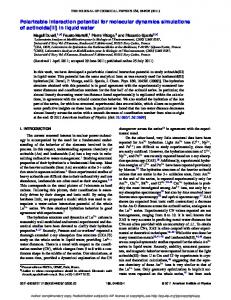
FIG. 13. (Color) NNDC nuclear binding data (greed circle), periodic table elements (black dots) vs. 𝐵𝐸𝑅𝐸𝐹 (purple line) The EIDIP Higgs boson energy was extracted from the 𝐵𝐸𝑟𝑒𝑓 magnitude scaling formula that the author has developed prior to the Higgs boson discovery. The equation (17) can be rewritten as

A. E-domain Interaction Constant (EIC) There are three types of E-domain Interaction Constants (EIC) for the rotational MWEP interaction: 𝑥 (1) 𝑌𝐸𝐼𝐶 = 𝑅03 for rotational MWEP interaction in Xdomains, 𝑐 (2) 𝑌𝐸𝐼𝐶 = 𝐻06 for rotational MWEP interaction in Cdomains.

0 𝐵𝐸𝑟𝑒𝑓 = [𝑃𝐸 × 𝐻𝑀𝑉 × R02 /(32π)]MeV

(18)

0 where 𝐻𝑀𝑉 is the EIDIP Higgs boson energy in 𝑀eV unit 0 𝐻𝑀𝑉 = [4𝜋𝐶 2 104 ]𝑀𝑒𝑉 ;

(19)

and the EIDIP Higgs boson mass in 𝑀eV/C 2 unit is B. Higgs boson mass and EIDIP nuclear binding energy model In the EIDIP nuclear binding energy (NBE) model, the EIDIP reference binding energy 𝐵𝐸𝑟𝑒𝑓 , which encloses known nuclei’s binding energy (purple curve, FIG. 13), was scaled from a normalized EIDIP (𝑃𝑒 ) 𝐵𝐸𝑟𝑒𝑓 = [𝑃𝐸 × (32𝜋)10−51 𝐻03 /2 × 𝐶 2 ]MeV

(16)

prior to the Higgs boson discovery on 2013 and it was later replaced by a simpler formula, which resulted only a 0.0086% higher scaling factor, 𝐵𝐸𝑟𝑒𝑓 = [𝑃𝐸 × 4𝜋104 R02 /(32π) × 𝐶 2 ]MeV

(17)

where R02 is the E-space isotropic membrane potential (EIMP) and (32𝜋) is the inter-domain mass factor (IMF). This 𝐵𝐸𝑟𝑒𝑓 equation indicate that the NBE unit is related to the spherical sheet of EIMP.

Or

0 𝐻𝑀𝐶 = [4𝜋104 ]𝑀𝑒𝑉/𝐶 2

(20)

0 𝐻𝑀𝐶 = [𝜇 1011 ]𝑀𝑒𝑉/𝐶 2

(21)

where 𝜇 is the vacuum permeability constant. Equation (19) gives a hint that Higgs boson mass, the source of mass, is related to a spherical sheet of EIMP. The EIDIP Higgs boson mass is [125.664]𝐺𝑒𝑣/𝐶 2 which compares with the measurements of ATLAS [126 ± 0.8]𝐺𝑒𝑣/𝐶 2 and CMS [125.3 ± 0.9]𝐺𝑒𝑣/𝐶 2 [2] [3]. The EIDI Higgs boson mass in kilogram unit (HigsKg 0 or 𝐻𝑘𝑔 ) is 0 0 𝐻𝑘𝑔 = [𝐻𝑀𝐶 × 1.7826 × 10−30 ]𝑘𝑔

(22)

where 1.7826 ∗ 10−30 is the standard 𝑀𝑒𝑣/𝐶 2 to kilogram conversion factor. V. EIDIP APPLICATION MODELS BRIEF This section contains brief description of EIDIP application models author have developed. For model detailed description, refer to individual EIDIP application model papers.

Copyrights (M.H.) 8/14/2014

Page 7/21

[email protected]

E-space Inter-Domain Interaction potential and fundamental forces

The EIDIP gravitational interaction model is the base of EIDIP application models and it can unify fundamental interactions. The gravitational interaction among objects has these elements: (1) MEGA: a Matter-Warped E-space Potential (MWEP) Gradient Induced Acceleration (MEGA), a Newtonian gravitational type acceleration; (2) SPGA: a Stationary EIDI Potential Gradient induced Acceleration (SPGA) among irrotational matters; (3) APIA: an EIDI Angular Potential (EIDIPr) Induced acceleration (APIA) among rotational matters. The MEGA magnitude in the non-saturated region is an inverse square function, whereas the SPGA and APIA are not; Both MEGA and APIA are always attractive at any distance; whereas the SPGA can be a negative attractive (repulsive) at short distance. The total gravitational interaction force consist of these three forces 𝐺𝑡𝑜𝑡𝑎𝑙 = (𝐺𝑀𝐸𝐺𝐴 + 𝐺𝑆𝑃𝐺𝐴 + 𝐺𝐴𝑃𝐼𝐴 );

(23)

Shown in FIG. 14, FIG. 15 and FIG. 16 are short range 𝐺𝑆𝑃𝐺𝐴 , short range 𝐺𝑆𝑃𝐺𝐶 and long range 𝐺𝑆𝑃𝐺𝐶 curves 4 associated with 𝑇𝑓𝑥𝐹 = √32𝜋; In this example, the 𝐺𝑆𝑃𝐺𝐴 has these characteristics (1) The short range 𝐺𝑆𝑃𝐺𝐴 is not an inverse square function and. At smaller separations the 𝐺𝑆𝑃𝐺𝐴 is repulsive (positive); (2) Over a very short range, the 𝐺𝑆𝑃𝐺𝐴 is highly attractive (negative); (3) Further away, the 𝐺𝑆𝑃𝐺𝐴 strength diminishes to small value close to an inverse square function (the 𝐺𝑆𝑃𝐺𝐶 settles to a constant) shown as a flat line portion of 𝐺𝑆𝑃𝐺𝐶 curve in FIG. 40. 50 SPGAEPd:TfxF=3.1665

40

EPdmin:-12.7658 [email protected]

30

GSPGA [x]

A. EIDIP Gravitational Interaction model

alternatively it can be expressed in inverse function form like Newtonian gravity formula as 𝐺𝑡𝑜𝑡𝑎𝑙 = (𝐺𝑀𝐸𝐺𝐶 + 𝐺𝑆𝑃𝐺𝐶 + 𝐺𝐴𝑃𝐼𝐶 )/𝑅2 where

EPdmax :45.8705 20

10

0

-10

𝐺𝑀𝐸𝐺𝐶 = 𝐺𝑀𝐸𝐺𝐴 × 𝑅2 ;

(24)

0

2

4

6

8

10

12

Radius [DSU]: R*2 dsu

𝐺𝑆𝑃𝐺𝐶 = 𝐺𝑆𝑃𝐺𝐴 × 𝑅2 ;

(25)

𝐺𝐴𝑃𝐼𝐶 = 𝐺𝐴𝑃𝐼𝐴 × 𝑅2 ;

(26)

FIG. 14. (Color) Short range 𝐺𝑆𝑃𝐺𝐴 associated with 4 𝑇𝑓𝑥𝐹 = √32𝜋 . 20

EPd*R2min:-72.3981

0

MWEP Gradient induced Acceleration

As shown in equations (6) and E-domain description in section II. D, the MWEP is an inverse function in the radius longer than two DSU region where the MWEP gradient induces a Newtonian type acceleration with the 𝐺𝑀𝐸𝐺𝐶 = [2R0 ]m3 /s2 as the EIDIP gravity constant.

GSPGC [x]

1.

SPGCEPd*R2:TfxF=3.1665

10

are the reconstituted MEGA , SPGA , and APIA gravitational interaction constants respectively.

-10

EPd*[email protected]

-20

EPd*R2max :16.5481

-30

EPd*R2max @0.683908 SPGCPdR2:Last:-52.2029

-40 -50 -60 -70 0

2

4

6

8

10

12

Radius [DSU]: R*2 dsu

2.

EIDIP gradient Induced Acceleration

Among irrotational matters, the gradient of EIDIP 𝑃𝑑 , a vector field, induces an attractive or repulsive force depends on the distance as shown in FIG. 14. The GSPGA can be expressed by this general formula: 𝐺𝑆𝑃𝐺𝐴 = 𝑀𝑠 𝑃𝑑 𝐻0 𝑅0 2 𝐹𝐼𝑀 𝐶 2

FIG. 15. (Color) Short range 𝐺𝑆𝑃𝐺𝐶 associated with 4 𝑇𝑓𝑥𝐹 = √32𝜋 .

(27)

where 𝑀𝑠 is the source mas, 𝐻0 is the Higgs boson mass, 𝑅0 2 is the EIMP, 𝐹𝐼𝑀 is the inter-domain mass factor, and 𝐶 is the speed of light.

Copyrights (M.H.) 8/14/2014

Page 8/21

[email protected]

E-space Inter-Domain Interaction potential and fundamental forces

10

60 SPGCEPd*R2:TfxF=3.1665

0

SPGCPdR2:Last:-49.8787

50

EIDIPr DSUEPr*1

GSPGC [x]

-10 -20 -30 -40

40

30 EIDIPrEPr:TfxF=3.1665

20

EPrmax :59.3412

-50

-70

EPrmax @2.15939

10

-60

-10

-5

10

10

0

0

10

EIDIPrPr:Last:51.0019 0

2

Distance [meter]: R*2 Rn0

FIG. 16. (Color) Long range 𝐺𝑆𝑃𝐺𝐶 associated with 4 𝑇𝑓𝑥𝐹 = √32𝜋 .

6

12

55 50 45 40 35 30

SPGAEPr:TfxF=3.1665

25

The EIDI Angular Potential (EIDIPr or 𝑃𝑟 ) induced acceleration ( 𝐺𝐴𝑃𝐼𝐴 ) can be expressed by this general formula:

(1) The 𝐺𝐴𝑃𝐼𝐴 is not a inverse square function and is always attractive (positive); (2) In short range, the 𝐺𝐴𝑃𝐼𝐴 decreases its strength with distance (asymptotic freedom behavior); (3) The 𝐺𝐴𝑃𝐼𝐴 fast raising prior the domain boundary and peaks around the reference E-domain boundary (2𝐷𝑆𝑈 ); (4) At further distance, the 𝐺𝐴𝑃𝐼𝐴 descends slowly and settle to a constant value (color confinement behavior); note that the normalized constant value (49.8593) is close to a complementary value of the normalized long range 𝐺𝑆𝑃𝐼𝐶 value of -49.8787 shown in FIG. 16.

SPGAPr:Last:49.8593

20 15

-10

10

-5

10

0

10

Radius [DSU]: R*2 Rn0

(28)

where 𝑀𝑠 is the source mas, 𝐻0 is Higgs boson mass, and 𝛿 is the inclination angle to reference matter equator. Shown in FIG. 17 is a 𝐺𝐴𝑃𝐼𝐴 associated with 𝑇𝑓𝑥𝐹 = 4 √32𝜋; In this example, the 𝐺𝐴𝑃𝐼𝐴 has these characteristics:

Copyrights (M.H.) 8/14/2014

10

60

GSPGA [x]

EIDI angular potential Induced acceleration

𝐺𝐴𝑃𝐼𝐴 = 𝑀𝑠 𝑃𝑟 𝐻0 𝐹𝐼𝑀 𝑌𝐸𝐼𝐶 𝐶 2 𝑐𝑜𝑠(𝛿) ;

8

FIG. 17. (Color) Short range 𝐺𝐴𝑃𝐼𝐴 function.

In the subatomic level, the 𝐺𝑆𝑃𝐺𝐴 engenders the residual strong force; in the molecule level, the 𝐺𝑆𝑃𝐺𝐴 engenders the inter-molecule short-range covalent bonding interactions; in the meter range the 𝐺𝑆𝑃𝐺𝐴 is part of gravity force and the source of Coulomb force as summarized in TABLE II. 3.

4

RDSU R*2*1;Mxp:2.15939;Mxv:59.3412

FIG. 18. (Color) Long range 𝐺𝐴𝑃𝐼𝐴 function. 𝑥 There are two type of APIA: in X-domains, a 𝐺𝐴𝑃𝐼𝐴 𝑥 3 which includes the expansionary 𝑌𝐸𝐼𝐶 = 𝑅0 ; and in C𝑐 𝑐 domains, a 𝐺𝐴𝑃𝐼𝐴 which includes the contractive 𝑌𝐸𝐼𝐶 = 6 𝑐 𝐻0 . The 𝐺𝐴𝑃𝐼𝐴 is tens order magnitude stronger than the GxAPIA due to the high magnitude order ratio between the 𝑐 𝑥 contractive and the expansionary EIC ( 𝑌𝐸𝐼𝐶 /𝑌𝐸𝐼𝐶 = 62 7.494 × 10 ). 𝑥 In the meter range the 𝐺𝐴𝑃𝐼𝐴 can be ignore due to the 𝑥 strength of the 𝐺𝐴𝑃𝐼𝐴 is tens order of magnitude weaker than the GMEGC (𝐺𝑀𝐸𝐺𝐶 /𝐺𝐴𝑃𝐼𝐶 > 1.8 × 1027 ). However at an inter-planet distance, combine with the source planet mass and the long range distance-independent behavior of 𝑥 the 𝐺𝐴𝑃𝐼𝐴 , it becomes noticeable. For example, the Pioneer space craft sunward acceleration anomaly and Milky Way 𝑥 rotational curve anomaly is engendered from the 𝐺𝐴𝑃𝐼𝐴 . At meter range, the Coulomb potential is dominated by the GSPGA ; however at Bohr radius, due to the high orbiting speed of electron, this centripetal force is mainly from the 𝑐 𝐺𝐴𝑃𝐼𝐴 induced force. At the subatomic range, combine with high magnitude 𝑐 𝑐 of the 𝑌𝐸𝐼𝐶 , the 𝐺𝐴𝑃𝐼𝐴 become several order magnitude stronger than the 𝐺𝑀𝐸𝐺𝐶 and produces the strong interaction.

Page 9/21

[email protected]

E-space Inter-Domain Interaction potential and fundamental forces

The Newtonian type gravitational constant 𝐺𝑀𝐸𝐺𝐴 is an 𝑥 inverse function; whereas 𝐺𝐴𝑃𝐼𝐴 , although much weaker in strength, remind almost constant at distance. At distance 𝑥 around 𝑅𝑥𝑂𝑣𝑒𝑟 = [23.67]𝑃𝐶 = [23.853]𝑅𝑥4 , the 𝐺𝐴𝑃𝐼𝐴 surpasses the 𝐺𝑀𝐸𝐺𝐶 . For example, at inter-galactic 𝑥 distance, the 𝐺𝐴𝑃𝐼𝐴 becomes the dominated force and produces those galaxy rotational velocity curve “anomalies”. 5.

The culprits in the gravitational interaction anomalies

The gravity interaction has multiple components, 𝐺𝑀𝐸𝐺𝐴 , 𝐺𝑆𝑃𝐺𝐴 and 𝐺𝐴𝑃𝐼𝐴 . The Newtonian gravity model lacks 𝐺𝑆𝑃𝐺𝐴 and 𝐺𝐴𝑃𝐼𝐴 components; and these missing components, especially the 𝐺𝐴𝑃𝐼𝐴 , is the culprits in the gravity interaction anomalies: (1) At the Dc0 domain boundary distance, the 𝐺𝑆𝑃𝐺𝐴 is highly attractive (red dash line in FIG. 14) and induced the large variance in Newtonian gravity constant measurements; (2) Although in the meter range, the 𝐺𝐴𝑃𝐼𝐴 can be neglected, at the inter-planet distance, with the heavy mass of source planet and the fast raising prior the domain boundary behavior, the 𝐺𝐴𝑃𝐼𝐴 become noticeable; which is the source of the Pioneer space craft sun-ward acceleration “anomaly”; (3) At some inter-galaxy distance, with the settle-toconstant at long distance behavior, the 𝐺𝐴𝑃𝐼𝐴 surpasses the 𝐺𝑀𝐸𝐺𝐴 and engenders the Milky Way rotation velocity “anomaly”. 6. Source of dark energy, dark matter and latest long range angular momentum boson The gravity interaction has multiple components, 𝐺𝑀𝐸𝐺𝐴 , 𝐺𝑆𝑃𝐺𝐴 and 𝐺𝐴𝑃𝐼𝐴 . The Newtonian gravity model lacks 𝐺𝑆𝑃𝐺𝐴 and 𝐺𝐴𝑃𝐼𝐴 components; in addition, the conventional Columbus force employs an inverse square distance function regardless the distance. The “dark” energy/matter were created to fit the observed data; Lately there are some paper propose a long range momentum boson (LRMB) to explain some astronomical mysteries and new dark energy for sub-atomic interactions. The 𝐺𝑆𝑃𝐼𝐴 and 𝐺𝐴𝑃𝐼𝐴 interaction components could make these dark energy/matter and the momentum boson creation unnecessary.

fits the rising segment, the anomaly acme distance and the slow descending segment (𝐺𝑆𝑊𝐴𝐴 , FIG. 20) of [4]. Pio. SWAA[cm/s] EPr*SunM*Hkg*R0*(32pi)*102

𝑥 4. The 𝐺𝐴𝑃𝐼𝐴 and 𝐺𝑀𝐸𝐺𝐴 crossover radius

9 8 7 SWAAEPr:TfxF=3.1665

6

EPrmax :8.81931 5

EPrmax @21.8671

4

Rx1Rx2 earthRx1

3

mR0sunRx0Rx1

2 1 0

0

10

20

30

40

50

RkpcR*2*C/2*(32pi)2/AU;Mxp:21.8671;Mxv:8.81931

FIG. 19. (Color) EIDIP Pioneer 10/11 SWAA curve

EIDIP SWAA curve

Rx1

Rx2 Rx2 domain boundary @

[(32 )2 *C]m  [20.25]AU

FIG. 20. (Color) The EIDIP Pioneer 10/11 SWAA curve Vs. empirical data C. EIDIP Milky Way circular velocity anomaly model The Milky Way Circular Velocity (CV) anomaly is from the settle-to-constant at inter-galaxy distance behavior that is missing from the Newtonian gravity model. Assuming at the time of creation, the initial velocity was omnidirectional with same magnitude distribution in all directions, the average circular and radical velocities of all stars at the time of creation was zero. Since dynamics of stellar systems is dissipationless, the radii binned average circular velocity curve of those stars with zero initial radical velocity should trace the CV curve (≈ √𝜌 ∗ 𝐺𝐴𝑃𝐼𝐴 where 𝜌 is galactic radius). The EIDIP Milky Way reference circular velocity curve (blue line in FIG. 21) fits the zone averaged absolute circular velocity (purple line) of those 16146 stars listed in the CDS RAVE-DDR2 database [5].

B. EIDIP Pioneer 10/11 anomaly model The Pioneer 10/11 spacecraft sun-ward acceleration anomaly is from the 𝐺𝐴𝑃𝐼𝐴 induced acceleration that is missing from the Newtonian gravity model. With these magnitude and distance scaling formula listed in TABLE III, the EIDIP Pioneer 10/11 acceleration anomaly curve

Copyrights (M.H.) 8/14/2014

Page 10/21

[email protected]

E-space Inter-Domain Interaction potential and fundamental forces

80

(0.2 kpc binned)

60

EIDIP reference CV

40

400

20 0

300

-20 200

-40 -60

100

 R * 4 Rn 0 / A

-80 Sun galactic radius

5

10

15

20

FIG. 23. (Color) inter-molecule potential curve overlaid on tip 2 IMP figure of [6].

-100

Galactic radius[kpc]

FIG. 21. (Color) RAVE-DDR2 mean CV (purple line) and EIDIP CV (blue line) curves. In galaxy’s outer region where 𝐺𝐴𝑃𝐼𝐴 ≫ 𝐺𝑀𝐸𝐺𝐴 , stars’ mean CV is a square root function of galactic radius. In this 𝐺𝐴𝑃𝐼𝐴 dominated region, the stars with longer the galactic radius would have higher circular velocity but lower angular velocity 𝑤 = √𝜌 ∗ 𝐺𝐴𝑃𝐼𝐴 /𝜌. Given enough time, these stars would form a spiral galaxy in this region. D. EIDIP inter-molecule potential model The inter-molecule potential (IMP) is a 𝐺𝑆𝑃𝐼𝐴 induced potential in inter-molecule distance. FIG. 23 depicts an EIDIP IMP model simulation overlays on an empirical figure of [6] (tip 2: smaller R tip) that depicts the interaction stiffness due to short-range covalent bonding interactions obtained by subtracting the long-range van-der-Waals background and correcting for the relaxation of tip and surface. The empirical figure’s distance axis includes some unknown offset “for the fact that the absolute zero of the distance axis is unknown”. With distance scaling factor 4𝑅0 𝑚 = 4 𝐷𝑆𝑈𝐷𝑐0 , the EIDIP inter-molecule potential curve (purple dash line) traces the empirical data mean curve. 30

FIG. 25 depicts an EIDIP IMP model simulation overlays on an empirical figure of [6] (tip 1: larger R, blunter); in this empirical figure, the distance axis is rescaled to account for the “the relaxation of the outermost tip atoms”. The EIDIP IMP curve (purple dash line) traces the empirical data mean curve. 5

IMF[Nm-1]EPd*Hkg*C3/4/6

0

IMF[Nm-1]EPd*Hkg*C3/4

EIDIP Inter-Molecule Potential curve (4DSU Scaled)

Dev. < CV unc.

|Circular velocity| [km/s]

500

RAVE-DDR2 Mean CV

Dev. > CV unc.

100 600

4

IMP1EPd:TfxF=3.1665

3

EPdmin:-3.21028 [email protected]

2

IMP1Pd:Last:-0.0920521

1 0 -1 -2 -3 -4

0

5

10

15

RAmR*2*R0*4*1010;Mnp:2.73225;Mnv:-3.21028

FIG. 24. (Color) EIDIPr IMP curve for tip 1 IMP figure of [12].

IMP2EPd:TfxF=3.1665 EPdmin:-19.2718

20

[email protected] IMP2Pd:Last:-0.000515262

10

EIDIP Inter-Molecule Potential curve (8DSU Scaled)

0

-10

 R * 8 Rn 0 / A -20 0

5

10

15

20

FIG. 25. (Color) IMP curve (purple dash line) overlaid on tip 1 IMP figure of [6].

25

RAmR*2*R0*2*1010;Mnp:1.36419;Mnv:-19.2718

FIG. 22. (Color) EIDIPr inter-molecule potential curve for tip 2 IMP figure of [6].

E. EIDIP strong force and nuclear force model The strong force is a 𝐺𝐴𝑃𝐼𝐴 induced force in sub-atomic range; whereas the nuclear force (neutron-neutron

Copyrights (M.H.) 8/14/2014

Page 11/21

[email protected]

E-space Inter-Domain Interaction potential and fundamental forces

Strong force [Newton]

10000 Long range SF ≈ 9814.98 Newton

8000

EIDIP Strong Force curve

6000

2 2

2

3

EPd*Nm *HgMc*R0 /(32pi) *C

12000

listed in TABLE III, the EIDIP nuclear force curve phenomenological fits the ECP curves of AV18 and Reid93 from [9] as shown in FIG. 29.

NN potential [Mev]

potential) is a 𝐺𝑆𝑃𝐼𝐴 induced force. As shown in FIG. 26, the EIDIP Strong Force curve depicts the strong interaction asymptotic freedom behavior at short range and a settle to constant color confinement behavior at long range. With these magnitude and distance scaling formula listed in TABLE III, the Long range EIDIP SF strength (~9814.98) matches the empirical long range strong interaction strength ~9800 Newton of matches the empirical long range strong interaction strength ~9800 Newton from “the Behavior of the strong force” [7].

4000

2000

0

-2

SFmaxR

500

Repulsive region

400 300

EIDIP NN potential curve

200

100

Highly attractive region

0 -100 -200

MNPmaxR@ 0.67408 fm 0

0.5

R

1

1.5 2.5

2 15

fm R*2*R0/(32pi) *10

;

2.5

3

3.5

4

Mnp:0.674079;Mnv:-137.902

FIG. 28. (Color) EIDIP NN potential (1S0) curve.

Asymptotic freedom behavior

10

600

SFmaxR@ 0.7073 fm 0

2

10

10

4

10

Radius [fm]: R*2Rn2.5*1015

FIG. 26. (Color) EIDIPr Strong force curve. The normalized EIDIP strong force (purple dash line) phenomenological fit to the QCD base effective strong coupling constants (ESCC) figure (FIG. 27) [8, p. 35]. Normalized EIDIP Strong Force curve EIDIP NN potential

r[fm]

FIG. 29. (Color) AV18 Reid93 and EIDIP NN potential curve (blue dash line). With these distance scaling formula listed in TABLE III, The EIDIP strong force curve acme radius 0.7073 fm (𝑆𝐹𝑚𝑎𝑥𝑅) and the EIDIP nuclear force curve yielded a maximum nuclear attraction force radius, 𝑅𝑁𝑁𝑃𝑚𝑎𝑥 = 0.67408 𝑓𝑚 . Both radius were also indirectly verified through the 885 (A>16) nuclei empirical nuclear charge radius data set and in EIDIP neutron, proton, and hydrogen Isotope 2𝐻11 NCR formulas SFmaxR@ 0.7073 fm

FIG. 27. (Color) EIDIP ESCC Vs. QCD base ESCC curve.

F. EIDIP electrical force and Bohr radius model

As shown in FIG. 28, the EIDIP nuclear force (NN potential) curve depicts that the residual strong force is repulsive at short distance behavior and is highly attractive behavior at between 0.5-2 fm. With these magnitude and distance scaling formula

There are two type of electrical forces: an EIDIP Coulomb force induced from an 𝐺𝑆𝑃𝐼𝐴 induced force, and a centripetal force from 𝐺𝐴𝑃𝐼𝐴 induced force. The 𝐺𝑆𝑃𝐼𝐴 type force dominate the interaction between irrotational charges and is close to an inverse square distance function in longer than 10−8 meter range; whereas the 𝐺𝑆𝑃𝐼𝐴 type of force

Copyrights (M.H.) 8/14/2014

Page 12/21

[email protected]

E-space Inter-Domain Interaction potential and fundamental forces

dominate the interaction for those high orbiting speed electrons. For example, the centripetal force of high orbiting speed electron at Bohr radius is mainly from 𝐺𝑆𝑃𝐼𝐴 induced force. The EIDIP Bohr Radius is the maximum magnitude radius of a 𝐺𝑆𝑃𝐼𝐴 induced force. With the distance scaling formula listed in TABLE III, the electron centripetal force curve peak at 5.27746 E-11 m (FIG. 30) which compares with the CODATA Bohr Radius of 5.2917721092(17)E-11 m

(3) The conventional Columbus force is an inverse square distance function regardless the distance; whereas at short distance, the 𝐺𝑆𝑃𝐺𝐶 portion of EIDIP Columbus force is not an inverse square distance function. The author congests that this short range Columbus function deviation resulted the rounder curve in the maximum negative charge area of empirical NCD curve. 60

Normalized EIDIP unit

Electric force [Pr unit]

60 50 40 30 20

EPrmax @52774.6

2

3

4

6

Distance [fm]: R*2 Rn0*1015

7

-40

Nuclear force portion of NCD

Neutron “positive” charge region

8 4

x 10

FIG. 30. (Color) EIDIP Bohr Radius curve. G. EIDIP neutron charge distribution curve indicates EIDIP can unify the fundamental forces A preliminary EIDIP neutron charge distribution (NCD) model is good indicator that the EIDIP can unify the fundamental strong and Columbus forces. In the EIDIP NCD model, the neuron “charge” distribution is engendered from the sum of the 𝐺𝐴𝑃𝐼𝐴 induced strong force and the 𝐺𝑆𝑃𝐺𝐴 induced nuclear force that has inverted effect on the negative charge electron projectile. These two type of forces constitute the electrical force rather than the conventional Columbus force that has an inverse square distance function regardless the distance. The third sub-figure of FIG. 31 depicts an aggregated Neuron Charge Distribution (NCD) from experiments that use polarization techniques in electron scattering [10]. As shown in the first sub-figure of FIG. 31, the EIDIP NCD curve (blue curve) is the sum of the EIDIP strong force curve and an inverse square distance reconstituted (𝐺𝑆𝑃𝐺𝐶 ) EIDIP nuclear force curve. The reason of using a reconstituted EIDIP nuclear force curve is to accommodate the conventional Columbus inverse square distance function that is used in “charge” distribution extraction from experimental data. As shown in FIG. 31, the EIDIP NCD curve compare with the mean curve of aggregated empirical NCD curve. In addition, note that (1) The min/max radius are closed aligned especially the acmes of EIDIP nuclear force curve and aggregated neutron charge distribution curve, and (2) Both have similar positive to negative range ratio.

Copyrights (M.H.) 8/14/2014

EIDIPr PdR2 (Pr+PdR2)

-20

50 5

Neutron Charge distribution

1

=Nuclear force + strong force

0

-80

BohrR:52917.7fm 0

EIDIP NCD curve

20

-60

BOHREPr:TfxF=100.53

10 0

Strong force portion of NCD

40

70

40 30

EIDIP NCD curve

20

Maximum positive charge to minimum negative charge ratio ~3

10

0

Neutron “negative” charge region

-10 -20

0

0.5

1

1.5

2

2.5

3

3.5

4

Distance [fm]: R*2 Rn2.5 *1015

Maximum positive charge to minimum negative charge ratio ~3

Aggregated empirical NCD mean curve

FIG. 31. (Color) EIDIP neutron charge distribution + strong interaction curve. EIDIP NCD curve (blue curve); EIDIP strong force curve (red curve in the first subfigure); EIDIP inverse square distance reconstituted nuclear force curve (light green curve) The EIDIP NCD curve can model the positive and negative “charge” distribution; since the “charge” is the source of the Columbus force, the EIDIP NCD curve indicates that the EIDIP can unify the fundamental gravity, strong force and Columbus forces.

Page 13/21

[email protected]

E-space Inter-Domain Interaction potential and fundamental forces

H. EIDIP interaction model summary tables TABLE II. EIDIP application model EIDIP SPGA and APIA magnitude transformation formulas. App. Model

EIDIP magnitude transformation formula (partial) 2.5 ]IMF

∗ GxAPIA ]m/(kg∗s2 ).

Milky Way RC

[[(32π)

Pioneer anomaly

[[1/(32π)]IMF Rx1/Rx2

Fly By anomaly

[[C/2]IMF Rx0/mR0

∗ GxAPIA ]

∗ GxAPIA ]

m/(kg∗s2 )

m/(kg∗s2 )

.

Bohr Radius

[[(32π)]IMF Dc0/ Dc1 ∗ GcAPIA ]

Strong force

[[(32π)3 ]IMF Dc0/ Dc3

Covalent force

N [[C]IMF mR0/ Dc0 ∗ GSPGA /4]

Nuclear force

Mev [[1/(32π)3 ]IMF Dc3/ Dc0 ∗ GSPGA ]

Gravity (SPGA)

[[H0 ]IMF mR0/ Dc0

Binding energy

[[1/(32π)]IMF Dc3/ Dc2

∗

m/(kg∗s2 )

∗ GcAPIA ]

.

m/(kg∗s2 )

m/(kg∗s2 )

.

.

Mev

.

N GSPGA /C 2 ] . m/(kg∗s2 ) Mev ∗ GSPGA ∗ 2]

Mev

.

.

TABLE III. EIDIP application model distance and magnitude transformation formulas. App. Model

Distance scaling factor

Magnitude scaling formula

Milky Way RC anomaly

[(32π)5 ∗ C]m = [2]DSU Rx5

[𝑃𝑟 ∗ 𝑀𝑀𝑊𝑆 ∗ 𝐻𝑘𝑔 ∗ [(32π)2.5 ]𝐼𝑀𝐹 ∗ [𝑅0 ]

Pioneer 10/11 anomaly

[(32π)2

Near Earth Fly By anomaly

[C]m = [2]DSU Rx0

∗ C]m =

[2]DSU Rx2

Remark

0

[𝑃𝑟 ∗ 𝑀𝑠𝑢𝑛

3

xEIC

0 3 ∗ 𝐻𝑘𝑔 ∗ [1/(32π)]𝐼𝑀𝐹 ∗ [𝑅0 ]

m/s

3

[𝑃𝑟 ∗ 𝑀𝑚𝑜𝑜𝑛 ∗ 𝐻𝑘𝑔 ∗ [C/2]𝐼𝑀𝐹 ∗ [𝑅0 ]

𝑀𝑠𝑢𝑛 : estimated sun mass;

∗C ]

m/s2

𝑀𝑚𝑜𝑜𝑛 : estimated moon

∗ C2]

xEIC

m/s

mass;

0 [𝑃𝑑 ∗ 𝐻𝑘𝑔 ∗ [𝐻0 ]𝐼𝑀𝐹 ]

[2]DSU Dc0

Gravity (GSPGA)

[2𝑅0 ]m =

Covalent force

[2𝑅0 ]m = [2]DSU Dc0

0 [𝑃𝑑 ∗ 𝐻𝑘𝑔 ∗ [C/2]𝐼𝑀𝐹 ∗ C 2 /2]

Bohr Radius

[2𝑅0 ]m = [2]DSU Dc0

[𝑃𝑟 ∗ 𝑚𝑒 ∗ 𝑚𝑝 ∗ 𝐻𝑘𝑔 /2 ∗ [1/(32π)2.5 ]𝐼𝑀𝐹 ∗ [𝐻0 ]

Strong force

[2𝑅0 /(32π)2.5 ]m = [2]DSU Dc2.5

[𝑃𝑟 ∗

2 𝑚𝑢𝑞,𝑘𝑔

NN potential

[2𝑅0 /(32π)2.5 ]m

[2]DSU Dc2.5

[𝑃𝑑 ∗

2 𝑚𝑛,𝑀𝑒𝑣 ⁄𝐶 2

Ref. binding energy

[2𝑅0 /(32π)2 ]m

m/(kg∗s2 )

1/2 factor is case dependent

kg/s2

0

6

∗ C2]

cEIC

=

=

[2]DSU Dc2

0 [𝑃𝑒 ∗ (𝐻𝑀𝐶

0 6 ∗ 𝐻𝑘𝑔 ∗ [(32π)3 ]𝐼𝑀𝐹 ∗ [𝐻0 ]

N

cEIC

𝑅20 ) ∗ [1/(32π)]𝐼𝑀𝐹 ∗ C2 ]

Mev

Statistical significance is a statistical assessment of whether observations reflect a pattern rather than just chance. The fundamental challenge is that any partial picture of a given hypothesis is subject to random error. In statistical testing, a result is deemed statistically significant if it is so extreme that such a result would be expected to arise simply by chance only in rare circumstances. Hence the result provides enough evidence to reject the hypothesis of 'no effect'. In nuclear and particle physics, it is common to express statistical significance in units of the standard deviation of a normal distribution [11]. Three section of Null Hypothesis Test Nodes (NHTN) extracted from EIDIP application models are created to calculate the EIDIP’s confidence level. Each NHTN contains a finding from EIDIP model simulation and empirical data comparison. A null-hypothesis is set as “a 0.5 probability that this result is coincidental (no effect)”. A "5 sigma confidence level” is that the likelihood of obtaining the experimental result by coincidence is 0.00005733%. In order for EIDIP to have 5 sigma confidence level, it will need 21 NHTNs to be all nulled (result of chance).

𝑚𝑒 and 𝑚𝑝 : electron and proton mass; 𝑚𝑢𝑞,𝑘𝑔 : up quark mass;

2

∗C ]

N

0 2 ∗ (𝐻𝑀𝐶 ∗ 𝑅0 ) ∗ [1/(32π)3 ]𝐼𝑀𝐹 ∗ C 2 ]

VI. EIDIP NULL HYPOTHESIS TESTING NODE LIST

Copyrights (M.H.) 8/14/2014

mass;

2

xEIC

0

𝑀𝑀𝑊𝑆 : Milky Way stellar

∗ C2 ]

Mev

𝑚𝑛,𝑀𝑒𝑣⁄𝐶 2 : neutron mass;; 0 𝐻𝑀𝐶 : EIDI Higgs boson mass;

A. Null Hypothesis Test Nodes section I (NHTN-I) NHTN’s in this section were extracted from those EIDIP application models that have been verified with large empirical numerical data sets. (1) The EIDIP based 𝐵𝐸𝑅𝐸𝐹 (purple curve, FIG. 13) set the upper bound of nuclear binding energy (NBE) for known 2436 nuclei; deviation between AME NBE and 𝐵𝐸𝑅𝐸𝐹 is a parabola function as shown in FIG. 32. (2) The deviation between the NBE and the EIDIP reference NBE BEref is a parabola function which contributed to formulation of the more accurate yet simpler EIDIP NBE formula. Reference to the 2436 experimental NBE in the 2012 Atomic Mass Evaluation table (AME2012), the 𝐵𝐸𝑅𝐸𝐹 based NBE formula calculated data has 0.094 St. Dev. Vs. 0.415 St. Dev. of the liquid drop model based semi-empirical NBE formula (SEMF) [12];

Page 14/21

[email protected]

E-space Inter-Domain Interaction potential and fundamental forces

6

4

2

1

0

15

30

30

25

20

15

10

5

ber Proton num

FIG. 32. (Color) Deviation between AME NBE 𝐵𝐸𝑅𝐸𝐹 is a parabola function

(29)

0 𝐵𝐸𝑟𝑒𝑓 = [𝑃𝑒 ∗ 𝐻𝑀𝐶 R02 𝐶 2 /(32𝜋)]MeV .

(30)

[1/C 2 ]m/A

The distance transform factor 𝑅𝑢 = was used as the mass number to inter-nucleon reference distance conversion factor to lookup the 𝐵𝐸𝑟𝑒𝑓 in the EIDIP NBE calculation. Small alternation in this factor resulted rapid increase in St. Dev. of calculated NBE. The EIDIP to reference binding energy magnitude scaling factor include the isotropic E-space energy R02 unit.

EIDIP NCR baseline: CRb  A * R q  CR oft

R q  24 * Ru  24/C 2

3

2.5

0

50

100

150

200

250

Mass Number:A[16:248] FIG. 33. (Color) ENSEF produced NCR and ADND13A16 NCR on mass number axis. (6) The muonic hydrogen radius calculated from the EIDIP proton muonic NCR formula [14] yielded 0.842145 fm, which compares with the newer muonic hydrogen NCR measurement of [0.84184 ± 0.00067]fm ; the hydrogen charge radius calculated from the EIDIP proton NCR formula is 0.87705 fm, which compares with the CODATA 2006 proton charge radius [0.8768 ± 0.0069]fm [14], [0.879 ± 0.015]fm of [15], [0.895 ± 0.018]fm of [16], and [0.8737 ± 0.0075]fm of [17].

(4) The simplicity (2 domain spatial unit) of the EIDIP NBE model EIDIP distance to LBID transform formula:

Muonic proton NCR

(31)

(5) A nucleon Spherical shell Packing Radius (NSPR) based with the EIDIP semi-empirical nuclear charge radius formula (ENSEF) calculated nuclear charge radius (NCR) [1] matched 47.8% of those 885 (mass number ≥16) nuclei NCR listed in the 2013 Atomic Data and Nuclear Data Tables (ADND13-A16); which is better than 35.5% matches of a Skyrme-Hartree-Fock Bogoliubov (HFB) model based, with Weizs¨ackerSkyrme (WS) mass model refined, semi-empirical NCR formula (WSSEF) [13]. The ENSEF does not require WSSEF’s shell correction obtained from the traditional Strutinsky procedure; the simpler ENSEF yielded 0.0199 fm rms deviation, compares with 0.0218 fm rms of the WSSEF. FIG. 33 depicts the ENSEF produced NCR (red dots) overlay on the ADND13-A16 (blue dots).

Rq3 Rq4

𝑅𝐿𝐵𝐼𝐷 = 𝑅[2𝑅0 /(32𝜋)2 ]𝑚 = 𝑅[2]𝑅𝑛2 𝐷𝑆𝑈 .

4

3.5

(3) The low 0.094 St. Dev. affirms that the distilled Higgs boson mass from EIDIP to 𝐵𝐸𝑟𝑒𝑓 magnitude scaling, and the simple 𝐶 2 factor of the EIDIP distance to mass number (A) transform formula were not arbitrary [12] 𝑅𝑛2 2 𝐴 = [2]𝑅𝑛2 𝐷𝑆𝑈 𝐶 𝑅 = 𝑅 [2]𝐷𝑆𝑈 /𝑅𝑢 ,

4.5

SFmaxR

Rq5 3Ru4

10

Neutron 20 25 number

EIDIP NCR

u-

Radius

Projectile

FIG. 34. (Color) EIDIP proton muonic NCR components.

Electronic proton NCR SFmaxR

Rq4 3Ru

5

5

Rq3 Rq4

-1

ADND13 NCR

5.5

Nuclear Charge Radii [fm]

BEREF-BEAME12e

3

e-

Radius

FIG. 35. (Color) EIDIP proton electronic NCR components.

Copyrights (M.H.) 8/14/2014

Page 15/21

[email protected]

E-space Inter-Domain Interaction potential and fundamental forces

Account for the 𝑆𝐹𝑚𝑎𝑥𝑅 in the measured neutron NCR, the EIDIP neutron NCR formula yielded −0.114906 fm which matches the 𝑅11𝐻 = −0.1149 ± 0.0027 fm listed in the ADND13 table.

FIG. 38. (Color) EIDIP Milky Way RC model RAVE deviation over RAVE uncertainty range value. B. The Null Hypothesis Test Node list II (NHTN-II)

Measured neutron NCR =-0.1149 fm

The NHTN in this section are extracted from EIDIP application models’ simulations and empirical figures or small number of empirical data comparisons.

Neutron core

2Ru 3Ru Rq4

Rq3 Rq3

SFmaxR

Radius FIG. 36. (Color) EIDIP Neutron NCR components. The EIDIP hydrogen isotope 2𝐻11 NCR formula yielded 2.1419 fm which compares with the 2010 CODATA recommended 2.1424 ± 0.0021 fm and the 2.1421 ± 0.0088 fm listed in the ADND13 table.

Rq4 3Ru

Rq4 NNPmaxR Rq3 Rq4

Rq3 Rq3 2Ru 3Ru

hydrogen isotope NCR Neutron core Electronic proton NCR

SFmaxR

Radius

e-

FIG. 37. (Color) EIDIP 2𝐻11 NCR compositions. (7) The Circular Velocity (CV) anomaly and the spiral star distribution pattern can be explained by the missing GAPIA in the Newtonian gravity model without involving the “dark matter” as shown in in FIG. 21. (8) The simplicity (2 domain spatial unit) of the EIDIP Milky Way model distance transform factor (32𝜋)5 𝐶 𝑚 = 2 𝐷𝑆𝑈𝑅𝑥5 [18]. (9) The EIDIP Milky Way reference circular velocity curve intersects with 36.659% of the CDS RAVE-DDR2 16146 stars’ circular velocity range as shown in FIG. 38 (eUgap 16) nuclei empirical nuclear charge radius data set and in EIDIP neutron, proton, and hydrogen Isotope 𝟐𝑯𝟏𝟏 NCR formula [14]. (3) The Long range EIDIP SF strength (~9814.98) matches the empirical long range strong interaction strength ~9800 Newton from “the Behavior of the strong force” [7]. (4) The simplicity (2 domain spatial unit) of the EIDIP SF model EIDIPr distance to inter-nucleon distance transform factor [2𝑅0 /(32𝜋)2.5 ]𝑚 is two DSU of Ddomain 𝐷𝑐2.5 . (5) At long range, the EIDIP Strong Force curve (blue line, FIG. 26) depicts the strong interaction color confinement behavior. (6) At short range, the EIDIP Strong Force curve (FIG. 26) depicts the strong interaction asymptotic freedom behavior. (7) The EIDIP two-nucleon 1S0 Inter-nucleon potential model depicts the residual strong force is repulsive at short distance (FIG. 28); (8) The EIDIP two-nucleon 1S0 Inter-nucleon potential model depicts the residual strong force is highly attractive between 0.5-2 fm (FIG. 28). (9) The simplicity (2 domain spatial unit) of the EIDIP Inter-nucleon potential model distance scaling factor 2𝑅0 /(32𝜋)2.5 𝑚 = 2 𝐷𝑆𝑈𝑅𝑛2.5 . This distance scaling factor yielded a maximum nuclear attraction force radius, 𝑅𝑁𝑁𝑃𝑚𝑎𝑥 that was used in the EIDIP hydrogen Isotope 2 1 𝐻1 NCR formula as shown in FIG. 37 and yielded 2.1419 fm; which matches the 2010 CODATA recommended R 21H = 2.1424 ± 0.0021 fm and the R 21H = 2.1421 ± 0.0088 fm of the ADND13 table. (10) The EIDIP two-nucleon 1S0 Inter-nucleon potential (residual strong force) curve phenomenological fits the ECP curves of AV18 and Reid93 from [9] as shown in FIG. 29. (11) The EIDIP Neuron Charge Distribution (NCD) curve (the blue curve in first and second sub-figures in FIG. 31) is a sum of a subatomic range 𝐺𝐴𝑃𝐼𝐴 = 𝑓(𝑃𝑟 ) curve (strong force portion, the red curve in the first subfigure in FIG. 31) and 𝐺𝑆𝑃𝐺𝐶 = 𝑓(𝑃𝑑 × 𝑅2 ) curve (nuclear force portion, the light green curve in the first sub-figure in FIG. 31). The EIDIP NCD curve resembles the mean curve of aggregated NCD curve (black curve of

Page 16/21

[email protected]

E-space Inter-Domain Interaction potential and fundamental forces

Copyrights (M.H.) 8/14/2014

-13

x 10 1

SPGCEPd*R2:TfxF=3.1665 EPd*R2min:-4.88091e-013

GSPGC[m3/s2]

0

EPd*[email protected] -1

EPd*R2max :1.15265e-013 EPd*R2max @2.1946e-011

-2

SPGCPdR2:Last:-3.37153e-013 SPGCPdR2:min:-4.88091e-013

-3

-4

-5

-11

10

-10

10

-9

-8

10

10

Distance [meter]: R*2 Rn0

FIG. 39. (Color) An EIDIP atomic-range SPGC curve. (20) The EIDIP Gravitational interaction include 𝐺𝑀𝐸𝐺𝐴 , 𝐺𝑆𝑃𝐺𝐴 , and 𝐺𝐴𝑃𝐼𝐴 . The 𝐺𝑀𝐸𝐺𝐴 is the gradient of the MWE E-space potential (MWEP); interaction between two MWEP engenders the EIDIP. Both the 𝐺𝐴𝑃𝐼𝐴 and the 𝐺𝑆𝑃𝐺𝐴 are derived from the EIDIP. In the meter range, the sum of the 𝐺𝑀𝐸𝐺𝐶 and the retrofired 𝐺𝑆𝑃𝐺𝐶 constitutes 99.94% of 2010 CODATA-recommended gravitational 𝑁 𝑁 constant value G value [18], 𝐺𝑀𝐸𝐺𝐶 + 𝐺𝑆𝑃𝐺𝐶 = 6.66972 × 10−11 𝑚3 𝑘𝑔−1 𝑠 −2 . -13

2

x 10

29-Apr-2014 SPGCEPd*R2:TfxF=3.1665

GSPGC[m3/s2]EPd*R2*Hkg*H0

the third sub-figure in FIG. 31) from experiments that use polarization techniques in electron scattering [10]. These resemblances indicate that the EIDIP function can model the positive and negative “charge” distribution, and the electrical force. (12) The simplicity (2 domain spatial unit) of the EIDIP neuron charge distribution curve distance scaling factor 2𝑅0 /(32𝜋)2.5 𝑚 = 2 𝐷𝑆𝑈𝐷𝑐2.5 . (13) FIG. 23 depicts an EIDIP inter-molecule potential model simulation overlays on an empirical figure of [6] (tip 2: smaller R tip) that depicts the interaction stiffness due to short-range covalent bonding interactions obtained by subtracting the long-range van-der-Waals background and correcting for the relaxation of tip and surface. The empirical figure’s distance axis includes some unknown offset “for the fact that the absolute zero of the distance axis is unknown”. With distance scaling factor 4 𝐷𝑆𝑈𝐷𝑐0 , the EIDIP inter-molecule potential curve traces the empirical data mean curve. (14) The simplicity (4 domain spatial unit) of the EIDIP inter-molecule potential curve distance scaling factor 4𝑅0 𝑚 = 4 𝐷𝑆𝑈𝐷𝑐0 as shown in FIG. 22. (15) FIG. 25 depicts an EIDIP inter-molecule potential model simulation overlays on an empirical figure of [6] (tip 1: larger R, blunter); in this empirical figure, the distance axis is rescaled to account for the “the relaxation of the outermost tip atoms”. The EIDIP inter-molecule potential curve (purple dash line) traces the empirical data mean curve. (16) The simplicity (8 domain spatial unit) of the EIDIP inter-molecule potential model distance scaling factor 8𝑅0 𝑚 = 8 𝐷𝑆𝑈𝐷𝑐0 as shown in FIG. 24. (17) EIDIP electrical force model hypothesizes that there are two type of electrical forces: an EIDIP Coulomb force induced from an EIDIP gradient (𝑃𝑑 ) induced force, and a centripetal force from an EIDI angular potential (𝑃𝑟 ) induced force that is acting on the high orbiting speed electron at the Bohr radius. As shown in FIG. 30, with [2𝑅0]𝑚 distance scaling factor, the EIDIPr peak at 5.2944 E-11 m which compares with the CODATA Bohr Radius of 5.2917721092(17)E-11 m. (18) The simplicity (2 domain spatial unit) of the EIDIP Bohr Radius curve EIDIPr distance transform factor [2R 0 ]m = 2 𝐷𝑆𝑈𝑅𝑛0 . (19) The reconstituted 𝐺𝑆𝑃𝐺𝐶 = 𝐺𝑆𝑃𝐺𝐴 𝑅2 (blue line) is not an inverse square function as shown in FIG. 39 and can explain the contradictories among the Newtonian gravitational constant measurements [18].

EPd*R2min:-3.36728e-013

1

EPd*[email protected]

0

EPd*R2max :6.60335e-014 -1

SPGCPdR2:Last:-3.36728e-013 Rn0 mR0

-2 -3 -4 -5

-10

10

-5

10

0

10

RmR*2*R0;Mnp:38.1865;Mnv:-3.36728e-013

FIG. 40. (Color) An EIDIP gravity 𝐺𝑆𝑃𝐺𝐶 curve. (21) The EIDIP Pioneer 10/11 acceleration anomaly curve phenomenological fits the rising segment, the anomaly acme distance and the slow descending segment (𝐺𝑆𝑊𝐴𝐴 , FIG. 20) of [4]. Recent paper (arXiv:1204.2507) [19] concluded that, after account for all thermal recoil forces (TRF) including source uncertainty, no statistically significant acceleration anomaly exists. The overlap coefficient is a similarity measure related to the Jaccard index that is a statistic used for comparing the similarity and diversity of sample sets. If set X is a subset of Y or the converse then the overlap coefficient is equal to one. The overlap coefficient of ((ηelec , ηrtg ) between the TRF analysis model generated data set and the measured Doppler residual data set is around 20% which indicates low similarity between these two sets and that the

Page 17/21

[email protected]

E-space Inter-Domain Interaction potential and fundamental forces

proposed TRF model has low probability to be the Pioneer anomaly. Refer to appendix section for TRF Vs. 𝐺𝑆𝑊𝐴𝐴 model comparison. (22) The simplicity (2 domain spatial unit) of the EIDIP Pioneer 10/11 anomaly EIDIPr distance transform factor (32𝜋)2 𝐶 𝑚 = 2 𝐷𝑆𝑈 of Rx2 E-space domain. C. The Null Hypothesis Test Node list III (NHTN-III) Supporting or cross models NHTNs from EIDIP application models’ empirical figure/data comparisons. (1) The EIDIP Higgs boson mass is [125.664]𝐺𝑒𝑣/𝐶 2 is within the ATLAS (126 ± 0.8 𝐺𝑒𝑉 𝐶 −2 ) [3] and CMS’s 125.3 ± 0.9 𝐺𝑒𝑉 𝐶 −2 [2] Higgs Boson mass range. (2) 𝑖𝑀𝑢 is the EIDI Interaction Mass defect unit used in the EIDIP magnitude transform formula in the EIDIP nuclear binding energy model prior to the Higgs boson discovery [12]. 𝑖𝑀𝑢 = [(32𝜋)2 10−51 𝐻05 /2]𝑀𝑒𝑉/𝐶 2 ;

(32)

earth fly-by pass showed a speed “anomaly” and other fly-by passes did not [20]. (11) The EIDIP angular potential induced GAPIA (refer to equations in V. A.3) can unify the strong interaction at the subatomic distance and the gravitational interaction “anomalies” at the inter-planet or interstellar distance as shown in TABLE II. (12) The EIDIP gradient induced GSPGA (refer to equations in V. A.2) can unify the gravitational interaction, the inter-nucleon potential, and inter-atomic potential as shown in TABLE II. (13) The shared components of magnitude transform formulas among EIDIP application models: Higgs Boson mass, 32π IMF factors, and EIDIP constant R0 as shown in “magnitude scaling factor” column of TABLE III. (14) The commonality and the simplicity of the Domain Spatial Unit (DSU) based distance transform formulas used among the EIDIP application models as shown in “distance scaling factor” column in TABLE III. VII.

EIDIP FUNCTION 5+CONFIDENCE LEVEL POTENTIAL

Which was later replaced by a simpler formula (resulted only 0.0086% higher value) 𝑖𝑀𝑢 = [4𝜋104 ]𝑀𝑒𝑉/𝐶 2

A. Discovery standard and sigma confidence level (33)

or with EIDIP Higgs Boson mass formula 0 𝑖𝑀𝑢 = [𝐻𝑀𝐶 × 𝑅02 /(32𝜋)]𝑀𝑒𝑉/𝐶 2

(34)

(3) The EIDIP SF model EIDIPr magnitude transform 0 formula includes the EIDI Higgs boson mass (𝐻𝑘𝑔 ) and the Long range EIDIP SF strength (~9814.98 as shown in FIG. 26) matches the empirical long range strong interaction strength ~9800 Newton from “the Behavior of the strong force” [7]. (4) The EIDIP reference NBE formula EIDIP magnitude transform formula includes the EIDI Higgs boson mass (refer to TABLE III); (5) The Inter-nucleon potential curve magnitude transform formula includes the EIDI Higgs boson mass. (6) The inter-molecule potential curves magnitude transform formula includes the EIDI Higgs boson mass; (7) The EIDIP Pioneer 10/11 anomaly curve EIDIPr magnitude transform formula includes the EIDI Higgs boson mass [18]; (8) The EIDIP Milky Way reference circular velocity formula includes the EIDI Higgs boson mass; (9) The EIDIP nuclear charge radius model includes an quantized lower bound inter-nucleon distance unit (𝑅𝑢 ) nucleon shell radius gradient unit [14]: 𝑅𝑁𝐶𝑏 = 24𝑅𝑢 √𝐴 + 𝑅𝑁𝐶𝑜𝑓𝑡 .

(35)

(10) The moon mass induced GxAPIA to the NEAR flyby anomaly phenomenological data fit at the perigee and can also explain why, for a same satellite, one near

Copyrights (M.H.) 8/14/2014

A "3 sigma confidence level” is equivalent to saying that the likelihood of obtaining the result by coincidence is 0.26998%; whereas A "5 sigma confidence level” is that the likelihood of obtaining the experimental result by coincidence is 0.00005733% or one in 1,744,277.9 cases. In nuclear and particle physics, the 3 sigma confidence level is the “preliminary discovery” standard that deserved further investigation; whereas the 5 sigma confidence level is the golden “discovery” standard. B. EIDIP confidence level If we set null-hypothesis as “each null hypothesis testing nodes has 0.5 probability that the result is coincidental and has no relationship with the EIDIP function, the test target”. (1) The chance of the 9 NHTNs in the section I are all true (Just coincidental) is 0.59 , which is lower than 0.27027%, the 3 sigma confidence level threshold. The section I NHTN alone indicates a 3+ sigma confidence level for the EIDIP function. 1) The chance of the 9+22 NHTNs in the section I and II are all true (Just coincidental) is 0.531 , which is lower than 0.00000019731753%, the 6 sigma confidence level threshold; The section I and II NHTN indicates that the EIDIP function has a high probability of having 5+ sigma confidence level. 2) The chance of the 9+22+14 NHTNs in all three sections are all true (Just coincidental) is 0.545 , which is 245−39 , 64 times lower than 0.00000000025596%, the 7 sigma confidence level threshold.

Page 18/21

[email protected]

E-space Inter-Domain Interaction potential and fundamental forces

 

VIII. CONCLUSION A. The EIDIP could be the missing block in the Unified theory The null hypothesis testing nodes, extracted from those high confidence EIDIP application model empirical data comparison results in NHTN-I section alone, indicates that the EIDIP function has 3+ sigma confidence level and worthy of further development efforts. Including those null hypothesis testing nodes in NHTNII, the number of NHTN indicates the EIDIP function have high possibility of meeting the “5 sigma discovery” golden standard. The EIDIP could be the missing blocks in completing the Unified theory. B. Future EIDIP application model development The NHTNs in the section II are extracted from EIDIP application models that can be verified further with larger numerical empirical data. The number of high confidence NHTNs in NHTN-I section will increase as more numerical empirical data are available for EIDIP application models verifications. A hypothesis can be verified through its predictions. The EIDIP near earth fly model predicts that the additional force is engendered mainly from the moon mass, which differs from the conventional assumption that it engenders from the earth mass. The EIDIP hypothesis can be further verified through the EIDIP near earth fly by model further development with empirical data. The baseline EIDIP function is a two-body interaction function. More complicated multi-body EIDIP application models can be developed base on the baseline EIDIP function. For example, the current EIDIP inter-atomic potential model and inter-nucleon potential model is a simple two-body model; it can be expand to multi-body model to cover more complicated nuclei or molecules. Some of the EIDIP magnitude transformation formula need more work; Although the magnitude transformation formula produce correct scaling factors, the formula component partitions can be improved with more empirical data sets. There is no EIDIP application model that covers the weak-electrostatic interaction yet. I presume the weakelectrostatic interaction can be modeled as part of the EIDIP transition between E-space domains. ACKNOWLEDGMENT Many people were involved in the preparation of this manuscript, whether for giving the opportunity, for encouraging, teaching, discussing, helping, providing data, providing information, or proof-reading. In particular, I would like to thank:  Dr. Jean-Robert Bayard’s advices and supports.  Prof. Dong-Min Chen’s advices, inspiration, and encouragements from the start;

Copyrights (M.H.) 8/14/2014

Prof. Shoucheng Zhang’s advices and inspiration; Open source internet documents and Google image search engine.

REFERENCES [1] M. Hwang, "EIDIP_NSPR_SemiEmpirical_Nuclear_Charge_Radii_Formula," 05 11 2013. [Online]. Available: https://www.academia.edu/4998823/EIDIP_NSPR_S emi-Empirical_Nuclear_Charge_Radii_Formula. [2] C. Collaboration, "Observation of a new boson at a mass of 125 GeV with the CMS experiment at the LHC," 31 7 2012. [Online]. Available: http://arxiv.org/abs/1207.7235. [Accessed 1 9 2012]. [3] A. Collaboration, "Observation of a new particle in the search for the Standard Model Higgs boson with the ATLAS detector at the LHC," 31 7 2012. [Online]. Available: http://arxiv.org/abs/1207.7214. [Accessed 1 9 2012]. [4] J. D. A. Michael Martin Nieto, July 2005. [Online]. Available: http://arxiv.org/pdf/gr-qc/0507052v2.pdf. [5] Centre de Données astronomiques de Strasbourg astronomical Data Center Breddels+, "J/A+A/511/A90 RAVE DR2 distance catalogue," 2010. [Online]. Available: http://vizier.cfa.harvard.edu/viz-bin/VizieR?source=J/A%2BA/511/A90. [Accessed 7 8 2012]. [6] A. O. R. A. G. H. ¨. S. J. a. J. B. P. Peter M. Hoffmann, "http://www.physics.bilkent.edu.tr/~spm/docs/paper1 8.pdf," 2001. [Online]. Available: http://www.physics.bilkent.edu.tr/~spm/docs/paper1 8.pdf. [Accessed 1 10 2012]. [7] o. c. p. 1. Fritzsch, "Behaviour of the strong force," 2011. [Online]. Available: http://en.wikipedia.org/wiki/Strong_interaction. [Accessed 7 2011]. [8] A. Deur, "Spin sum rules and the strong coupling constant at large distances," Thomas Jefferson National Accelerator Facility, March 2009. [Online]. Available: http://www.jlab.org/conferences/spin_structure09/tal ks/Friday/deur.pdf. [9] T. H. N. I. S. Aoki, "Nuclear Force from Monte Carlo Simulations of Lattice Quantum Chromodynamics," 24 10 2008. [Online]. Available: http://arxiv.org/pdf/0805.2462v2.pdf. [Accessed 18 10 2012]. [1 The DOE/NSF Nuclear Science Advisory 0] Committee, "The Frontiers of Nuclear Science A long range plan," 12 2007. [Online]. Available: http://arxiv.org/ftp/arxiv/papers/0809/0809.3137.pdf. [Accessed 3 4 2013]. [1 Wikipedia, "Statistical significance," [Online]. 1] Available:

Page 19/21

[email protected]

E-space Inter-Domain Interaction potential and fundamental forces

[1 2]

[1 3] [1 4]

[1 5]

[1 6] [1 7] [1 8]

[1 9]

[2 0] [2 1]

http://en.wikipedia.org/wiki/Statistical_significance. [Accessed 22 10 20112]. M. Y. Hwang, "EIDIP nuclear binding energy model," 6 3 2013. [Online]. Available: http://www.academia.edu/2770399/EIDIP_nuclear_b inding_energy_model. N. W. a. T. Li, "Shell and isospin effects in nuclear charge radii," PHYSICAL REVIEW C 88, 011301(R), 17 July 2013. M. Y. Hwang, "EIDIP nuclear charge radii model," 6 3 2013. [Online]. Available: http://www.academia.edu/1564947/EIDIP_Nuclear_ Charge_Radii_Model. B. e. al., " High-precision determination of the electric and magnetic form factors of the proton," 13 12 2010. [Online]. Available: arXiv:1007.5076v2 (2010).. [Accessed 9 4 2013]. I. Sick, "On the rms-radius of the proton," Phys.Lett.B576:62-67,2003, vol. 576 (2003) 62.. B. N. T. &. D. B. N. P. J. Mohr, Rev. Mod. Phys., vol. 80, p. 633., (2008) . M. Y. Hwang, "EIDIP gravitational interaction model," 11 3 2013. [Online]. Available: http://www.academia.edu/2953783/EIDIP_gravitatio nal_interaction_model. V. T. T. G. K. S.-C. L. S. M. L. J. E. Slava G. Turyshev, "Support for the thermal origin of the Pioneer anomaly," [Online]. Available: http://arxiv.org/abs/1204.2507. "Flyby anomaly," wikipedia, [Online]. Available: http://en.wikipedia.org/wiki/Flyby_anomaly. J. M. Linacre, "Overlapping Normal Distributions.," [Online]. Available: http://www.rasch.org/rmt/rmt101r.htm. [Accessed 5 1 2013].

APPENDIX I.

𝑻𝑹𝑭 ORIGIN VS. 𝐆𝐒𝐖𝐀𝐀 ORIGIN PIONEER ANOMALY MODELS

6

30%

SD2~6*SD1 |M1-M1| SD1

FIG. 41. (Color) Estimated OVL between two TRF models. The overlap coefficient (OVL) value close to 0 indicates extreme inequality of the two distribution function, and the overlap value of 1 indicates exact equality. Referencing to an overlapping Normal Distributions figure from [21], the overlap coefficient (OVL) of ηelec between the telemetry-TRF model and the Doppler-TRF model is in below 30%; whereas the OVL of ηrtg is about 70%. The OVL of (ηelec , ηrtg ) between the telemetry-TRF model and the Doppler-TRF model is estimated around 20% which indicates inequality between TRF model and the Doppler residual; D. The base Vs. 𝐺_ base of the Pioneer anomaly models

C. Estimated OVL between two TRF models Based on figure 4 of [19], between the TRF model constructed from the thermal analysis (telemetry-TRF) and the TRF constructed from the Doppler residual (DopplerTRF), the ηelec St. Dev. ratio is SD2/SD1 ≈ 6 and the ratio between the mean ηelec distance |M2 − M1 | and the ηelec St. Dev. of the telemetry-TRF is |M2 − M1 |/SD1 ≈ 2.5.

Copyrights (M.H.) 8/14/2014

The 𝑇𝑅𝐹 origin: (1) Use conventional forces. 3) With two fitted variable, 𝜂_𝑒𝑙𝑒𝑐 and 𝜂_𝑟𝑡𝑔, the TRF model thermal analysis can cover 80% of anomaly and explain rest of 20% through _𝑟𝑡𝑔 uncertainty. 4) The “constant deceleration but that a value that decreased over time” fits the TRF model. 5) The overlap coefficient of (𝜂_𝑒𝑙𝑒𝑐,_𝑟𝑡𝑔 ) between the TRF model thermal analysis and the Doppler

Page 20/21

[email protected]

E-space Inter-Domain Interaction potential and fundamental forces

residual is around 20% which indicates inequality between TRF model and the empirical Doppler residual. 6) The TRF can not explain the Milky Way rotational curve anomaly. The 𝐺_𝑆𝑊𝐴𝐴 origin: (1) Without inclination angle adjustment, the 𝐺𝑆𝑊𝐴𝐴 is within 16 out of 19 Pioneer acceleration anomaly’s uncertainty range compares to the 20% OVL of the TRF model. With inclination angle adjustment, the 𝐺𝑆𝑊𝐴𝐴 could explain 100% of the Pioneer acceleration anomaly potentially. 7) The “constant deceleration but that a value that decreased over time” fits the EIDIP 𝐺𝑆𝑊𝐴𝐴 curve. 8) The underline EIDIP function has 3+, and potentially 5+, σ statistical significance. 9) The same 𝐺𝑆𝑊𝐴𝐴 can also explain Milky Way rotational curve anomaly and spiral galaxy formations.

Copyrights (M.H.) 8/14/2014

Page 21/21

[email protected]