Abstract. A new code for modeling electromagnetic fields in complicated 3D environments is based on an integral equation presented in the form used by the ...
1
E023 Robust 3D Modeling Algorithm for Borehole and Surface Electromagnetic Applications 1
2
B. SH. SINGER , A. MEZZATESTA , AND T. WANG 1
2
CSIRO Petroleum, PO Box 1130, Bentley, WA 6102, Australia
2
Baker Hughes, 2001 Rankin Rd., Houston, TX 77037, U.S.A
Abstract A new code for modeling electromagnetic fields in complicated 3D environments is based on an integral equation presented in the form used by the Modified Iterative Dissipative Method (MIDM). The integral equation possesses contraction properties that allow the equation to be solved iteratively. A special numerical implementation assures that contraction properties of the equation are preserved on a numerical grid. The condition number of the system matrix and convergence rate depend only on the physical properties of the model and are, therefore, independent of the numerical grid used for simulation. The number of iterations necessary to reach the specified accuracy of the numerical solution is significantly reduced by finding the best possible approximant inside the Krylov subspace, which spans previously found iterates. The 3D code can be used for surface, borehole, and airborne applications without restrictions on the source frequency. Examples of evaluation of electromagnetic responses of co-axial, co-planar, centralized, and decentralized tools in a vertical borehole and tilted boreholes are included in this extended abstract.
Introduction Below we present some examples of application of an algorithm designed for numerical simulation of electromagnetic fields induced by natural or controlled sources in complicated 3D environments. The approach is based on a contraction integral equation for the scattered electromagnetic field (Singer 1993, 1995). This equation represents the basis for the Modified Iterative Dissipative Method (MIDM). Initially derived for dissipative media with no displacement currents or anisotropy, the MIDM was directly generalized by Singer and Fainberg (1995, 1997) and, independently, by Pankratov et al. (1995, 1997) to anisotropic media with displacement currents. Historically, the MIDM grew out of the Iterative Dissipative Method or IDM. The IDM and, later, the MIDM were used to calculate electromagnetic fields in spherical, planar, and cylindrical models with one or several thin heterogeneous layers that could be either conductive or resistive. These models were sufficiently sophisticated to accommodate details of challenging borehole problems, like through-casing resistivity, as well as requirements of practical interpretations of magnetotelluric, magnetovariational, and controlled source observations in complicated areas, regions, and on the globe as a whole. In the following sections we list the major features of the new 3D algorithm. A more elaborated report on the underlying theory of the approach, its numerical implementation, as well as further references can be found in (Singer et al. 2003)
Brief description of the algorithm 1. Maxwell’s equations for the electromagnetic field induced by extraneous source je (r ) e −ιωt t in a
3D medium with conductivity σ (r ) can be reduced to an integral equation
σ (r ') − σ 0 ( z ') j(r ') dv' , j(r ) = j0 (r ) + ∫ Gˆ 0 (r, r ') σ (r ') V
σ ( z ') e j0 (r ) = ∫ Gˆ 0 (r, r ') 0 j (r ') dv' σ (r ') V
(1)
where j = σ E + je is the electric current and j0 is the free term of the equation; Gˆ 0 is Green’s
function of the 1D reference model σ 0 ( z ) ; integration is carried out over conductive horizontal layers EAGE 66th Conference & Exhibition — Paris, France, 7 - 10 June 2004
2
containing the heterogeneities. Unlike σ, which describes the model of interest, the definition of conductivity σ0 of the reference model can be adjusted to facilitate computations.
ˆ 0 (r, r ') = 2 Gˆ 0 (r, r ') − δ (r − r ') Iˆ , where Iˆ is a unit 2. Introducing a modified Green’s function Γ tensor, we reduce eq.(1) to another integral equation
ξ (r ) = ξ 0 (r ) + ∫ Γˆ 0 (r, r ') R(r ' ) ξ (r ') dv' ,
(2)
V
where ξ = [σ + σ 0 ]σ −1 j is the new unknown function, ξ 0 = 2j0 , and R = (σ − σ 0 )(σ + σ 0 ) . Eq.(2) has better contraction properties, and, therefore, allows for a faster solution. −1
3. Simple iterations generate a sequence of approximations that converge to the solution of eq.(2) for an arbitrary reference model. For instance, it can be chosen as σ 0 = σ b , where σ b ( z ) is the background model. Nevertheless, the fastest convergence is achieved if the reference model is defined as σ 0 ( z ) = σ 0o ( z ) ≡ σ m ( z )σ M ( z ) , where σ m ( z ) = min2 σ (rτ , z ) and σ M ( z ) = max2 σ (rτ , z ) are the rτ ∈ℜ
rτ ∈ℜ
minimal and maximal conductivities at depth z; rτ denotes the horizontal radius-vector. For the optimal reference model, the iterative sequence converges at least as fast as the geometrical series ∞
∑ q with the ratio of consecutive terms equal to q0 = m
m =0
(
)(
K −1
)
K +1
−1
≅ 1 − 2 / K , where
K >>1
K = max[σ M (z ) / σ m ( z )] is the maximum lateral contrast of the conductivity distribution. This z∈ℜ
parameter of the model never exceeds the overall contrast K a = max σ (r ) / min σ (r ) . r∈V
r∈V
On the
contrary, quite often K a >> K . 4. The MIDM integral equation (2) can be solved iteratively, starting from an arbitrary initial approximation ξ ( 0) . Simple iterations generate a convergent sequence of approximants
ξ ( 0 ) , ξ (1) , ξ ( 2 ) ,... . If the maximum lateral contrast the optimal reference model is used, K >> 1 , then from expression for q 0 , the number of iterations necessary for reaching a given accuracy of approximation is proportional to K . Each of the approximants is calculated using only the previous one. This procedure can be significantly accelerated. Indeed, having found the (m+1)-th approximant ξ(m+1), we may find a more accurate solution lying inside the Krylov space, which spans previous m −1
approximations. This means that the optimized solution is sought as ξ ( m +1,*) = ξ ( m +1) − ∑ β kη ( k +1) , k =0
− ξ . Coefficients {β } are found as a solution of a simple optimization where η = ξ problem, which leads to a system of linear equations. Numerical experiments show that such optimization improves the accuracy of the solution and allows the required accuracy to be achieved after a smaller number of iterations. It has been observed that the dependence of the necessary number of iterations on the lateral contrast of the conductivity distribution becomes close to ln K , instead of (k )
( k +1)
(k )
m −1 k k =0
K . In general, just a few tens of iterations appear to be necessary even for models of high contrast. 5. To solve eq.(2) on a numerical grid, it must be transformed into a system of linear equations. The matrix of such a system is usually calculated by integrating Green’s function over the “source” grid cells, while the “receiver” coordinates accept fixed values inside corresponding cells. In our numerical implementation, the matrix is calculated by integrating Green’s function over “receiver” and “source” cells. Owing to this definition, the system of linear equations preserves contraction properties of the continuous integral equation. Iterations applied to such a system of linear equation generate the sequences approximants which converge at the same rate as for the continuous integral equation (2). Thus, the condition number of the matrix, the rate of convergence, and the necessary number of iterations remain independent of the numerical grid used for numerical computations.
3
Examples Fig. 1 shows a model with a vertical borehole in a homogeneous formation and a centralized vertical magnetic dipole. The borehole has a diameter of 0.2 m. The mud and formation conductivities are 0.01 S/m and 10.0 S/m. The vertical magnetic field is measured at sourcereceiver separations of 0.4, 0.6, 0.8, 1.0, 1.2, 1.4, 1.6, 1.8, 2.0, 3.0, and 4.0 m and frequencies of 10 and 160 kHz. Results are compared with results by Avdeev et al. (2002), which were in turn verified against mode matching (Chew et al. 1984) and FD (Newman & Alumbaugh 2002) solutions.
Figure 1. Borehole in a homogeneous formation (left). Results of simulation (solid line) at 10 kHz (middle) and 160 kHz (right). The benchmark results are shown by circles.
The model in Fig.2 shows a borehole tilted at 45° and formation consisting of two halfspaces with conductivities of 1 and 0.01 S/m. The magnetic dipole source and receiver are centralized and parallel to the borehole axis. The distance of 1 m between the source and the inter-layer boundary is measured along the borehole. The source and receivers are separated by 0.2, 0.4, 0.6, 0.8, 1.0, 1.2, and 1.4 m. The borehole diameter and mud conductivity equal 0.2 m and 1.25 S/m, respectively. Magnetic fields measured at 10, 160, and 5000 kHz are shown in Fig. 2 together with the benchmark results. Fig. 3 shows two models with a vertical borehole (0.254 m in diameter) and a threelayer formation. The medium layer is 0.3048 Figure 2. Tilted borehole in a 2-layered formation. m thick and has conductivity of 0.5 S/m. The mud conductivity is 2 S/m; conductivity of the first and third layers equals 1 S/m. In the first model, the medium layer includes an invasion zone with the diameter of 1.018 m and conductivity of 1 S/m. The second model is invasion free. The co-axial tool with source-receiver separation of 0.254 m is parallel to the borehole axis and displaced from it by a distance of 0.12 m. Induction logs have been simulated for the frequency of 50 MHz. In the first model, the distance between the tool and the nearest outer boundary of the invasion zone (0.388 m) significantly exceeds the skin depth of the electromagnetic field in the invasion zone (0.0712 m). Therefore, induction logs for the first model should be close to the logs for a homogeneous 1 S/m formation. Simulated amplitude and phase logs (red lines) confirm this observation. Results for the invasion free model are shown by blue dotted lines. In addition, the Figure 3. Amplitude and phase logs for decentralized tool in an numerical simulation has been repeated using invaded and virgin formations. EAGE 66th Conference & Exhibition — Paris, France, 7 - 10 June 2004
4
a refined numerical grid with horizontal spacing for both horizontal directions reduced by a factor 3 (solid curves). Small circles show benchmark data obtained by digitizing curves from (Avdeev et al. 2002). The model shown in the left panel of Fig. 4 consists of a vertical borehole with the diameter of 0.24 m and 1 S/m mud. The borehole crosses a Figure 4. Formation conductivity (red), responses of co-axial (middle panel) and co-planar (right panel) horizontally stratified tools at 21, 56, and 222 kHz (magenta, green, and blue, solid lines), Benchmark results (circles). formation, which consist of three finite thickness layers with conductivities of 0.33, 0.02, 0.33 S/m, and homogeneous half-spaces with conductivity of 0.02 S/m. The layer thicknesses are 0.61, 3.66, and 3.05 m, respectively. The upper boundary of the first layer of finite thickness is located at the depth of 1000 m. The tool consists of two magnetic dipoles and a receiver placed at the borehole axis. The sources are located 1 and 1.6 m below the receiver. The source moments are chosen to nullify the free-space magnetic field at the receiver. Logs simulated for frequencies of 20.8, 55.6, and 222 kHz are shown by magenta, green, and blue solid lines, respectively. The middle and right panels show logs for the co-axial and co-planar tool configurations (referred to the lower horizontal axis). The location of the tool mid-point is considered as the tool position. Small circles show the benchmark results calculated using the code developed by Wang & Fang (2001). The red line shows the formation conductivity referred to the upper horizontal axis.
Conclusions We described the basics and presented some examples of application of the Modified Iterative Dissipative Method (MIDM) with an optimization of the approximants in the Krylov subspace. Robustness of the approach is further strengthened by application of a projection technique, which guaranties that the approximants converge at a rate, which does not depend on the numerical grid. The approach can be applied in an unlimited frequency range.
References Avdeev, D.B., Kuvshinov, A.V., Pankratov, O.V., and Newman, G.A., 2002. Three-dimensional induction logging problems, Part I: An integral equation solution: Geophysics, 67, 413-426. Chew, W.C., Barone, S., Anderson, B., and Hennessy, C., 1984. Diffraction of axisymmetric waves in a borehole by bed boundary discontinuities, Geophysics, 49, 1586-1595. Newman, G.A. and Alumbaugh, D.L., 2002. Three-dimensional induction logging problems, Part 2: A finite-difference solution: Geophysics, 67, 484-491. Pankratov, O. V., Avdeev, D. B., and Kuvshinov, A. V., 1995. Scattering of electromagnetic field in inhomogeneous earth. Forward problem solution., Fizika Zemli, 3, 17-65 (in Russian). Pankratov, O. V.,. Kuvshinov, A. V.,and Avdeev, D. B., 1997. High performance three-dimensional electromagnetic modeling using Modified Neumann Series. Anisotropic Earth: Journal of Geomagnetism and Geoelectricity, 49, 1541-1547. Singer, B. Sh., 1993. Method for calculation of electromagnetic fields in nonuniform dissipative media, 7 th IAGA Scientific Assembly, Abstracts, p. 151. Singer, B. Sh., 1995. Method for solution of Maxwell's equations in non-uniform media: Geophys. J. Int., 120, 590-598. Singer, B. Sh. and Fainberg, E. B., 1995. Generalization of the iterative dissipative method for modeling electromagnetic fields in nonuniform media with displacement currents: Journal of Applied Geophysics, 34, 41-46. Singer, B. Sh. and Fainberg, E. B., 1997. Fast and stable method for 3D modeling of electromagnetic field: Exploration Geophysics, 28, 130135. Singer, B. Sh., Mezzatesta, A. & Wang, T., 2003, Integral equation approach based on contraction operators and Krylov space optimization, in Macnae, J. and Liu, G.(eds), “Three-Dimensional Electromagnetics III”, ASEG, 26, 1- 14. Wang, T. and Fang, S., 2001. 3D anisotropy electromagnetic modeling using finite differences: Geophysics, 66, 1386-1398.