Dec 17, 2004 - Data from both the ECA and Cobra Probes in low turbulence flow included ... References. [1] Anon http://www-g.eng.cam.ac.uk/whittle/current-.
15th Australasian Fluid Mechanics Conference The University of Sydney, Sydney, Australia 13-17 December 2004
The Development and Use of Dynamic Pressure Probes With Extended Cones of Acceptance (ECA) 1
2
Simon Watkins Peter Mousley and Gioacchino Vino 1
1
School of Aerospace, Mechanical & Manufacturing Engineering RMIT University, AUSTRALIA 2 Turbulent Flow, Tallangata, AUSTRALIA
Abstract The development and use of multi-hole pressure probes for measurements in time-varying flows is outlined. An FFT-based dynamic calibration technique is used that permits enhanced dynamic response from relatively robust probes. To enable high turbulence flows to be measured, including flow reversals, a probe with an extended cone of acceptance is described including validation in a variety of turbulent and smooth flows. The pressure-based probes can be used for a range of measurements that would normally be outside the scope of HWA, LDA and PIV. Some applications are described. Introduction and Aims Measurement of turbulence in “real-world” industrial flows with instruments that are primarily designed for laboratory applications is problematic. Such flows are frequently complex and may have temperature variations and/or particulate loads and can include measurements from moving vehicles (cars, trains, planes, etc). Currently the three main techniques used; hot-wire anemometry (HWA), laser-Doppler anemometry (LDA) and particle image velocimetry (PIV) have limitations in timely documentation of industrial flows. Drawbacks are often cost, complexity of hardware and software, the requirement of seeding (for optical methods if particulate levels are low) and the inability to cope with significant levels of vibration due to the optics needing careful alignment. The method detailed in this work is pressure-based, where the differences between pressures sensed on the different faces of a probe are related to the velocity vector and static pressure. This technique is not new; multi-hole pressure probes have been used for measuring the time-averaged flow velocity (including the pitch and yaw angles of the flow relative to the probe) for several decades and the interested reader is referred to Schulze et al. [14] and Ower and Pankhurst [13] for details. However in recent years the method has been extended to permit relatively rapid time-varying measurements to be made, via the use of dynamic calibrations coupled with fast Fourier transform (FFT) techniques. The first step is to convert the pressure signal measured by each transducer to the frequency domain using a FFT. This provides a frequency spectrum of the pressure signal. The second step is to divide the frequency spectrum by the complex transfer function, also known as the frequency response function, of the pressure tubing. The transfer function may be determined either numerically or experimentally. The final step is to transform the linearised frequency spectra back to the time domain, using an inverse FFT, to produce undistorted pressure signals as seen by the Probe head. These undistorted pressure time-records are used to determine the time-varying velocity vector and static pressure estimates from the calibration surfaces. Robust systems now exist that can accurately capture fluctuating flows up to 2000Hz with angular variations of pitch and yaw fluctuation of up to 90 degrees. Typically such probes have four or five facetted faces with a centrally disposed pressure tap (which when aligned into the flow corresponds to the total pressure). Recently this “zone of acceptance” has been extended
to encompass much higher fluctuating flow angles via the use of an increased number of faces. The aim of this paper is to give an overview of the techniques and to also give examples of validation and use of such systems. Overview of Technique The pressure registered by a square headed tube with the open end facing an oncoming fluid stream has a response to angle of inclination to the flow (i.e. the yaw or pitch angle) that is closely sinusoidal. This response is exploited in multi-hole probes by having a system of several parallel tubes in close proximity with each offering a different orientation to the flow. Historically these were constructed by soldering or brazing four or five tubes together (along their length) and turning the end of the tube “stack”. This provided a chamfered end at, usually, 45 degrees, resulting in each tube presenting a face that was inclined at 45 degrees to the flow when the axis of the tube system was parallel to the mean flow axis. Thus yawing and pitching of either the tube system or the flow gives pressure differentials across pairs of tubes that can be related to the magnitude of velocity and the angles between the probe axis and the flow. Calibration is effected by putting the instrument in known flows and changing the speed and inclination of the probe to the flow. Recent manifestations of the system include probe heads that are machined from solid such as the probe shown in Figure 1.
Figure 1: The Head of a Typical Five Hole Pressure Probe, from [1].
Such multi-hole probes usually have five pressure taps as shown, although to obtain flow magnitude, direction (yaw and pitch angles up to 45 degrees) and static pressure only four independent pressure taps are needed. Five holes are sometimes used for ease of manufacture although sometimes it is required to obtain flow angles in excess of 45 degrees and/or enhanced accuracy through redundancy. For these reasons several researchers have used probes with many pressure ports, see for example Cogotti [4] who used a 14 hole probe to provide time-
averaged surveys of the wakes of several car geometries. However this probe was relatively large (28 mm x 6 mm). The response time of the system is the combined response time of the flow stabilization time around the head, the tubing system and the pressure transducers (including their effective internal volumes). This has meant that until fairly recently the use of pressure probes has generally been limited to timeaveraged quantities. These have included total and static pressures, velocity, vorticity and other derived quantities such as “micro drag” maps, eg see Cogotti [5]. Improvement of Frequency Response In order to extend the use of such probes into measuring time-dependent quantities, the response time can be reduced by physical design. This requires a minimization of tubing lengths and volumes (including the “filling in” of excess volume in the pressure transducer) or using MEMS technology to mount the responding diaphragm on the probe surface. However a drawback of the latter method is that the probe loses some robustness. Alternatively, knowledge of the dynamic response of the head/tube/transducer system can be used to reconstruct the original time series resulting in a robust probe that has a good dynamic response. The first analytical models and dynamic calibration appears to be the work of Berg and Tijdeman [2] with other relevant work including that of Irwin et al. [9] and Lewis and Holmes [10]. The advent of the PC and routines to rapidly permit FFTs and inverse FFTs of large numbers of data points, now means a reconstruction of the original “undistorted” time data can be achieved in a timely manner. Thus the frequency response of a relatively robust yet inherently slow instrument can now be optimized such that it can replace some of the more conventional, yet less robust, instrumentation. Improving the Angular Response Four or five hole probes accept flow angles of up to about +/- 45 degrees. One such manifestation is the High-Frequency Cobra Probe. With reference to Figure 2, the principle of operation is to relate the pressure field detected by four pressure tap locations on the faceted head to the magnitude of the instantaneous local velocity vector, the flow yaw and pitch angles and the instantaneous static pressure.
Figure 2: The High-Frequency Cobra Probe.
Pressure signals measured by the transducers in the Probe body are linearised to correct for amplitude and phase distortions that are inherent in the system, using a dynamic calibration procedure as previously described. The four pressure values are then converted to non-dimensional ratios. These are used as the independent variables that are related to the four dependent variables of total pressure, dynamic pressure, yaw angle and pitch angle through pre-calculated calibration surfaces. Thus there are three stages in the calibration process; static calibration of the four pressure transducers by applying steady pressures; generation of calibration surfaces from yawing and pitching the probe in known flow and; dynamic calibration via the application of known fluctuating pressures measured via a reference dynamic transducer. The calibration surface lookup is performed for all samples (usually 5000 samples per second) to produce time varying values of velocity, pitch and yaw angles and static pressure. Mean and time dependent data can then be displayed and saved to disk, as can other data such as turbulence intensity, Reynolds stresses etc. To enable large flow angles to be accepted the number of faces has to be increased. Very large flow angles are encountered in flow close to the back of bluff bodies or (under very light wind conditions) atmospheric turbulence and recently a 13-hole probe offering an extended cone of acceptance has been developed, see Figure 3. The probe head is manufactured from a 6mm cube and fitted to a stem of 4 mm diameter.
Figure 3: Thirteen Hole ECA Probe.
Validation of the ECA Probe Measurements have been made in flows of low and high turbulence and swirling flows. Results were compared with similar measurements from the Cobra Probe - which has been the subject of extensive prior validation. This prior work includes comparison of turbulence quantities with known instrumentation such as HWA. Hooper and Musgrove [7, 8] compare measurements of mean velocity and Reynolds stresses in pipe flow and found very good agreement except relatively close to the wall where wall proximity affects measurements. Further details of validation can be found in Chen et al. [3]. Data from both the ECA and Cobra Probes in low turbulence flow included comparative measurements of turbulence intensities – see Figure 4 - where both probes measured turbulence intensities that were very close to the freestream intensity of 1.7% (measured with HWA). Other tests included rolling the probe axially through a wide range of angles and comparing the resolved axial velocity under several speeds – good agreement was found and details can be found in Vino and Watkins [15]. Grid-generated turbulence of 32% (at 20 grid spacings downstream) was also used to compare the integral length scales calculated via the autocorrelation method - see Figure 5. The corresponding scales from the ECA and Cobra Probes were 117 and 123 mms. In smooth flow, spectra revealed there was no obvious vortex shedding from the probe. NB vortex shedding from the head might be expected at a Strouhal number of 0.15 to 0.2 using Strouhal numbers for spheres in the relevant Reynolds number range.
Figure 8: PDF of Angles at 10 grid Spacing – ECA. Figure 4: Measured Intensities in 1.7% Intensity Flow.
Figure 5: Autocorrelation Functions ECA vs Cobra.
Time histories of angle fluctuations demonstrate that instruments with 45 acceptance angles can miss significant proportions of turbulent fluctuations for high turbulence levels. Figures 6 and 7 show data 20 characteristic lengths downstream of a grid. Note that data that do not fall within the calibration zone are flagged by software and not plotted. 90% of data fall on the calibration surfaces of the Cobra Probe compared to 98% for the ECA Probe (zones of acceptance are 45 and 135 degrees respectively). When Probes were moved to 10 grid spacings downstream the figures are 64% and 95%. A PDF plot of the flow angle from the ECA Probe illustrates why, see Figure 8.
Examples of Use The robustness of the pressure-based systems has enabled new measurements to be made including roadside measurements of the turbulence in the wake of commercial vehicles, Mousley and Watkins [11]. They used a bank of 3 Cobra probes fixed to the ground in order to document the flow field for spray suppression studies. In order to better understand the on-road environment for more realistic CFD and EFD simulations, systems have been fitted to moving vehicles to measure turbulence quantities as perceived from the moving vehicle. This is useful in understanding the “real” turbulent environment as opposed to the relatively smooth conditions that exist in vehicle wind tunnels or the boundary conditions in most CFD simulations. This has also enabled understanding of the link between the transient in-cabin noise and the external velocity fluctuations, see Watkins et al. [16]. Examples of a bank of four Cobra probes used to further understanding of the flow environment of birds and micro air vehicles traversing atmospheric winds is given in Watkins and Melbourne [17]. Recent work has included mapping the flow through car radiator cores and measuring the flow field around ventilated disc brake rotors whilst rotating with a smaller version of the Cobra probe (head width of 1.6 mm). This has enabled surveys of relatively small jets and wakes such as exiting flows from heat exchangers Ng et al. [12]. Concluding Remarks and Future Possibilities A considerable advantage of the pressure-based method is that the probes are robust and the only periodic calibration required is a static calibration of the pressure transducers. However despite a very large angle of acceptance care still needs to be taken in choosing a suitable flow/probe alignment angle and until a 360 degree system is developed this will remain the case.
Figure 6: Flow Angles at 20 Grid Spacings – ECA.
Figure 7: Flow Angles at 20 Grid Spacings – Cobra.
It is interesting to note that Hooper and Musgrove [8] claim that such systems can measure moments between the fluctuating pressure and velocity which are not possible with other systems, leading to new insights into turbulence modelling for CFD codes. One of the original uses of the probes were to measure strongly swirling flow in industrial cyclones (for details see Hooper and Watkins, [6]). A planned extension of this work is to attempt measurements in flows with low loads of fine particulates.
Acknowledgement
The fine machining of Bernard Smith is much appreciated. Examples of use have been supplied by the postgraduates of the Vehicle Aerodynamics Group at RMIT and the financial support of the ARC is also acknowledged. References [1]
Anon http://www-g.eng.cam.ac.uk/whittle/currentresearch/hph/pressure-probes/pressure-probes.html
[2]
Berg H. and Tijdeman H., “Theoretical and Experimental Results for the Dynamic Response of Pressure Measuring Systems”, National Aerospace Laboratories (Netherlands) Rep. NLR-TR F238, 1965.
[3]
Chen, J., Fletcher, D.F., Haynes, B.S. and Hooper, J.D. Validation Of The Cobra Probe Using Turbulence Measurements In Fully Developed Pipe Flow. Proc. 13th Australasian Fluid Mech. Conf., Melbourne, 1998.
[4]
Cogotti A, “Flow–Field Surveys Behind Three Squareback Models Using a New Fourteen Hole Probe”, SAE Paper 870243, SAE International Congress and Exposition, Detroit, Michigan, February 1987.
[5]
Cogotti A, “Prospects for Aerodynamic Research in the Pininfarina Wind Tunnel”, FISITA paper 905149, XXIII FISITA Congress, Turino, May 1990.
[6]
Hooper, J. and Watkins S., “Mean Velocity, Reynolds Stress and Static Pressure Measurements in an Air Cyclone”, in proceedings of the 14th Australasian Fluid Mechanics Conference, Adelaide University, 9-14 December, 2001.
[7]
Hooper, J.D. and Musgrove, A.R. “Pressure Probe Measurements of Reynolds Stresses and Static Pressure Fluctuations in Developed Pipe Flow”, Proc. 12th Australasian Fluid Mechanics Conference, Sydney, Australia, 1995.
[8]
Hooper, J.D. and Musgrove, A.R. “Reynolds stress, mean velocity and dynamic static pressure measurement by a four hole pressure probe.” Experimental Thermal and Fluid Science Vol. 15 Pt 3, (1997)
[9]
Irwin H. Cooper K. R. and Girard R., “ Correction of Distortion Effects Caused by Tubing Systems in Measurement of Fluctuating Pressures”, Journal of Industrial Aerodynamics, 5, pp 93-107, 1979
[10]
Lewis R. E., and Holmes J. “A Dynamic Calibration Rig For Pressure Tubing and Transducers”, 1st Workshop on Industrial Aerodynamics”, July 3-5 1984, CSIRO Highett, Australia.
[11] Mousley P.D, Watkins S, “A Method of Flow Measurement About Full-Scale and Model-Scale Vehicles”, in Society of Automotive Engineering (USA) Transactions – Journal of Passenger Cars, 2000, SAE 2000-01-087, also in SP 1524, ISBN 0-7680-0574-4. [12] Ng E., Watkins S., Johnson P. J. and Mole L., “Use of a Pressure-Based Technique for Evaluating the Aerodynamics of Vehicle Cooling Systems”, in Vehicle Aerodynamics Studies”, ISBN 0-7680-0935-9, pp 71-86, 2002
[13] Ower E. and Pankhurst R. C., “The Measurement of Airflow”, Pergamon Press, UK, 1977, ISBN 0-08-021282. [14] Schulze M., Ashby G. C. and Erwin J. R., “Several Combination Probes for Surveying Static and Total Pressure and Flow Direction”, N.A.C.A. TN-2830. [15] Vino G. and Watkins S., “A Thirteen Hole Probe for Measurements in Bluff Body Wakes”, 5th Int. Coll. on Bluff Body Aerodynamics and Applications, July 11-15 NRC, Canada, 2004. [16] Watkins S, Riegel M and Wiedemann J., “The Effect of Turbulence on Wind Noise”, invited paper, 4th Int. Stuttgart Symposium, FKFS/Stuttgart University, 20-22nd February 2001in Automotive and Engine Technology, Expert-Verlag, ISBN 3-8169-1981-2. [17] Watkins S. and Melbourne W. H., “Atmospheric Turbulence and Micro Air Vehicles”, 18th Bristol International Conference on Unmanned Air Vehicle Systems, Bristol University, UK, March 31 - April 2, 2003.