An edge-preserving method for image resizing (decimation and interpolation) is proposed. The decimation is considered as an orthogonal projection with ...
EDGE-PRESERVING IMAGE RESIZING USING MODIFIED B-SPLINES Atanas Gotchev1, Karen Egiazarian1, Jussi Vesma2 and Tapio Saramäki1 1
Signal Processing Lab, Tampere University of Technology, P. O. Box 553, FIN-72101 Tampere, FINLAND 2 Nokia Research Center, P. O. Box 407, FIN-00045 Nokia Group, FINLAND
ABSTRACT An edge-preserving method for image resizing (decimation and interpolation) is proposed. The decimation is considered as an orthogonal projection with respect to the chosen interpolation basis. The latter one is formed in a spline-like manner as a linear combination of B-splines of different degrees. This combination is optimized in such a way that the small image details are preserved. Considering the strongest edges as step edges, a segmentation procedure preceding the decimation is proposed. It leads to resized images with clearly outlined borders.
represented in the wavelet domain by a number of significant wavelet coefficients. A less costly wavelet representation can be achieved by pre-segmenting the signal into relatively smooth regions [12]. In this paper, we propose an approach to image resizing based on the use of modified B-spline synthesis functions. These functions have been especially optimized for preserving small image details. Like in a segmented wavelet representation, we apply the least-squares decimation technique segment-wise, hence preserving the step-like strong edges.
2. LINEAR EXPANSION BASES 2.1 Interpolation spline-like kernels
1. INTRODUCTION Image resizing is an essential task in many image processing applications. In the light of the modern sampling theory it can be interpreted as finding the signal projection into an admitted signal space [1]. Following this paradigm, the synthesis (reconstruction) basis is usually first specified according to the desired approximation properties. Then, the analysis basis that gives the expansion coefficients is taken as (bi)orthogonal to the synthesis one. A classical example is the orthogonal basis for the band-limited function space that is generated by using the integer translates of the sinc function. Recently, B-splines, the generating functions for the polynomial spline spaces of the respective degrees, have been recognized as an alternative to the sinc basis due to many attractive properties. These include the explicit expressions in both the time and frequency domains, the compact support, the highest regularity for a given order [2]. Due to these properties, several approaches have been introduced for effective image interpolation and reduction [3], [4], [5]. Furthermore, several attempts have been proposed for improving the B-splines approximation capabilities. Mainly, they have been aimed at optimizing different linear combinations of B-splines [6], [7], [8]. The change in the resolution and the sampling rate when resizing an image causes various artifacts such as aliasing, ringing, blurring, imaging, etc. [9]. The most influenced and destroyed image areas are the image edges. At the same time they are the most important features used by the human visual system to form and interpret any visual objects [10]. Edgedirected interpolation algorithms have been proposed [11], and edge-modeling approaches have been established, particularly in the wavelet domain [10]. Usually, a sharp signal transition is
This work was supported by the Academy of Finland, project No. 44876 (Finnish Centre of Excellence Program (2000-2005))
Consider discrete data on a regular grid: v(n), n=0,1,…, have to be interpolated. We assume that this sequence has been generated by sampling a certain continuous-time function s(t) at integer time instants. If this function is known, the interpolation can be performed by resampling it in a finer grid. The function s(t) can be described by its discrete coefficients expansion assuming that it belongs to a function space that is generated by an appropriately chosen function ϕ : ∞ V (ϕ ) : s(t ) = ∑ c(k )ϕ (t − k ); c ∈ l 2 . k = −∞
(1)
The integer shifts of ϕ should form a Riesz basis to assure that the space V(ϕ) is well-defined and closed subspace of the Hilbert space L2 [13]. The model (expansion) coefficients c(k) can be found adhering to the interpolation constraint: s(t ) t =n = v(n) = ∑ c(k )ϕ (n − k ) = c ∗ ϕ k
.
(2)
Then, c = ϕ −1 ∗ v ,
where ∗ denotes a discrete-time convolution and ϕ convolution inverse.
(3) -1
is the
Classical B-spline basic functions. B-splines have been recognized as very appropriate space-generating functions. Their attractive properties can be listed as follows: they are compactly supported with the maximal approximation order for a given support, they have maximum regularity for a given order, and their smoothness is proportional to their degree [2]. There are piece-wise polynomials of degree n (order n+1) with equidistantly spaced nodes given as
β n (t ) = ∑
(−1) i n!
n + 1 (t − i) n u (t − i), i
In practice, they can be generated recursively by using the Bsplines of lower degree as follows:
β n = β 0 ∗ β n −1 ,
3. EDGE PRESERVATION
(4)
(5)
where β is an indicator function for the interval [-½ ½] (Bspline of degree zero) and * denotes the continuous-time convolution. They are symmetrical continuous-time functions obeying the partition of unity condition, ∑ k β n (t − k ) = 1 , 0
which assures the preservation of a constant. When sampled at integers, symmetrical sequences are obtained. This has been exploited for an efficient implementation of (2) with the aid of recursive filters [4].
For our purposes, two types of edges are distinguished. A row of the Barbara grayscale image is presented in Fig. 2. As seen from the figure, there exist oscillating-like changes in the row with relatively low amplitudes, forming small image details. There exist also jump discontinuities, separating the image row into relatively smooth regions. The latter can be modeled by step functions [10]. This contribution proposes a technique where the image is first separated into segments, according to the location of the sharp edges and, then, each segment is treated separately. As far as the small details are concerned, we designed an appropriate resampling basis function that can effectively preserve them. 220
200
180
160
Modified B-spline functions. As it was commented in [13], not only the B-splines themselves, but also their linear combinations are bases for V(ϕ). Sometimes it is more appropriate to consider other bases, e.g. cardinal, biorthogonal, orthogonal, etc. Another interesting case is the one where B-splines of different degrees are combined. This alternative provides again symmetrical compactly supported functions together with more freedom in adjusting the weighting parameters. The prize paid is the loss of the highest regularity. Such a combination has been proposed in [6] as a particular case of the parametric splines. In this construction, the generating function is given by N
ϕ (t ) = β mod (t ) = ∑ ∑ γ nm β n (t − m) .
(6)
140
120
100
80
60
40
20
0
50
100
150
200
250
300
350
400
450
500
Figure 1. Intensity row of Barbara grayscale image.
3.1 Preservation of small details This contribution concentrates on a combination of third and first degree B-splines. Hence, Eq. (6) becomes
n = 0 m∈Z
The construction in [7] considers a combination of a centered Bspline of degree n with its derivatives, that is, B-splines of lower degrees. The optimization procedure proposed in [7] has been oriented to minimizing the overall approximation error.
2.2 Decimation kernels The adoption of fixed (predetermined) reconstruction method demands a decimation method being optimal to the interpolation in the least-squares sense. The interpolation in the decimated signal’s space can be rewritten in the following matrix form: ~ s = Φc , (7) where the matrix Φ represents a linear transformation in the form of an infinite matrix, containing the basis vectors. The least-squares solution for the coefficients c is given by [14] c = (Φ * Φ) −1 Φ * s .
(8)
Here Φ* is the adjoint operator to Φ. In fact, this solution is a projection of the function s onto the space generated by ϕ ( x − k ) (here the sampling rate is supposed to be equal to unity) and the linear operator (Φ * Φ ) −1 Φ * represents the dual basis ϕ~ ( x − k ) [13]. For the case of resampling, when the initial function (image row or column) is discrete, Eq. (8) gives the equivalent discrete least-squares solution [14].
β mod (t ) = β 3 (t ) + γ 10 β 1 (t ) + γ 11 β 1 (t + 1) + γ 11 β 1 (t − 1) (9) This combination is of particular interest since the cubic term is smooth enough with a short support and the use of linear terms models in a better way the sharp signal parts. In fact, keeping the partition of unity condition, that is, γ 10 = −2γ 11 , gives
[
]
β mod (t ) = β 3 (t ) + γ 11 β 1 (t − 1) − 2 β 1 (t ) + β 1 (t + 1) , (10) which is nothing but a combination of a smoothing function and a difference part or, more broadly, a combination of a scaling function and a wavelet. Optimizing the parameter γ11 in an appropriate manner gives various tradeoffs between the smoothing and sharpening. In the optimization, it is assumed that most of the input signal energy is located at frequencies less than or equal to α times the Nyquist frequency. Two other parameters involved in the optimization are δs, giving linearly the maximum attenuation level for the corresponding imaging frequencies, and δp, indicating that the amplitude response of the corresponding interpolator stays within 1 ± δp for frequencies less than or equal to α times the Nyquist frequency. The proposed modified B-spline is then optimized to minimize δs subject to the given ratio ω = δp / δs. A family of modified B-splines optimized for various values of α and ω are included in Table I that is used later on for comparison purposes.
3.2 Preservation of strong edges The segmentation idea for preserving strong edges is based on the following question: why to waste expansion coefficients for the jump discontinuity representation when it can be modeled just by a step function and, hence, preserved by a simple segmentation. In Fig. 1, the possible segmentation points are indicated by arrows. The segment-wise decimation and interpolation requires that the border conditions as well as the decimation and interpolation grids are properly maintained. Mirroring is an appropriate alternative for maintaining the border conditions because of the use of the symmetrical splinelike kernels proposed above. Our case differs from the earlier segmented wavelet expansions by the fact that the sharp edges are determined before the decimation stage. Without segmentation, our decimated image is a least-squares approximation of the initial image, according to Eq. (8). Decimating segment by segment adds some high frequencies in this approximation. Metaphorically, this operation can be illustrated as a sharp pencil that outlines the borders between different intensity regions in the small image. This could be especially appropriate in applications demanding small images with clearly outlined regions. Since we need an edge map indicating the strongest and isolated edges only, we adopted, according to our experiments, the Canny edge detector. It was applied separately through rows and through columns. Its threshold was appropriately tuned to find only the strong edges. Hence, the edge map tallies with the originally sized image. If one has memory resources, he can keep this map (e.g. compressing the edge map into a bitstream and saving it into the least-significant pixel bits of the small image). This map can be used in the interpolation. If the originally sized edge map is not presented, it should be built by using only the information in the decimated image. For building sub-pixel edge maps, we adopted the method proposed in [11]. It applies a center-on-surround-off filtering, which mimics the Laplacian-of-Gaussian filtering, followed by a directed linear interpolation to estimate the zerocrossings on the finer grid. We refer also to the work [15], where a method is presented for continuous-time geometrical modeling of step edges if the small image had been obtained through simple averaging.
4. EXPERIMENTS We made two groups of experiments. The first group was aimed at proving the interpolation properties of the modified B-spline kernels, while the next group was aimed at demonstrating the importance of the segmentation done based on the positions of the sharp edges. Specifying different fractions α of the Nyquist frequency (see Table 1) as containing important signal features, we ran the optimization procedure, described in Subsection 3.1, and obtained a family of modified B-splines of mixed ‘3+1’ degree. In order to compare the splines’ pure interpolation properties, we adopted the experiment with successive rotations, where only interpolation with no rescaling is involved [9]. We compared the performance the modified B-spine family with the similar spline-like kernels, called ‘o-moms’ [7], and the
classical B-splines, as well as with the standardized bi-cubic and bi-linear interpolation methods. Table 1 summarizes the results, and Fig. 2 clarifies the good capabilities of the new basis functions in preserving the small details. To emphasize the importance of the proposed segmentation based on the location of sharp edges, we used an artificial image containing step edges, as shown in Fig. 3(a). It was reduced in the horizontal direction by a factor of 2.31 applying leastsquares decimation in respect to the interpolating B-spline function. This was performed with and without segmentation. Figures 3(b) and 3(c) show zoomed-in regions of the resulting images, obtained with and without segmentation, respectively. The same zoomed-in regions of the corresponding reconstructed images are shown in Figs. 3(d) and 3(e). The smoothing artifacts appearing in the non-segmented images are missing in the segmented ones, as was desired. Parameters of the modified functions
α
ω
Attenuation, −20lgδs, [dB]
SNR in dB after 15x24° rotations
γ 11
Barbara
Mandrill
Lena
0.6
0.2
36.4
0.0305
25.75
24.98
34.34
0.6
0.5
38.0
0.0343
26.28
25.23
34.54
0.6
1
39.6
0.0374
26.30
25.26
34.45
0.6
2
42.0
0.0409
25.47
24.86
33.86
0.7
0.2
27.9
0.0357
26.36
25.27
34.53
0.7
0.5
29.4
0.0407
25.54
24.90
33.91
0.7
1
31.4
0.0446
23.39
23.58
32.40
0.7
2
33.7
0.0485
20.18
20.94
29.72
0.8
0.2
19.7
0.0424
24.76
24.47
33.39
0.8
0.5
21.2
0.0490
19.71
20.50
29.29
o-moms
0.0238
24.54
24.38
33.69
Classic b3 spline
0
21.72
22.73
31.60
Bi-cubic
18.37
19.19
26.18
Bi-linear
16.61
16.68
21.49
Table 1. Results after successive rotations with different interpolation functions.
5. CONCLUSIONS When a certain application demands that the original image has to be decimated with later possible reconstruction, the orthogonal projection paradigm dictates that the decimation should be dual (in least-squares sense) operation with respect to the interpolation. In our experiments we have considered an interpolation basis, taken as a linear combination of B-splines of different degrees, optimized in such a way that the resulting interpolating functions have improved frequency responses, that is, flatter characteristics in the passband and a higher attenuation of unwanted images of the original baseband. It was
shown that they are better at preserving the small image details. To improve further the performance in the sense of preserving strong image edges we have proposed a technique to build an appropriate edge map and to perform the decimation and interpolation segment-wise.
Initial image
B3 interpolation
o−moms interpolation
B31 mod. interpolation
6. REFERENCES [1] M. Unser, “Sampling - 50 Years After Shannon”, Proceedings of the IEEE, vol. 88, no. 4, pp. 569–587, 2000. [2] M. Unser, “Splines: A Perfect Fit for Signal and Image Processing”, IEEE Signal Processing Mag., vol. 16, no. 6, pp. 22–38, 1999. [3] H Hou and H. Andrews, “Cubic Splines for Image Interpolation and Digital Filtering”, IEEE Trans. on ASSP, vol. 26, no 6, pp. 508–517, 1978. [4] M. Unser, A. Aldroubi, M. Eden, “Fast B-spline Transforms for Continuous Image Representation and Interpolation”, IEEE Trans. Pattern Anal. and Machine Intell., vol. 13, no. 3, pp. 277–285, 1991. [5] A. Munos, T. Blu, and M. Unser, “Efficient Image Resizing Using Finite Differences”, in Proc. Int. Conf. Image Processing, Kobe, Japan, October 1999, pp. 662–666. [6] K. Egiazarian, T. Saramäki, H. Chugurian, and J. Astola, “Modified B-spline interpolators and filters: synthesis and efficient implementation”, In Proc. IEEE Int Conf. ASSP, Atlanta, USA, May 1996, pp. 1743–1746. [7] T. Blu, P. Thevenaz, and M. Unser, “Minimum Support Interpolators with Optimum Approximation Properties”, in Proc. IEEE Int. Conf. Image Processing, Chicago, USA, October 1998, pp. WA06.10. [8] A. Gotchev, J. Vesma, T. Saramaki, and K. Egiazarian “Digital Image Resampling by Modified B-spline Function”, in Proc. NORSIG’2000, Kolmarden, Sweden, June 2000, pp. 259–262. [9] P. Thevenaz, T. Blu, and M. Unser, “Image Interpolation and Resampling”, in Handbook of Medical Imaging, Processing and Analysis, I.N. Bankman, Ed., Academic Press, San Diego Ca, USA, pp. 393–420, 2000. [10] B. Tao and T. Orchard, “Wavelet-Domain Edge Modeling with Applications to Image Interpolation”, in Image and Video Communications and Proceedings, Proc. of SPIE, vol 3974, pp. 537–548. [11] J. Allebach and P. Wong, “Edge-directed Interpolation”, in Proc. IEEE Int. Conf. Image Processing, Lausanne, Switzerland, September 1996 pp. 707 –710. [12] B. Deng, B. Jawerth, G. Peters, and W. Sweldens, “Wavelet Probing for Compression Based Segmentation”, in Proc. SPIE, 1993. [13] A. Aldroubi and M. Unser, “Sampling Procedures in Function Spaces and Asymptotic Equivalence with Shannon’s Sampling Theorem”, Num. Functional Anal. Optim., vol. 15, no 1–2, pp. 1–21, 1994. [14] R. Hummel, “Sampling for spline reconstruction”, SIAM J. Appl. Math., vol. 3, No. 2, pp. 278–288, 1983. [15] J.-G. Leu, “Image Enlargement based in a Step Edge Model”, Pattern Recognition, vol. 22, no 12, pp. 2055– 2073, 2000.
Figure 2. A part of the Barbara image after 15x24° rotations.
a)
b)
c)
d)
e)
Figure 3. Reduction and reconstruction of the image. a) original image; b) part of the decimated image, obtained without segmentation; c) part of the decimated image, obtained with segmented decimation; d) part of the reconstructed image, obtained from b) without segmentation; e) the same part, reconstructed from c) with segmented interpolation. The images b-e have been additionally zoomed-in to emphasize the effects.