to localize and quantify trailing edge noise using distri- butions of individual ... a series of flap edge and slat noise phenomena. The ...... 482, 1978. 30. Ahuja ...
AIAA
EFFECT OF DIRECTIONAL ARRAY SIZE ON THE MEASUREMENT OF AIRFRAME NOISE COMPONENTS
Thomas F. Brooks and William M. Humphreys, Jr. NASA Langley Research Center Hampton, Virginia
AIAA Paper No. 99-1958
Presented at the Fifth AIAA/CEAS Aeroacoustics Conference May 10-12, 1999 Bellevue, Washington
AIAA-99-1958 Effect of Directional Array Size On The Measurement of Airframe Noise Components Thomas F. Brooks* William M. Humphreys, Jr. † NASA Langley Research Center Hampton, Virginia 23681-0001
ABSTRACT
purpose diagonal-removal processing in obtaining integrated results is apparently dependent in part on source distribution. Also discussed is the fact that extended sources are subject to substantial measurement error, especially for large arrays.
A study was conducted to examine the effects of overall size of directional (or phased) arrays on the measurement of aeroacoustic components. An airframe model was mounted in the potential core of an open-jet windtunnel, with the directional arrays located outside the flow in an anechoic environment. Two array systems were used; one with a solid measurement angle that encompasses 31.6° of source directivity and a smaller one that encompasses 7.2°. The arrays, and sub-arrays of various sizes, measured noise from a calibrator source and flap edge model setups. In these cases, noise was emitted from relatively small, but finite size source regions, with intense levels compared to other sources. Although the larger arrays revealed much more source region detail, the measured source levels were substantially reduced due to finer resolution compared to that of the smaller arrays. To better understand the measurements quantitatively, an analytical model was used to define the basic relationships between array to source region sizes and measured output level. Also, the effect of noise scattering by shear layer turbulence was examined using the present data and those of previous studies. Taken together, the two effects were sufficient to explain spectral level differences between arrays of different sizes. An important result of this study is that total (integrated) noise source levels are retrievable and the levels are independent of the array size as long as certain experimental and processing criteria are met. The criteria for both open and closed tunnels are discussed. The success of special
SYMBOLS Am co C l,n dB ∆dBL ∆dBS eˆ f Gˆ
Copyright © 1999 by the American Institute of Aeronautics and Astronautics, Inc. No copyright is asserted in the United States under Title 17, U.S. Code. The U.S. Government has a royalty-free license to exercise all rights under the copyright claimed herein for government purposes. All other rights are reserved by the copyright owner.
normalizing factor in integration equation, Eq.(5) sound pressure level, (ref. to 2×10⁻⁵ Pa) reduction in level due to array/source size effect reduction in level due to turbulence scattering steering matrix, see Eq. (2) frequency, cycles/sec
k
cross-spectral matrix cross spectra between ith microphones, see Eq. (1) wavenumber (=ω/co), ft−1
l L m0
integer analytical model source length, ft total number of microphones in array
M
tunnel free-jet velocity/co)
n N p P
integer number of blocks of data pressure, Pascals array output power, mean square pressure, p2
Ql ′,n ′
sum of unit influences over integration region, see Eq. (5) radial distance, ft
Gij
* Senior Research Scientist, Aeroacoustics Branch, Associate Fellow AIAA. † Research Scientist, Advanced Measurement and Diagnostics Branch, Senior Member AIAA.
shear layer refraction amplitude correction for mth microphone speed of sound, ft/sec
r 1
American Institute of Aeronautics and Astronautics
Mach
no.
and
jt h
(=tunnel
rc R t w Wˆ Ws Xik, X jk r x x, y δ φ λ θDA θ0 ω ω∆t ψ
distance to center of array, ft, see Eq. (2) distance from source to array surface, ft time, sec microphone weighting array weighting or shading matrix spectral window weighting constant kth FFT data block for i th and j th microphones
determining source distributions about models requires mechanical movement of these sometimes very large systems. These systems are still found to be useful even today, especially in some larger test facilities6,7. Also in the 1970’s, measurements involving directional (or phased) arrays of microphones were examined8,9 using time delay and sum techniques. By adjusting for propagation time delays from particular source locations to the microphones, one is able to localize noise production in basically an equivalent fashion to that of the acoustic mirror approach, without the requirement to mechanically move the system. In the 1980’s and early 1990’s, an array technique using a frequency domain processing approach was introduced 10,11 for a rotor noise application. Additional array applications for aeroacoustic measurements were made using time domain12 and frequency domain13,14 approaches. In the mid 1990’s, the use of arrays expanded. Using a ground array in a field study, flyover noise measurements of airframe noise have been made on landing aircraft in spite of the presence of engine noise15. For windtunnels, sophisticated array acquisition and processing systems were built for Boeing and NASA for closed 16 and open17 tunnel facilities. Efforts have been made to optimize array design and processing18,19,20, particularly to suppress array sidelobe interference in order to increase signal-to-noise and to reduce ambiguity in array results. Processing presently uses classical beamforming approaches in the frequency domain using cross-spectral matrices and robust steering algorithm codes16,17,21. Recent array applications have been conducted in the NASA Ames 40×80 ft.7 and 7×10 ft.22 tunnels, as well as in Boeing-Seattle’s LSAF23 tunnel.
location, ft coordinates of scanning plane, ft free-jet shear layer thickness, ft elevation (or streamwise) angle, deg acoustic wavelength, ft array size in terms of solid collection angle with respect to the source position, deg offset angle of array with respect to the center of the analytical line source, deg frequency, rad/sec shear layer phase correction for ω, radians, see Eq. (2) azimuthal (or sideline) angle, deg
Subscripts and Superscripts: L T U
lower limit subscript denotes complex transpose of matrix upper limit INTRODUCTION
The studies, sited above, address array development and methodology as well as the measured results of aeroacoustic testing. However, the array literature fails to address how one obtains correct source amplitude. Mosher 24 pointed this out in an extensive review of methodology. In aeroacoustics, the absolute level is important. A “perfect” array system would be able to determine correct location and amplitude of all sources under all conditions. Of course, such an array is impossible. For example, a proposal that arrays, given enough microphones and expanse, can reconstruct the noise source distribution within a region of space by surveying grid points electronically within the region is simply incorrect. Based on the Kirchhoff integral equation 25 from fundamental acoustics theory, one cannot uniquely define interior noise sources knowing only what occurs at the boundary of the region. Then, certainly, neither could an array that encompasses only a small portion of such a boundary. In aeroacoustics, source distributions can
Single microphone measurements of aeroacoustic sources can be naturally hindered by poor signal-tonoise and by the inability to distinguish contributions from different source locations. This is especially true for model tests of airframe noise because the sources are non-propulsive and their magnitudes are similar in intensity level to test setup and tunnel noise sources. In the case of single airfoil-elements, it was found possible to localize and quantify trailing edge noise using distributions of individual microphones—but with processing techniques involving cross-spectral and coherentpower-output methods1,2. However, these techniques become cumbersome when studying multiple element sources. Starting in the same time frame (in the late 1970’s) “acoustic mirror” systems 3,4,5 were able to localize and, in number of cases, quantify the noise produced. For elliptic mirrors, a microphone is fixed at one elliptic focal point and the other focal point is placed in the source region of interest. However, 2
American Institute of Aeronautics and Astronautics
be combinations of monopole, dipole, and quadrupole type sources. In order to construct a source distribution, one must hypothesize source types and geometry. Normally this is taken as a distribution of simple monopoles—with the additional provision that the monopoles be broadband-random and mutually independent. The array data is then processed using such assumptions. The extent to which such assumptions are true, or can be modeled as being true for a particular noise source, should determine whether the array gives a true measure of the phenomena under study.
In the following sections, the testing and processing approaches are defined and the processed data are then presented for three noise source configurations. Analyses are then given. AIRFRAME COMPONENT TEST AND PROCESSING Test Setup and Method The tests were conducted in the Quiet Flow Facility (QFF) at Langley Research Center. The QFF is a quiet open-jet facility designed for anechoic acoustic testing. For the present airframe model testing, a 2 by 3-foot rectangular open-jet nozzle was used. The 3-foot span model was mounted between two side plates that were attached to sides of the nozzle exit. In Fig.1, the model is visible through the Plexiglas windows located on the side-plates. The high-lift wing model is an instrumented NACA 63 2-215 main element airfoil with a 30 percent chord half-span Fowler flap. This is approximately a 6 percent of a full-scale configuration, with a main element chordlength of 16inches and a flap chordlength of 4.5 inches. For the data presented, the main element was aligned at 16° angle of attack to the undisturbed flow and the flap was at 39° relative to the main element. The noise source configurations studied
Calibrations of arrays typically involve measuring noise from a small source (to approximate a point source) in an anechoic field.26 It is then established that the processed output of the array, when focussing or beamforming directly on the source, gives the same output as would a single microphone. Other focus points would give the output predicted from linear theory for the array geometry and source location. With this, it would appear that correct source levels could be measured if the sources are small, separate, incoherent, omni-directional and without high noise contamination. Others, such as distributed incoherent sources, have been taken (assumed) as being able to be measured correctly24. Even this basic proposition has not been validated. An illustration of uncertainty in amplitude measurement is contained in a study by Storms, etal. 22 Spectra are presented from a large and a small array for a series of flap edge and slat noise phenomena. The levels measured by the small array were consistently higher (by some 6 dB at about 13kHz). The spectra were obtained by volume integrations about the noise producing regions. The difference in levels were attributed to the difference in array size and a noise scatter effect from turbulence within the boundary layer of the wall, where the microphones are mounted. The purpose of the present study is to help establish the effect of array size on the quantitative measurement of aeroacoustic sources. The arrays are mounted outside the flow in the anechoic free field. Noise directivity field variations over arrays of different sizes are determined. The measured noise sources are small but finite sized, with sufficient intensity compared to extraneous sources, so that the effects of relative size of the arrays and the source are clear. An analytical model of the array to source size effect is studied, as well as the effect of scatter due to shear layer turbulence. By using an integration approach over the noise regions, the degree to which each array can recover the energy of the source regions is determined. Implications of the results of the analysis are discussed.
Figure 1. LADA mounted in the QFF on pressure side of model.
3 American Institute of Aeronautics and Astronautics
are flap edges, with flat and contoured geometries, and a calibrator source placed next to the flap edge. Additional model, facility, and array details can be found in Refs. 27 and 17.
33B&K model 4133, 1/8-inch microphones projecting from an acoustically treated aluminum frame. The array pattern incorporates four irregular circles of eight microphones each and one microphone at the center of the array. Each circle is twice the diameter of the circle it encloses. The maximum radius of the array is 3.89 inches. With the SADA positioned 5 foot from the model, solid collection angles of θDA=1.8°, 3.6°, and 7.2° are defined by the inner, middle, and outer subarrays. Because of the need (for the directivity measurements) to keep the array resolution constant and independent of frequency, special blended processing is used for the SADA. This effectively makes θ D A a function of frequency (inversely proportional to frequency).
The Large Aperture Directional Array (LADA) was developed to identify dominant noise sources by producing high spatial resolution noise source localization maps along the airfoil surface. In Fig. 1, the LADA is shown mounted on the pressure side of the model—positioned 5 feet from the mid-span of the airfoil main-element trailing edge. It is constructed of a 4-foot diameter fiberglass panel to provide a flat surface to flush mount all microphones. The LADA incorporates 35 B&K model 4135 1/4-inch microphones, spaced logarithmically in spiral patterns. The pattern design was based on one by Boeing20 . It has five spirals of seven microphones each with the innermost microphones lying on a 1-inch radius and the outermost on a 17-inch radius. With this radius, the array encompasses 31.6° of solid collection angle. The solid angle, designated as θ DA, is a key parameter of this study. Sub-array groupings of the microphones of different radii are used in the analysis of the present study. The sub-array sizes are θDA= 2.0°, 9.9°, 16.9°, 25.5°, and 31.6°, which are defined by LADA’s inner 5, 10, 15, 25, and 35 microphones, respectively.
In Fig. 3, the SADA measurement positions for zero azimuthal angle (ψ=0 °) are drawn in a side view (opposite side to that of Fig. 2) of the test setup. The position of SADA in the photo of Fig. 2 corresponds to elevation angle φ= −124° in the drawing. For this paper, measurements for the pressure side are presented. In Fig. 3, the SADA is seen positioned at φ=107 ° and an inset of the microphone-coverage region of the LADA is shown superimposed at its own φ=106 ° position. In practice, the two systems were never operated together. The open jet shear layer boundaries (defined at 10 and 90 % of the potential core velocity) are shown as measured along the ψ=0 ° plane. A mean shear line or surface is shown, which is part of a curved three-dimensional mean shear surface defined mathematically from the shear layer
The Small Aperture Directional Array (SADA) is used to measure the acoustic directivity and spectra of selected portions of the wing-flap model. SADA is shown in Fig. 2 mounted on a pivotal boom on the suction side of the model. The pivotal boom is moved to position SADA about the model for the directivity measurements. The aperture of the array is small in order that all microphones in the array remain within approximately the same model noise directivity at any elevation or azimuth position. The SADA consists of
φ = –39° φ = 56°
–56°
73°
–73° POTENTIAL CORE
TURBULENT SHEAR LAYER
–90°
MEAN 90° REFLECTED RAY PATH
MEAN SHEAR LINE –107°
–124°
MODEL
SADA 107°
SCATTERED RAYS
LADA
SIDE PLATE
124°
NOZZLE 141°
Figure 3. Scale drawing of test setup and shear layer. Noise ray paths from the source to the microphones are illustrated.
Figure 2. SADA mounted on pivotal boom in the QFF on suction side of model.
4 American Institute of Aeronautics and Astronautics
where Ws is the data-window weighting constant, N is the number of blocks of data, and X represents an FFT data block. The full matrix is, with m 0 being the number of microphones
measurements. This is mentioned with regard to the beamformer solution to follow. Also illustrated, in Fig. 3, are scattered noise ray paths, which are dealt with in the analysis section.
G11 G12 L G1m0 G22 M Gˆ = O M Gm0 m0
Data Acquisition and Post-Processing As described in Ref. 17, both arrays employed acquisition hardware consisting of transient data recorders controlled by a workstation. All data channels were simultaneously recorded with a 14-bit dynamic range at a sampling rate of 142.857 kHz. Two million 2-byte samples were taken for each acquisition. The signals from each microphone channel were conditioned with high pass filters set to 300 Hz and with antialiasing filters set at 50 kHz, which is substantially below the 71.43 kHz Nyquist frequency.
The lower triangular elements of this Hermitian matrix are determined from taking the complex conjugates of the upper triangular elements. Beamforming A conventional beamforming approach is used to electronically “steer” the array to chosen noise source locations. For each selected steering location, a steering vector containing an entry for each microphone in the array is defined as r r r1 A1 r exp j k ⋅ x1 + ω∆t1,shear c M eˆ = (2) r r rm0 A exp j k ⋅ xm0 + ω∆tm0 ,shear m0 rc r r where k is the acoustic wave vector, xm is the distance vector from the steering location to each microphone m, and ω is the frequency, in radians/sec, (=2πf). Equation(2) contains terms to account for mean amplitude and phase changes due to refracted sound transmission through the shear layer to the individual microphones of the arrays. A mean refracted ray path is illustrated in Fig. 3. The correction terms are calculated 17 by the use of Snell’s law in Amiet’s method28,29, adapted to a curved three-dimensional mean shear surface defined in the shear layer. In Eq.(2), the ratio ( rm / r c ) is included to normalize the distance related amplitude to that of the center microphone at rc . Am is the refraction amplitude correction. Correspondingly, ω∆tm,shear is the phase
Microphone calibration data were accounted for in post-processing. For the SADA, regular pistonphone and injection calibrations were made for all the individual microphones. The manufacturer specifications for frequency responses, based on mounting technique, were used for both the SADA and LADA. For the LADA, because of the difficulty of performing regular individual pistonphone calibrations and accounting for flush-mounting details of the microphones, a calibration procedure somewhat similar to that of Ref. 26 was used. Here, the in situ responses to reference sources were compared to isolated free-field measurements. The phase response, for all individual microphones, was adjusted by small time delay offsets in the beamform processing. For the amplitude response, a single amplitude calibration adjustment was used, for all microphones and frequencies, based on comparison of matched single and multiple microphone groups of the acoustically treated SADA.
{ [(
{ [(
Post processing of the data begins with the computation of the cross-spectral matrix for each data set. The computation of the individual matrix elements is performed using Fast Fourier Transforms (FFT) of the original data ensemble. This is done after converting the raw data to engineering units. The time data is segmented into a series of non-overlapping blocks (244blocks for the present data) each containing 8192samples. Using a Hamming window, each of these blocks of data is Fourier transformed into the frequency domain with a frequency resolution of 17.45Hz. The individual cross spectrum for microphones i and j are Gij ( f ) =
1 NWs
N
[
]
∑ Xik* ( f ) X jk ( f )
k =1
(1b)
]}
)
)
]}
correction for microphone m. (∆tm,shear is the additional time (compared to a direct path) it takes an acoustic ray to travel to a microphone from the steering location, due to the convection by the open jet flow and refraction by the shear layer.) Equation (2) corrects details of the corresponding equation in Ref. 17.
(1a)
5 American Institute of Aeronautics and Astronautics
The output power spectrum (or response) of the array at the steering location is obtained from P(eˆ ) =
ˆˆ eˆ T Ge 2 m0
A modified form of Eq. (4) is commonly used24 to improve dynamic range of the array results in bad signal-to-noise tunnel applications. The primary intent is to remove microphone self noise (or pseudo-noise) contamination. This involves removing the diagonal terms of Gˆ and accounting for the change in the number of terms of Gˆ in the denominator. For this case, the beamform patterns are modified from that of Eq. (4). This “diagonal-removal” method is, at least as defined in this paper.
(3)
where the subscript T denotes a complex transpose of the matrix. Here P(eˆ ) is a mean-squared-pressure quantity. Note that the cross-spectral matrix normally has a corresponding background matrix subtracted from it to improve fidelity17. The division by the number of microphones-squared serves to reference levels to an equivalent single microphone measurement. P(eˆ ) is determined for each narrowband frequency (here at 17.45 Hz resolution bandwidth) of interest. Wider bands are obtained by summing power, after the operations of Eq. (3) are performed.
P(eˆ ) =
ˆ ˆ ˆ T eˆ eˆ T WGW m0 ∑ wm m =1
2
2
m0 m0 w − ∑ m ∑ wm m =1 m =1
(4a)
Source Region Integration
For the SADA, a special shading algorithm is normally used when directivity and spectral measurements are made. This keeps the array beamwidth invariant, thereby providing a constant sensing area over noise source regions 17,10. This prevents the need to correct measured levels, because resolution (sensing area) does not change with frequency and it is large enough to enclose the source regions of interest. In this blending application, the inner microphone groups (or subarrays) are made inactive at low frequencies and the outer microphones are made inactive at high frequencies. The resultant shaded or blended steered response is P(eˆ ) =
ˆ ˆ ˆT eˆ T WG diag = 0 W eˆ
For this paper, the array response is determined, using Eq. (4), for a range (grid) of steering (or scanning) locations over a plane that is positioned through the airfoil main element. For particular frequencies, contours of the response levels are plotted over the plane. In the case of an ideal point source in the plane (in free space without reflections), the contour would have the appearance of the theoretical array beampattern projected onto the plane. The point source location would exhibit the maximum level, representing the total output of the source. In the case of distributed sources, the total output must result from an integration over a specified source region. However, in the integration the mutual summed influence of the distributed sources, each with its own array related beampattern, must be taken into account (or normalized out). This could be viewed as a way to avoid “double-counting” of source contributions. The following integration approach accounts for these influences in a systematic way by incorporating the beamformer algorithm.
(4)
where w m is the frequency dependent shading (or weighting) for each microphone m. Wˆ is a row matrix containing the w m terms. For the blended case of the SADA, the number of active microphones is always 17, so the denominator is (17)2. Note that for the present paper, the weighting terms are used for both the SADA and LADA to define sub-arrays of different sizes, although frequency invariant beamforming was not applied to the LADA. When all w m terms are set to one and W becomes an identity matrix, all microphones are fully active in the beamforming.
We define the coordinates of grid points in a scanning plane as ( x, y) = ( x0 + (l )∆x, y0 + (n)∆y) , where ∆x and ∆ y are grid spacing and l and n are integers. The integration region covers the area defined by x0 + (lL )∆x to x0 (lU )∆x and y0 + (nL )∆y to y0 + (nU )∆y . The integration approach is readily accomplished over a volume but is introduced here over a plane for simplicity. At these grid points, let Pl,n
6 American Institute of Aeronautics and Astronautics
represent P(eˆ ) . Let P T be the integrated (meansquared-pressure) output of the region, which is PT =
lU
integration by simply expanding the summation to stacked multiple scanning planes. An equivalent to Eq. (4a) can be obtained for Eq.(5). For this “diagonal-removal” method, P T is obtained by Eq. (5), except that Ql ′ , n ′ becomes
nU
∑ ∑ [ Pl,n Cl,n ]
l = lL n = nL
lU′ nU′ Cl,n = ∑ ∑ Ql ′,n ′ l ′= lL′ n ′= nL′ l,n
Ql ′,n ′
Ql ′,n ′
ˆ ˆ ′ Wˆ T eˆ eˆ T WG l,n = 2 m0 ∑ wm m =1 l ′,n ′
( ) (e1*e2 ) −1 (e2*e2 )
* e1 e1 Gˆ l′,n =
−1
−1
( )
(5a)
′ ′
(5)
In the analysis of results section, Eq. (5) and its related simplified method are used and evaluated. L
O
(e1*em )
−1
0
M M
(em* em ) 0
0
−1 l,n
MEASURED RESULTS SADA Free-Field Directivity For the SADA at the φ=107 ° position, Fig. 4 shows a theoretical contour plot over the model of the spatial noise admittance (or negative rejection) in dB level. The array is steered to the intersection of the airfoil main element and the flap edge. The effective sensing area is defined as that region within the −3 dB contour on the main beampattern lobe. The rejection of
It is seen that PT is determined by summing the values Pl,n after being normalized by corresponding values .
ˆT ˆ ˆ Tˆ ˆ e W Gl′,n diag = 0 W e = 2 m0 m0 ∑ wm − ∑ wm m =1 l ,n m =1
Cl , n
Cl , n accounts for the integrated beampattern
characteristics of the array over the region with respect to the l,n location. It is the sum of unit influences Ql ′ , n ′ from all other locations in the region. The use of
-18
-18
inverses of the l,n-location steering vectors in the synthesized cross-spectral matrix Gˆ l′,n accounts for the beamform characteristics, including side lobe inclusion and shear layer correction. A roughly uniform distributed source strength is assumed over the integration region, although the sides of the main beampattern may extend beyond. One could simplify the above calculations by using a representative Cl0 , n0 to replace the individual values of Cl , n . This is
Sideplates
Flap -3
-18 -6
-18
especially appropriate for compact sources and reduces computation time greatly. The use of Cl0 , n0
Airfoil
-18
(simplified method) should be equivalent to integration 24 methods that have been employed by Mosher and Dougherty. Equation (5) is not exact, but should produce good results as long as the integration area contains no significant contributions, including portions of main lobes or side lobes, from sources outside the area. The procedure implicitly assumes that the source regions are comprised only of a distribution of statistically independent (uncorrelated) point noise sources, where spatially pressure-squared summing is appropriate. Equation(5) can be used for volume
Flow -9 -9 -18
Nozzle Opening Figure 4. SADA admittance contour map over model pressure side. This is a “bird’s eye” view of model test apparatus from the SADA.
7 American Institute of Aeronautics and Astronautics
(extraneous) noise regions over the side plates and nozzle opening is also shown. The contour is for the frequencies 10, 20, and 40 kHz. For frequencies between these, the blended processing keeps the sensing area approximately the same as that shown27. At lower and higher frequencies than this range, the sensing area becomes wider and narrower, respectively. Therefore, over a broad range of frequencies, the spectral output of the SADA should represent only that noise which is radiated from the flap-edge region. Noise directivity is mapped by placing the SADA at a series of elevation and azimuthal angles.
and contoured edge configurations are shown. The calibrator source is the open end of a one-inch diameter tube, which for low frequencies should approximate a simple monopole source. When the calibrator source is not present, the edges are the noise producing regions of the flap (this edge noise is of primary interest in the study of the airframe noise problem). In Fig. 6, the outlines of the SADA and the microphone-coverage region of the LADA are superimposed. This is intended to show the positions used for most of the data presented in this paper and the directivity variations present over the face of the arrays.
Figure 5 shows the model with the flap-edge directivity contour mapped over a spherical surface, defined by the SADA positions. The measurements are for a flap, with a flat cutoff-shaped edge, placed at a 39° angle to the main wing element. For the 6.3kHz onethird octave frequency band shown, the directivity on the pressure (flyover) side of the model is most intense “underneath” the model. On the suction side of the model, the levels are less but are seen to increase in the downstream direction. Figure6 are pressure-side directivity maps for different frequencies. These maps are the flattened spherical surfaces shown in Fig. 5. The positive azimuthal angles ψ are on the flap side of the model. The elevation angles φ with the smaller values (at the top of the plots) are in the downstream direction. For each set of three one-third-octave directivity maps, sketches of the respective calibrator source, flat edge,
For the calibrator source, both the M=0 and 0.17 directivities show “hot spots” on the azimuthal side which is opposite the flap. This is an apparent reflection/shielding effect due to the source position being next to and slightly behind the flap edge. Except at the high frequencies, the basic directivity characteristics do not seem to be substantially affected by the flow. This tendency will be used in the analysis of turbulent shearlayer noise scatter subsequently. For the flat and contoured flap-edge configurations, the directivities are generally uniform at lower frequencies. At higher frequencies, however, stronger variations are seen. In the later sections, the spectral results from the LADA are to be compared to that of the SADA—to examine the effect of array size. These directivity results, as well as those of the point source, suggest that such comparisons are proper because the levels at the SADA appear to approximate some “average” of levels over the face of the LADA. This conclusion assumes that no significant phase variations occur over the face of the LADA. A limited review of phase data did not reveal any significant variations.
Pressure Side
70
69 68
71
FLOW Flap
67
Source Distribution and Spectra for Different Array Sizes
72 Edge
Figure 7 shows SADA and LADA source distribution contour maps for the model configurations at different tunnel speeds. The levels shown are for the 40 kHz one-third octave band. The LADA is using all 35 microphones, so θDA=31.6 °, and at this frequency, θDA=1.8 °, for the SADA. The contours were created by electronically steering (focussing) to predefined grid points, spaced 1/4 inch apart, on a plane projected through the chordline of the main-element model.
72
66 65 64 63
Main Element
71 70
Suction Side
For the calibrator source for M=0, the LADA gives a well-defined contour that clearly locates the source alongside the flap edge. The dynamic range over the spatial region (about 13 dB) is good and side lobes are seen to be projected to within 4 inches of the main lobe at the source. The SADA contour is dominated by the
Directivity Surface
Figure 5. Directivity contour levels over “surfaces“ defined by SADA measurements. One-third octave levels for f 1/3 =6.3 kHz.
8 American Institute of Aeronautics and Astronautics
CALIBRATOR SOURCE M = 0.0
FLAP
FLAP
MAIN ELEMENT
56 77 78
73
75 74
90 79
φ (deg) 107
80
FLAP SIDE
-30 -15
0
15
56 73 73
φ (deg)
70
67
90 107 124
76 75
0
54
56
107
15
20 kHz
63 65
124
107
76 78
59 141
141
-30 -15
0
ψ (deg)
15
30 -30 -15
74
40 kHz
49
66
71
69 107 64 124
67
68
0
15
66
66
141
56
30 -30 -15
0
63 59
63
90
64
15
141
-30 -15
30
0
15
ψ (deg)
(a) calibrator source for M=0 and 0.17.
63 124
66
141
ψ (deg)
90 68 107
107 124 73
55
69
63
71
60
30
40 kHz
73
69
15
56
59
65
φ (deg)
0
73
90
107 67
73
30
20 kHz
70
90
-30 -15
30
15
73
65
141 15
0 70
64
124
30 -30 -15
15
141
56
67
φ (deg)
63
124
61
0
73
62
56
71
62
90
0
124
70
56
61
30 -30 -15
73
67 FLAP SIDE
-30 -15
30
73 58 61 90
58 60
SADA LADA
60
141
56
90
15
124
74
-30 -15
φ (deg)
0
72 FLOW
90 72
68
73 74
107
141
73
30 -30 -15
74 73
107
141
56 66 68
68
80 141
12.5 kHz
72
73
67
124
124
75
78
141
66
90
73
77
LADA
65
φ (deg) 107
81 107
MAIN ELEMENT
56
63
73
61 FLOW
SADA
124
56
68
90
FLAP
MAIN ELEMENT
12.5 kHz 79
CONTOURED FLAP EDGE M = 0.17
FLAP
MAIN ELEMENT
56
74
73
FLAT FLAP EDGE M = 0.17
CALIBRATOR SOURCE M = 0.17
62
64 66
30 -30 -15
0
15
30
ψ (deg)
(b) flat edge flap and contoured edge flap for M=0.17.
Figure 6. Directivity levels for calibrator source and flat-edge and contoured-edge flaps for three one-third octave bands.
main lobe, which is properly centered at the source location. For non-zero Mach number, the LADA still properly locates the source by the use of the shear-layer refraction corrections in the steering vector processing. However, the maximum level drops and the dynamic range drops to about 7 dB for M=0.11 and 5 dB for M=0.17. The LADA maximum levels are reduced and
the image is more dispersed with increased speed. The SADA levels are less reduced and any dispersion is less noticeable because of the broader beampattern. The contours for the flat and contoured flap edges suggest a concentrated source distribution of an inch or two for this particular frequency. Note that the dynamic range is poor at about 5 dB for M=0.11 and 2 to 3 dB for 9
American Institute of Aeronautics and Astronautics
dBmax = 62.4 dBint = 62.8
LADA M=0.0
61
49
62.4
0
47.7
49
43
58
48
60
59
57
Chordwise location (in.)
SADA M=0.11
56
43 47
-5
dBmax = 60.6 dBint = 61.0
5
LADA M=0.11
5
47 45
60.5
59
dBmax = 51.0 dBint = 59.9
46
60
58
59
0
0
dBmax = 36.7 dBint = 46.6
5
31 31
45 50
47
0
62
-5
LADA M=0.11
46
54
61
44
46
44
0
dBmax = 47.7 dBint = 48.1
5
43
60
62
60
SADA M=0.11
dBmax = 56.3 dBint = 60.3
57 5
Chordwise location (in.)
SADA M=0.0
5
0
30
-5 SADA M=0.17
32
-5
44 dBmax = 60.3 dBint = 60.3
5
LADA M=0.17
dBmax = 48.4 dBint = 60.8
57
57
45 46
58 60.3
48
58 -5
43
dBmax = 57.9 dBint = 58.1
5
53 55
42 43
57
-5 -5
41
0
52
41
42
5 -5 Spanwise location (in.)
dBmax = 43.4 dBint = 43.9
5
5
dBmax = 32.8 dBint = 42.9
5
28 29
29
43.3
42 41 0
LADA M=0.11
40
42
42
0
(b) flat-edge flap for M=0.11 and 0.17.
40
42 55
57 5
-5 Spanwise location (in.)
SADA M=0.11
47
55
56 54
42
42
57.8
0
0
dBmax = 47.2 dBint = 57.5
29
32 0 5
Chordwise location (in.)
57
LADA M=0.17
46
58
-5 -5
SADA M=0.17
46
45
59
55 53 -5 43
55
46 46
47
60 44
57
31
31
45
46
0
44
32
36
31 31
44
59 44
32
(a) calibrator source for M=0, 0.11, and 0.17. Figure 7. Source distribution contours over the flapedge region, using the SADA and LADA. f 1/3 =40kHz. Integration areas are shown.
M=0.17. The SADA does not have the resolution to define the source distribution details. Note, as with the calibrator source, the LADA maximum levels are lower than that of the SADA. In Fig. 7, integration areas are defined by the dashed-line boxes. Integration procedures are discussed in the analysis of results section.
43
0
42
29
41
29
41 -5
SADA M=0.17
28
28
39
40
38
28 28
-5 dBmax = 58.5 dBint = 58.7
LADA M=0.17
dBmax = 47.3 dBint = 59.3
5
45
55
57 57 58.5
0
47 58
46
55 -5
45
53
56
-5
0
57 45 5
45
-5
45 0
5
Spanwise location (in.)
Note that the dynamic range shown for the LADA in Fig. 7 can be improved by the “diagonal-removal” method of Eq. (4a). These results are not shown. But when such processing is done, the peak values dB max are lowered in amplitude by (starting with the lower Mach numbers): −0.6, −0.1, and −0.2 for part (a); −0.3 and −0.2 for (b); and −1.9 and −4.2 for (c). These drops in level appear to depend somewhat on the source
(c) contoured-edge flap for M=0.11 and 0.17. Figure 7. Concluded.
distribution. The noise floor level in the contour is greatly dropped to include negative P(eˆ ) values between the main and side lobes of the beampattern. It is beyond the scope of this study to fully evaluate the
10 American Institute of Aeronautics and Astronautics
diagonal-removal method, but integration results are presented in the next section for comparison to that of standard processing.
using all 35 microphones and the SADA using the blended processing. (These are the spectra represented by lines.) For the calibrator source at all speeds, the signal was generally well above the background noise, except at the higher frequencies. The single microphones, for both systems, and the SADA give similar spectra. This demonstrates that the SADA, with blended processing, functions properly as an equivalent single microphone, for that portion of noise radiated from the focussed source region. However, as could be anticipated from the results of Fig. 8, the LADA measurements are substantially lower at high frequencies, more so when the tunnel speed is increased. For the two flap edge noise cases, one sees that the SADA results are generally 3 to 5 dB lower than the single microphone results. This shows that the flap-edge noise (which is measured without the need for correction by the SADA) is below the total noise levels— which simply demonstrates the general need for such array measurements that allows one to extract flap-edge noise from the difficult environment of the total noise field. Also shown, for the flap edge cases, are the lower levels for spectra that is obtained from the LADA. In the following section, the reasons for the lower levels and the use of integration methods to account for the levels are examined.
The amplitude effect of array size is demonstrated in Fig. 8 for the flat-edge flap at M=0.17. The standard processing of Eq. (5) is used. Spectra are presented for the SADA and LADA using different sub-arrays of microphones to define different θDA. Each spectral level corresponds to the maximum (peak) levels near the respective contours, such as those of Fig.7. The spectra are comprised of only 7 one-third octave bands to simplify processing and presentation. The sub-array sizes θDA =2.0 °, 9.9°, 16.9°, 25.5 °, and 31.6°, are defined by the LADA’s inner microphones, as previously described. For the SADA, θDA =1.8 °, 3.6°, and 7.2° are defined by the inner, middle, and outer sub-arrays, respectively. Figure 8 demonstrates a key characteristic of array size—that reductions in level occur with increases in frequency and array solid measurement angle θDA. The results are very consistent, although some differences are seen between the SADA and the LADA at similar (small) θDA values, particularly at high frequencies. This may be due in part to slight model differences between the tests. It is noted that in the 40 and 50kHz one-third octave bands that such specifics as flap surface smoothness can affect the noise (see Ref. 27). Other factors likely include unforeseen, and thus not fully accounted for, high frequency response differences of the microphones and the details of the different mountings. In any case, the basic trend of the data of Fig. 8 is quite clear.
Some Factors Affecting Measurements Before the measured results are analyzed, several basic factors that affect measurement and its interpretation are examined.
SADA-I, θDA =1.8° SADA-M, θDA = 3.6° SADA-O, θDA = 7.2° LADA-5, θDA = 2.0° LADA-10, θDA = 9.9° LADA-15, θDA = 16.9° LADA-25, θDA = 25.5° LADA-A, θDA = 31.6°
80 75
Sound Pressure Level, dB
ANALYSIS
70 65
Effect of array size on the measurement of ideal line source: An analytical model is used to examine the effect of array size and orientation on the measurement of noise from an ideal line source. The line source considered is a distribution of mutually-uncorrelated monopoles of uniform strength over a length L. Figure 10 shows a sketch of a line source that is positioned at the center of a spherical surface, of radius R (L