343
Journal of Paleolimnology 26: 343–350, 2001. © 2001 Kluwer Academic Publishers. Printed in the Netherlands.
Effect of low count sums on quantitative environmental reconstructions: an example using subfossil chironomids Oliver Heiri1 & André F. Lotter2,1 1 Institute of Plant Sciences, University of Bern, Altenbergrain 21, CH-3013 Bern, Switzerland (E-mail:
[email protected]) 2 Laboratorium voor Palaeobotanie en Palynologie, Universiteit Utrecht, Budapestlaan 4, 3584 CD Utrecht, The Netherlands (E-mail:
[email protected]) Received 12 July 2000; accepted 20 September 2000
Key words: quantitative temperature reconstruction, Chironomidae, sample size, error estimation, palaeolimnology, subfossils
Abstract The concentrations of chironomid remains in lake sediments are very variable and, therefore, chironomid stratigraphies often include samples with a low number of counts. Thus, the effect of low count sums on reconstructed temperatures is an important issue when applying chironomid-temperature inference models. Using an existing data set, we simulated low count sums by randomly picking subsets of head capsules from surface-sediment samples with a high number of specimens. Subsequently, a chironomid-temperature inference model was used to assess how the inferred temperatures are affected by low counts. The simulations indicate that the variability of inferred temperatures increases progressively with decreasing count sums. At counts below 50 specimens, a further reduction in count sum can cause a disproportionate increase in the variation of inferred temperatures, whereas at higher count sums the inferences are more stable. Furthermore, low count samples may consistently infer too low or too high temperatures and, therefore, produce a systematic error in a reconstruction. Smoothing reconstructed temperatures downcore is proposed as a possible way to compensate for the high variability due to low count sums. By combining adjacent samples in a stratigraphy, to produce samples of a more reliable size, it is possible to assess if low counts cause a systematic error in inferred temperatures. Introduction Remains of chironomid larvae are common in lake sediments and have recently been used extensively as proxies for reconstructing past limnology (see Walker, 1987, 1993 for reviews of the method). Statistical models have been developed that link the abundances of subfossil chironomids with measured environmental variables of interest, such as temperature, salinity, or total phosphorus concentrations (Walker et al., 1991a, 1995; Lotter et al., 1998). Thus, downcore chironomid analysis can now be used to give quantitative estimates of past temperature and to provide insights concerning the magnitude, duration and geographical extent of past climate change (e.g., Walker et al., 1991b; Levesque
et al., 1993; Cwynar & Levesque, 1995). Presently, a number of chironomid-temperature inference models are available for temperate and arctic lakes in Europe and North America (Lotter et al., 1997; Walker et al., 1998; Olander et al., 1999; Brooks & Birks, 2000). Many biological proxies commonly used to model past environmental conditions are found in high numbers in lake sediments (e.g., pollen or diatoms). This is only partly true for chironomids, as the concentrations of their remains can fluctuate widely. Though densities of ≥100 head capsules/cm3 are common (Walker, 1987, 1993), chironomid abundances may be much lower in some sediments and, even if more material is processed, the number of specimens found may be less than 45 (Lotter et al., 1997). Also, the time and effort
344 spent to isolate the microfossils from sediment is comparatively large in chironomid analysis, as chironomid head capsules must be manually separated from other residual material under a stereomicroscope. Since sites and time windows of special interest to climate reconstruction (e.g., alpine lakes or cold periods such as the Younger Dryas) commonly have very low head capsule concentrations, many authors have used head capsule counts that are well below the minimum numbers recommended for other proxies. Typical ‘cut levels’ for samples from modern chironomid-temperature training sets are 45–50 (e.g., Lotter et al., 1997; Walker et al., 1998; Olander et al., 1999) and similar minimal sums are recommended for downcore analysis (Hofmann, 1986). Although a number of authors have addressed the effect of count sums on diversity (Rull, 1987; Birks & Line, 1992) or on the reliability of percentage data in a palaeoecological framework (Mosimann, 1965; Maher, 1972), no similar studies are available on how low counts affect quantitative environmental reconstructions. Intuitively, the reliability of inferred temperatures will decrease with lower count sums: Low head capsule numbers may lead to a disproportionate abundance of rare species in a sample simply due to chance. The contrary may also be true, rare species may be underrepresented and the inferred temperature will then be biased towards the temperature optima of the dominant taxa (see Palmer, 1998, for an example on how the inferred temperature can change with sample size). This is less of a problem in the modern training set used to develop the temperature inference model, as the individual lakes can be tested against the other samples in the calibration set via ‘leave one out’ cross-validation. Hence, outliers due to low count sums may be identified on the basis of their fit with the model and eliminated from the calibration (e.g., see Lotter et al., 1997). Also, error estimates are produced for the model during calibration (e.g., the root mean square error of prediction; RMSEP; Birks 1995) and the error due to low count sums will be incorporated into these statistics to some extent. For downcore temperature reconstructions the problem is more acute. In the absence of instrumental measurements there is no way of knowing the true temperature value of a given sample. Furthermore, sample-specific error estimates as available for weighted averaging and weighted averaging partial least squares calibration (Birks et al. 1990; Line et al., 1994; S. Juggins, personal communication) assume comparable count sums for the modern training set and the downcore data.
The problem is, therefore, to produce a method of estimating the potential error in the reconstructed temperature due to a low number of individuals in a sample. This information can then be used to set a minimum number of microfossils to be counted such that the error due to low counts is small in relation to the error estimate of the temperature inference model. In this study we present a method of estimating the low count error for a given calibration set by randomly picking subsets of head capsules from samples with a high count sum. The inferred values for these subsets are then compared with the inferred temperature of the original sample and can be used to estimate the variation in reconstructed temperatures due to low head capsule sums. Thus, a threshold for count sums can be set that minimises the effort spent in isolating and identifying subfossil chironomids at a point where a large part of the climatologically relevant information is still gained.
Methods Lake selection An existing chironomid-temperature calibration set from the Swiss Alps containing surface sediment samples from 50 lakes (Lotter et al., 1997) was used for this study. In order to include lakes over the whole environmental gradient of interest and samples of different compositional structure, we split the 50 lakes into three evenly sized groups according to their mean summer air temperature (i.e., into ‘warm’, ‘intermediate’ and ‘cold’ lakes). After eliminating lakes with less than 200 counts we then selected from each group one lake with an exceptionally high and one with an exceptionally low diversity (estimated using Hill’s N2 and Shannon’s diversity following Hill, 1973 and Legendre & Legendre, 1998). The major biological, physical and chemical characteristics of the six selected lakes are summarised in Table 1 and described in detail in Lotter et al. (1997, 1998) and Müller et al. (1998). Simulation of low count sums Samples with low counts were simulated by randomly drawing a fixed number (count sum) of head capsules from each of the six lakes. The probability of a taxon being drawn was proportional to its abundance in the sample and remained the same no matter how many times a head capsule type had been drawn. The simulation is, therefore, analogous to sampling with replace-
345 Table 1. Major characteristics of the lakes used to simulate low count sums (see Lotter et al., 1997 for more details)
Elevation (m asl) Latitude (N) Longitude (E) Max. depth (m) Lake area (km2) Catchment area (km2) Mean summer air temperature (°C) Number of taxa Total number of specimens counted Shannon’s diversity (H)
Le Loclat (LOC)
Burgäschisee (BUR)
Schwendisee (SCW)
Fälensee (FÄL)
Engstlensee (ENG)
Lämmerensee (LÄM)
432 47 °01′ 13′′ 6 °59′ 52′′ 9.2 0.05 0.88 17.3 27 202 1.309
465 47 °10′ 10′′ 7 °40′ 09′′ 31.0 0.19 4.29 17.1 25 389 1.081
1159 47 °11′ 19′′ 9 °19′ 55′′ 9.5 0.04 5.06 12.7 27 301 1.294
1452 47 °15′ 08′′ 9 °24′ 59′′ 31.0 0.15 4.25 10.9 10 501 0.656
1850 46 °46′ 27′′ 8 °21′ 32′′ 49.0 0.45 7.40 9.0 21 378 1.100
2296 46 °24′ 08′′ 7 °35′ 13′′ 2.5 0.07 1.55 7.6 4 717 0.440
ment, the basis of bootstrapping (Birks et al. 1990). Using this procedure we produced for every lake 100 subsamples each for count sums of 5, 10, 15, 20, 25, 30, 35, 40, 45, 50, 60, 70, 80, 90, 100, 125, 150, 175, and 200 head capsules.
j (ranging from 1–100) of the count sum i, and Ttot is the inferred temperature based on the total head capsule number in the original sample.
Results Calibration and temperature inferences Using the data set and methods described in Lotter et al. (1997), a chironomid-summer air temperature inference model was calibrated separately for each of the six lakes using two component weighted averagingpartial least squares regression (WA-PLS; ter Braak & Juggins, 1993; ter Braak et al., 1993). Six separate models were necessary, as the lake used for the low count simulation was excluded from the calibration with the remaining 49 lakes providing the model (error statistics of the six models: RMSEP: 1.27–1.41 °C; jackknifed r2: 0.84–0.87). Summer air temperatures were inferred for all subsamples, producing a data matrix of 100 inferred temperatures for each of the 19 different count sums for every lake. In addition, the inferred value (Ttot) and the sample specific root mean square error of prediction (RMSEPtot) for the original sample with the full count were calculated. Finally, in order to detect any systematic bias in the inferred low count temperatures, we calculated the mean error (MEi) of the inferred temperatures of the low count samples in relation to the temperature inferred for the original sample: MEi = (1/n) Σ (Tij – Ttot)
(1)
where MEi is the mean error of a given lake for a count sum of i (ranging from 5–200; see above), n is the number of simulations (100 in our case), Tij is the inferred temperature for the simulated subsample number
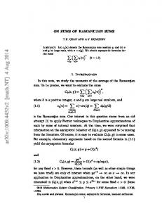
The distribution of the inferred temperatures shows a similar trend with decreasing count size for all six lakes (Figure 1). The total range and the interquartile range increase steadily from the maximum simulated count sum of 200 down to about 100 specimens. As the sample size decreases further, both continue to rise but in a more abrupt and irregular way to reach approximately twice their original size at a count sum of 50. Between a sum of 35 and 45 head capsules both statistics start to increase disproportionally, although for some lakes the range of inferred values remains remarkably constant down to a count sum of 20–25 (e.g., ENG, LOC). Both range and interquartile range at a given sample size are of the same order of magnitude for five of the six lakes. LOC, BUR, SCW, FÄL and ENG, for example, yield a total range of 1.31–1.63 °C and an interquartile range of 0.36–0.49 °C for a count sum of 100. For LÄM the inferred values are very uniform down to low count sums (e.g., a total range of 1.27 °C and interquartile range of 0.23 °C for a count of 20). This is not surprising, as LÄM has a very simple sample structure, with only four taxa present in the original sample (Table 1). Also, more than 60% of the chironomids belong to a single taxon (Tanytarsus gr. lugens), with a second reaching 24% (Chironomus gr. anthracinus; see Lotter et al., 1997). For FÄL, LÄM, LOC, SCW and ENG, the median of the inferred values is more or less constant for all sample sizes. For BUR, though, a distinct trend towards cooler inferred temperatures is apparent for low count sums.
346
Figure 1. Inferred temperatures for different count sums simulated for Le Loclat (LOC), Burgäschisee (BUR), Schwendisee (SCW), Fälensee (FÄL), Engstlensee (ENG), and Lämmerensee (LÄM). Each box plot represents the results of 100 simulations for a given count sum (see text for details). The limits of the boxes represent the first and third quartiles, whereas the whiskers encompass all values that are within 1.5 times the interquartile distance from the box. Extreme values beyond the whiskers are indicated by circles. The horizontal line in the box corresponds to the median. The reconstructed temperature (Ttot) and the sample specific root mean square error of prediction (RMSEPtot) for the original sample are given next to the box plots.
347 In order to compare the variability of the inferred temperatures with the error predicted by the chironomid-temperature calibration model, we calculated the standard deviation of all 100 simulations for a given sample size. One of the error statistics commonly used to assess the performance of calibration models is the root mean square error of prediction (RMSEP) that is calculated from the residuals between the measured and inferred values (see Birks, 1995, 1998). For a large number of samples the RMSEP approximates the standard deviation of the residuals. Here, we compare the standard deviation of the low count simulations with the error predicted by the model. We argue that, as long as the variability of the low count simulations is small in relation to the error of the model, the effect of low counts on the inferred values will be negligible, as any inferred value should only be viewed in light of the prediction error. For counts of 200 head capsules, the standard deviation of the inferred values is well below one fifth of the sample specific RMSEP of the original sample (RMSEPtot) for all six lakes (Figure 2). At a count of 100, the size of all standard deviations was still below 25% and at 50 head capsules, below 40% of the RMSEPtot. For head capsule count sums below 50 the ratio increases further, although at a different rate for
each lake. For example, for SCW the standard deviation is half the RMSEPtot at a count of 45 individuals, whereas for FÄL this threshold was only reached at 15 head capsules or less. Again, LÄM shows the smallest variability of inferred values with the standard deviation barely exceeding 40% of the RMSEPtot, even for the lowest count of 5 head capsules. Finally, we calculated the mean error of the inferred values for each lake and count sum (MEi; Figure 3). We assume that if the low head capsule counts give lower or higher inferred temperatures than samples with a higher count (i.e., they produce a systematic bias) this should be apparent in a high negative or positive MEi, irrespective of the variability of the results. The mean error is negligible for LOC and LÄM even for very low head capsule counts. ENG, FÄL, and SCW all have a tendency to infer cooler temperatures from low count samples, although even at a count sum of 30 specimens the mean inferred temperature is at most 0.26 °C colder than the inferred value of the original sample (Ttot). On the other hand, BUR shows high absolute values of MEi at count sums as high as 50 head capsules (0.5 °C) and samples of five and ten specimens have inferred temperatures that are more than 1.3 °C colder than the temperature inferred from the original count.
Figure 2. Standard deviation of inferred temperatures (SD) for different count sums in relation to the sample specific root mean square error of prediction of the original sample (RMSEPtot). Each of the six lakes is represented by a separate line (the dotted line indicates LÄM with an exceptionally low SD). The y-axis values are given as standard deviation of the inferred temperatures, divided by the root mean square error of prediction.
348
Figure 3. Mean error (ME i) of inferred temperatures for the low count simulations (see text for details). Each of the six lakes is represented by a separate line (the dashed line indicates BUR with an exceptionally large absolute MEi).
Conclusions Even though only a limited number of lakes are used for this low-count simulation and the results presented here depend strongly on the data set we used, they still provide a number of insights into the way low counts can affect quantitative temperature reconstructions: (1) Count sums of 45–50 head capsules are commonly used as a minimum count size for chironomid analysis (Hofmann, 1986). At this sample size the inferred temperature values from the low count simulations are still remarkably constant. Also, the total range and interquartile range are of a similar size as at count sums of 60–80 head capsules. This suggests that no significant increase in the reliability of the results can be obtained except by drastically increasing the minimum count sum (i.e., to about 100 or 150). For a count of 45 the standard deviation of inferred temperatures compared to the prediction error of the inference model is below 50% of the RMSEPtot in all lakes. As single inferred temperatures should generally not be taken at face value in chironomid-based temperature reconstructions and interpretation of downcore trends is usually accomplished with a robust smoothing function (e.g., Birks, 1998; Brooks & Birks, 2000), we do not consider this var-
iability to be a major cause for concern in downcore temperature reconstructions. (2) For five of the six lakes the mean bias at a cut level of 45–50 head capsules is small (absolute value < 0.25 °C). Nevertheless, the results for one lake (BUR) suggest that a serious systematic error may occur when reconstructing temperatures from samples with low counts. Using 45–50 specimens, the mean error of the BUR simulations is almost 0.5 °C and at 20 head capsules, for instance, it increases further to 0.7 °C. Therefore, temperature signals inferred from low counts only should be treated with caution. A possible way to detect if temperature extremes are due to low count sums is to combine adjacent samples to give a more reliable count size. Any systematic bias will then become apparent in the difference between inferred temperatures of the amalgamated and the low count samples. (3) The results presented here are strongly dependent on the temperature inference model and on the data set used for the low count simulations. Care should therefore be taken when extrapolating our results to other geographic regions or to chironomid-temperature inference models with a different taxonomic resolution. A minimum count of 45 seems adequate for the model we used provided that single extreme temperatures are not over-interpreted and samples are tested for the possibility of a sys-
349 tematic bias (see point 2 above). The simulation method used in this study provides a simple means of estimating the effect of low head capsule counts on the accuracy of quantitative temperature inference models. For analysts relying heavily on low head capsule sums in their interpretation, it is important to assess the effect of low counts on their temperature reconstructions. As described here, this can be done by using a number of lakes from the surface-sediment calibration data set to produce subsamples of lower count sums. Alternatively, samples from the same core material with larger count sums and a similar composition as the lowcount samples of interest can be used for the low count simulations. Finally, the simplest way of obtaining a more reliable count sum is still by processing more material or, if samples are taken contiguously, by pooling adjacent samples prior to temperature reconstruction.
Acknowledgements We thank H.J.B. Birks and S. Juggins for discussions on the use of inference models and H.J.B. Birks, I.R. Walker and an anonymous reviewer for helpful comments on the manuscript. Funding was provided by the Swiss Federal Office of Education and Science (Grant No. 97.0117) within the framework of the European Union Environment and Climate project CHILL-10,000 (Climate history as recorded by ecologically sensitive arctic and alpine lakes during the last 10,000 years: a multi-proxy approach; Contract No. ENV4-CT970642) and by the Swiss National Science Foundation within the framework of Priority Programme Environment (project 5001-044600). This is CHILL-10,000 contribution No 28.
References Birks, H. J. B., 1995. Quantitative palaeoenvironmental reconstructions. In Maddy, D. & Brew, J. S. (eds), Statistical Modelling of Quaternary Science Data. Technical Guide 5. Quaternary Research Association, Cambridge, 161–254. Birks, H. J. B., 1998. Numerical tools in palaeolimnology – progress, potentialities, and problems. J. Paleolim. 20: 307–332. Birks, H. J. B. & J. M. Line, 1992. The use of rarefaction analysis for estimating palynological richness from Quaternary pollenanalytical data. Holocene 2: 1–10. Birks, H. J. B., J. M. Line, S. Juggins, A. C. Stevenson & C. J. F. ter Braak, 1990. Diatoms and pH reconstruction. Phil. Trans. R. Soc. Lond. B 327: 263–278.
Brooks, S. J. & H. J. B. Birks, 2000. Chironomid-inferred late-glacial and early-Holocene mean July air temperatures for Krakenes Lake, western Norway. J. Paleolim. 23: 77–89. Cwynar, L. C. & A. J. Levesque, 1995. Chironomid evidence for lateglacial climatic reversals in Maine. Quat. Res. 43: 405–413. Hill, M. O., 1973. Diversity and evenness: a unifying notation and its consequences. Ecology 54: 427–432. Hofmann, W., 1986. Chironomid analysis. In Berglund, B. E. (ed.), Handbook of Palaeoecology and Palaeohydrology. John Wiley and Sons, Chichester, 715–727. Legendre, P. & L. Legendre, 1998. Numerical Ecology. Developments in Environmental Modelling 20. Elsevier, Amsterdam, 853 pp. Levesque, A. J., F. E. Mayle, I. R. Walker & L. C. Cwynar, 1993. A previously unrecognized late-glacial cold event in eastern North America. Nature 361: 623–626. Line, J. M., C. J. F. ter Braak & H. J. B. Birks, 1994. WACALIB version 3.3 – a computer program to reconstruct environmental variables from fossil assemblages by weighted averaging and to derive sample-specific errors of prediction. J. Paleolim. 10: 147–152. Lotter, A. F., H. J. B. Birks, W. Hofmann & A. Marchetto, 1997. Modern diatom, cladocera, chironomid, and chrysophyte cyst assemblages as quantitative indicators for the reconstruction of past environmental conditions in the Alps. I. Climate. J. Paleolim. 18: 395–420. Lotter, A. F., H. J. B. Birks, W. Hofmann & A. Marchetto, 1998. Modern diatom, cladocera, chironomid, and chrysophyte cyst assemblages as quantitative indicators for the reconstruction of past environmental conditions in the Alps. II. Nutrients. J. Paleolim. 19: 443–463. Maher, L. J., Jr., 1972. Nomograms for computing 0.95 confidence limits of pollen data. Rev. Palaeobot. Palynol. 13: 85–93. Mosimann, J. E., 1965. Statistical methods for the pollen analyst: multinomial and negative nomial techniques. In Kummel, B. & Raup, D. (eds), Handbook of Paleontological Techniques. Freeman, San Francisco, 636–673. Müller, B., A. F. Lotter, M. Sturm & A. Ammann, 1998. Influence of catchment quality and altitude on the water and sediment composition of 68 small lakes in Central Europe. Aquat. Sci. 60: 316–337. Olander, H., H. J. B. Birks, A. Korhola & T. Blom, 1999. An expanded calibration model for inferring lakewater and air temperatures from fossil chironomid assemblages in northern Fennoscandia. Holocene 9: 279–294. Palmer, S. L., 1998. Subfossil chironomids (Insecta: Diptera) and climatic change at high elevation lakes in the Engelmann sprucesubalpine fir zone in Southwestern British Columbia. M.Sc. Thesis, University of British Columbia, Vancouver, 105 pp. Rull, V., 1987. A note on pollen counting in palaeoecology. Pollen et Spores 29: 471–480. ter Braak, C. J. F. & S. Juggins, 1993. Weighted averaging partial least squares regression (WA-PLS): an improved method for reconstructing environmental variables from species assemblages. Hydrobiologia 269/270: 485–502. ter Braak, C. J. F., S. Juggins, H. J. B. Birks & H. van der Voet, 1993. Weighted averaging partial least squares regression (WA-PLS): definition and comparison with other methods for species-environment calibration. In Patil, G. P. & Rao, C. R. (eds), Multivariate Environmental Statistics. Elsevier Science Publishers, Amsterdam, 525–560.
350 Walker, I. R., 1987. Chironomidae (Diptera) in paleoecology. Quat. Sci. Rev. 6: 29–40. Walker, I. R., 1993. Paleolimnological biomonitoring using freshwater benthic macroinvertebrates. In Rosenberg, D. M. & Resh, V. H. (eds), Freshwater Biomonitoring and Benthic Macroinvertebrates. Chapman & Hall, New York, 306–343. Walker, I. R., R. J. Mott & J. P. Smol, 1991b. Allerød-Younger Dryas lake temperatures from midge fossils in Atlantic Canada. Science 253: 1010–1012.
Walker, I. R., S. E. Wilson & J. P. Smol, 1995. Chironomidae (Diptera): quantitative paleosalinity indicators for lakes of western Canada. Can. J. Fish. Aquat. Sci. 52: 950–960. Walker, I. R., A. J. Levesque, L. C. Cwynar & A. F. Lotter, 1998. An expanded surface-water palaeotemperature inference model for use with fossil midges from eastern Canada. J. Paleolim. 18: 165–178. Walker, I. R., J. P. Smol, D. R. Engstrom & H. J. B. Birks, 1991a. An assessment of Chironomidae as quantitative indicators of past climatic change. Can. J. Fish. Aquat. Sci. 48: 975–987.