Two-Dimensional Torus of a Hamiltonian System ..... corresponding to T5 are shown. Table 1. Linear Normal Modes around the 2-D Invariant Torus T5 in the ...
J. Nonlinear Sci. Vol. 15: pp. 159–182 (2005) DOI: 10.1007/s00332-005-0663-z
©
2005 Springer Science+Business Media, Inc.
Effective Computation of the Dynamics Around a Two-Dimensional Torus of a Hamiltonian System ` Jorba1 F. Gabern1 and A. 1
Departament de Matem`atica Aplicada i An`alisi, Universitat de Barcelona, Gran Via 585, 08007 Barcelona, Spain E-mails: {gabern,angel}@maia.ub.es
Received September 17, 2004; accepted February 9, 2005 Online publication June 13, 2005 Communicated by E. Doedel
Summary. The purpose of this paper is to give an explicit analysis of the nonlinear dynamics around a two-dimensional invariant torus of an analytic Hamiltonian system. The study is based on high-order normal form techniques and the computation of an approximated first integral around the torus. One of the main novel aspects of the current work is the implementation of the symplectic reducibility of the quasi-periodic timedependent variational equations of the torus. We illustrate the techniques in a particular example that is a quasi-periodic perturbation of the well-known Restricted Three Body Problem. The results are useful for describing the neighborhood of the triangular points of the Sun-Jupiter system. Key words. lower-dimensional tori, quasi-periodic Floquet theory, normal forms, reducibility
1. Introduction In this work we focus on numerical methods to describe the dynamics near an elliptic equilibrium point of a Hamiltonian system, under a time-dependent quasi-periodic perturbation. These methods can be applied to different physical and chemical problems where dynamical systems tools have already been shown to be of practical interest. For instance, we mention applications to mission design in astrodynamics [KLMR00], [GKL+ 04], to the study of the ionization of Rydberg atoms in molecular dynamics [UJP+ 02], and to the study of the stability of the Trojan asteroids in dynamical astronomy [GJ01] (the example we have used in this paper belongs to the latter field). One way to generalize
160
` Jorba F. Gabern and A.
the models in these autonomous examples is by considering time-dependent perturbations. In many situations, these perturbations are quasi-periodic. In this case the quasiperiodic Normal Form is a very interesting tool for studying these more sophisticated models. These procedures can also be adapted easily to compute center manifolds around a two-dimensional torus. Center manifolds, also known as Normally Hyperbolic Invariant Manifolds or NHIMs [Wig94], are prominent, for instance, in the construction of the phase space geometrical structures that mediate chemical reactions through a rank-1 saddle (see [WBW04a], [GKMR04]), and in understanding transport phenomena in Celestial Mechanics (see [GKL+ 04], [ABWF03], [WBW04b], [DJK+ 05]). Another practical example is related to ongoing work (see [GKM05]) on the motion of a spacecraft near an asteroid pair. If the model for the binary is based on a stable relative periodic orbit and the perturbation of the Sun is taken into consideration, it is possible to write the model for the spacecraft as a quasi-periodic perturbation of a relatively simple autonomous model. This model has elliptic points with the corresponding “stable” neighborhoods. These neighborhoods can be studied in detail with the techniques developed here. In particular, these tools allow us to find stable invariant tori suitable to “park” the spacecraft to do observations of the binary as the pair orbits around the Sun. There are several theoretical results dealing with quasi-periodic perturbations of a Hamiltonian system, which we mention in the following paragraphs. To simplify the reading, we skip most of the technical details and hypothesis, to only focus on the ideas. Full details are provided in the listed references. General references on Hamiltonian mechanics are [AM78], [AKN88], [Arn89], [MH92]. The effect of a quasi-periodic perturbation on an elliptic equilibrium point is considered in [JS96], [JV97b] (see also [BHJ+ 03]). There, under suitable conditions, it is shown that there exists an invariant torus replacing the elliptic point. By “replacing” we mean that the torus goes to the equilibrium point when the perturbation goes to zero. For definiteness, let d be the number of degrees of freedom of the Hamiltonian system and r the number of basic frequencies of the perturbation. Under quite general conditions, the linear dynamics around this torus can be described as the direct product of d oscillators, which come from the linear modes of the elliptic point of the unperturbed system. The nonlinear dynamics has been considered in [JV97b], [JV01], where it is shown that for each normal mode, there exists a one-parameter family of invariant tori of dimension r +1 that continues the linear mode into the complete (nonlinear) system. Due to the density of the resonances, this family is parametrized on a Cantor set of nearly full Lebesgue measure. Moreover, if we select s normal modes (1 ≤ s ≤ d), there exists a s-parametric family of tori of dimension r + s that extends the combination of the selected modes to the nonlinear system. Due to the Hamiltonian structure, the dimension of an invariant torus cannot be greater than half the dimension of phase space (this is d + r in our case). Tori of dimensions strictly lower than d + r are usually called lower-dimensional tori. The existence of lower-dimensional tori has already been considered by many authors; among them, we cite [ELi88], [Bou97], [Sev97], [Sev98]. The Lyapunov stability of a normally elliptic torus is a much more difficult topic. It is widely accepted that, if the number of degrees of freedom is larger than two, generic Hamiltonian systems do not present Lyapunov stability. This phenomenon is called Arnol’d diffusion since it was first conjectured by V. I. Arnol’d in [Arn64] (see
Nonlinear Dynamics Around a 2-Dimensional Torus
161
[AKN88] for a more general exposition). However, this diffusion is very small and it is possible to derive bounds that imply that, under quite general conditions, the time to escape from the neighborhood of a linearly stable object is extremely large (see, for instance [GDF+ 89], [PW94], [MG95], [JV97a], [Nie04]). In applications, the stability for long time intervals is called effective stability. One advantage of this approach is that, by means of numerical techniques, one can derive explicit bounds for concrete examples [Sim89], [CG91], [JV98], [GJ01]. It has been used to show, for instance, that some asteroids are effectively stable in a simplified model for the solar system [GS97]. The example selected in this work is known as Tricircular Coherent Problem (TCCP) and models the motion of an asteroid in the Sun-Jupiter system, taking into account perturbations coming from Saturn and Uranus. It is written as a three-degrees of freedom Hamiltonian system with a perturbation that depends quasi-periodically on time, with two basic frequencies, H = H0 (x, y) + ε H1 (x, y, �).
(1)
Here, H0 denotes the unperturbed system (in our case, the Restricted Three-Body Problem; see Section 1.1), H1 is the perturbation, (x, y) ∈ R3 × R3 is the configurationmomenta pair, � = (θ1 , θ2 ) ∈ T2 , θ j = ω j t + θ j(0) , j = 1, 2, and = (ω1 , ω2 ) is the vector of basic frequencies of the perturbation. Without loss of generality, the components of the vector are supposed to be linearly independent over the rationals. This example is described in more detail in Section 1.1. We focus on one of the elliptic equilibrium points of H0 . The first step in our study is the numerical computation of the 2-D torus that replaces this point in H . This torus is obtained as a truncated Fourier series with numerical coefficients. The computation is based on the approximation of an invariant curve of a suitable section of the flow by means of the methods developed in [Jor00], [CJ00], and then using the flow of the differential equation to obtain a representation of the 2-D torus by means of a Fourier series depending on � = (θ1 , θ2 ). Different approaches to computing invariant tori can be found in [DJ95], [Sim98], [ERS00], [SOV05]. Then, the linear transformation that reduces the linear variational flow around the torus to constant coefficients, the so-called quasi-periodic Floquet change, is also obtained as a numerical Fourier series. To this end, we use the method developed in [Jor01] to obtain the Floquet transformation for the invariant curve of the section, and we globalize it by means of the variational flow to produce the Floquet change for the 2-D torus. There are several procedures to do this, and the main difficulty here is to select one such that the produced change is a canonical transformation. The next step is to produce a Taylor-Fourier expansion of the Hamiltonian H around the torus, in the coordinates given by the Floquet transformation. This implies that the expansion does not contain linear terms (because the torus is invariant) and the coefficients of the quadratic part do not depend on � (because of the Floquet coordinates). Then, by means of the Lie series method, we construct the normal form of the Hamiltonian up to high order. To save computer memory, we follow the scheme given in [Jor99] to avoid the construction of the Lie triangle. Finally, we compute the changes of variables that go from the initial phase space to the normal form coordinates, and vice versa. All these computations are performed by a specific algebraic manipulator, written in C++ by the authors, that allows us to perform the required operations. This is a generalization of the code developed in [Jor99] and [GJ01].
` Jorba F. Gabern and A.
162
Using the normal form we can describe the dynamics around the torus, and the changes of variables allow us to send this information to the initial system. As this torus is normally elliptic, there exist invariant tori of dimensions 3, 4, . . ., d + 2 nearby that can easily be obtained from this normal form. Finally, we also compute an approximate first integral of the system to estimate the diffusion around the invariant torus. This allows us to derive a zone of effective stability by computing a bound on the drift of this approximate integral. From a theoretical point of view, the main novelty of this work is the method for deriving the symplectic Floquet change around an invariant torus. From a more applied point of view, we have shown how to combine numerical and analytical techniques to give a quite complete description of a neighborhood of a lower-dimensional torus of a Hamiltonian system. There are many references dealing with the numerical description of a neighborhood of a fixed point, and a few related to the vicinity of a periodic orbit (as already mentioned elsewhere in this paper). One of our goals is to show how to extend these techniques to describe a neighborhood of a lower-dimensional torus. We note that the computation of a normal form around a 2-D torus of an autonomous Hamiltonian system is different from the computations presented here. The main difference is that, in the autonomous case, the situation is far from being perturbative: The actions conjugated to the angles on the torus have to be defined in a neighborhood of the torus, and this introduces a “semiglobal” component in the construction. The same situation occurs for periodic orbits; for more details, compare [JV98] with [SGJM95] or [GJ01]. 1.1. A Model Example We will illustrate the techniques with an example from celestial mechanics, the socalled Tricircular Coherent Problem (TCCP). This is a model for the motion of a particle under the gravitational attraction of the Sun, Jupiter, Saturn and Uranus. The model is based on a (numerically computed) quasi-periodic solution of the planar Four-Body problem given by these bodies. This solution lies on an invariant 2-D torus for which a representation in Fourier series is computed explicitly. The model can be written as a quasi-periodic time-dependent perturbation, with two basic frequencies, of the wellknown Sun-Jupiter Restricted Three-Body Problem (RTBP, see [Sze67]). The motion of the particle is written in a frame where the Sun and Jupiter are fixed, respectively, at (µ, 0, 0) and (1 − µ, 0, 0). Saturn and Uranus are revolving with a motion close to circular in the (x, y) plane around the center of masses of the system. The Hamiltonian is given by HT CC P =
1 α1 (θ1 , θ2 )( px2 + p 2y + pz2 ) + α2 (θ1 , θ2 )(x px + yp y + zpz ) 2 +α3 (θ1 , θ2 )(ypx − x p y ) + α4 (θ1 , θ2 )x + α5 (θ1 , θ2 )y � � 1−µ µ m sat m ura −α6 (θ1 , θ2 ) , + + + qS qJ qsat qura
(2)
where (x, y, z) ∈ R3 are the configuration coordinates for the particle, ( px , p y , pz ) are the corresponding momenta, q S2 = (x − µ)2 + y 2 + z 2 is the square of the dis-
Nonlinear Dynamics Around a 2-Dimensional Torus
163
2 tance of the particle to the Sun, q J2 = (x − µ + 1)2 + y 2 + z 2 to Jupiter, qsat = 2 (x − α7 (θ1 , θ2 ))2 + (y − α8 (θ1 , θ2 ))2 + z 2 to Saturn, qura = (x − α9 (θ1 , θ2 ))2 + (y − α10 (θ1 , θ2 ))2 + z 2 to Uranus, θ1 = ωsat t + θ10 and θ2 = ωura t + θ20 . The concrete values of the mass parameters are µ = 9.538753600 × 10⁻⁴ , m sat = 2.855150174 × 10⁻⁴ , and m ura = 4.361228581 × 10⁻⁵ . The functions αi (θ1 , θ2 ){i=1÷10} are quasi-periodic functions that are computed by a Fourier analysis of the numerical solution of the Four Body Problem (the Sun plus three planets), and they contain the terms of the perturbation given by Saturn and Uranus. The concrete values of the frequencies are ωsat = 0.597039074021947 and ωura = 0.858425538978989. For a description of the construction of this model, as well as the concrete values of the αi (·) functions, see [GJ04] (a file with the numerical values of the Fourier coefficients can be downloaded from http://www.maia.ub.es/~gabern/).
2. Normal Form around an Invariant Torus This section discusses the details of the computation of the Floquet transformation for the torus, and the effective computation of the normal form. In what follows, we will use Taylor-Fourier expansions, with floating point coefficients, to represent the functions involved in the computations. For the examples here, the Taylor expansions are taken up to degree 16 (because of RAM memory limits) and the truncation of the Fourier series has been selected so that the representation error is of the order 10−9 . More concretely, we write a generic Taylor-Fourier polynomial as P(q, p, θ1 , θ2 ) =
N f1 N � � �
min(N f1 − j1 ,N f2 )
�
Pr,k j ei( j1 θ1 + j2 θ2 ) q k p k , 1
2
r =0 |k|=r j1 =−N f1 j2 =max( j1 −N f1 ,−N f2 )
where Pr,k j ∈ C, j = ( j1 , j2 ) ∈ Z2 , k = (k 1 , k 2 ) ∈ Zd × Zd is a multi-index (k j = �d j j j (k1 , k2 , . . . , kd ), j = 1, 2) and |k| ≡ l=1 (|kl1 | + |kl2 |). In the present work, we have used the following truncation values: N = 16, N f1 = 20, and N f2 = 10, although in some places, we use higher accuracy, as we explicitly mention in the text. This choice of the truncation values for the Fourier series guarantees the representation error stated above. This is checked numerically by comparing, for instance, the truncated series representing an invariant 2-D torus with its corresponding numerical integration. This is also discussed in Section 2.6. 2.1. The 2-D Invariant Torus That Replaces the Elliptic Fixed Point As mentioned before, the elliptic equilibrium points of (1) for ε = 0 become, under general conditions, quasi-periodic solutions with the same frequencies as the perturbation if ε belongs to a set of positive measure (for details, see [JS96], [JV97b], [BHJ+ 03]). For instance, this implies that, if the previous hypotheses hold, the elliptic triangular points L 4,5 [Sze67] of the RTBP are replaced by 2-D tori in the TCCP. For most of the values of ε, these tori are normally elliptic [BHJ+ 03].
` Jorba F. Gabern and A.
164 0.8675
-0.4975
0.867
-0.498
0.8665
-0.4985
0.866
-0.499
0.8655
-0.4995
0.865
-0.5
0.8645 -0.501
-0.5005
-0.5
-0.4995
-0.499
-0.4985
-0.498
-0.4975
-0.497
-0.5005 -0.8675
-0.867
-0.8665
-0.866
-0.8655
-0.865
-0.8645
Fig. 1. Planar projections of the 2-D invariant torus that replaces L 5 : T5 . Left: (x, y)-projection. Right: ( px , p y )-projection.
To compute this 2-D invariant torus, we have taken the section θ1 = 0 (mod 2π ) to introduce the map �
x¯ = f (x, θ ), θ¯ = θ + ω,
(3)
� � where x ∈ R2d , θ ≡ θ2 , ω = 2π ωω21 − 1 , and f can be evaluated from a numerical integration of the flow associated with (1). Using the methods described in [Jor00], [CJ00], we have computed the invariant curve of (3) that corresponds to the 2-D invariant torus that replaces L 5 in the TCCP model, with an accuracy of 10−12 . The 2-D torus is easily reconstructed using numerical integrations starting on a mesh of points on the invariant curve. Finally, a Fourier transform allows us to compute the Fourier coefficients of a parametrization with respect to the angles (θ1 , θ2 ). The (x, y) and ( px , p y ) projections of the resulting invariant torus are shown in Figure 1. From now on, we will call this 2-D torus T5 . Due to the symmetries of this problem, the same results hold for L 4 so we will only discuss the L 5 case. Applying the techniques described in [Jor01], we can see that this torus is normally elliptic, and we can obtain the three normal modes of the invariant curve. The normal modes are the frequencies of the three harmonic oscillators that describe the normal linear motion around the invariant torus. In Section 2.2, we discuss in detail the computation of these normal modes. In Table 1, the linear normal modes around the invariant curve corresponding to T5 are shown.
Table 1. Linear Normal Modes around the 2-D Invariant Torus T5 in the TCCP System j
Re (λ j )
±Im (λ j )
|λ j |
±Arg (λ j )
1 2 3
0.662315481969 -0.485204809265 -0.453781923686
0.749225067883 0.874400533546 0.891112768249
1.0 1.0 1.0
0.846891268646 2.077393707459 2.041801148412
Nonlinear Dynamics Around a 2-Dimensional Torus
165
2.2. Second-Order Normal Form In the previous section we discussed the computation of the invariant object that replaces the elliptic fixed point L 5 of the RTBP when the quasi-periodic perturbation is added. By means of a quasi-periodic time-dependent translation from the origin to this 2-D invariant torus, one can cancel the first-order terms in the Hamiltonian. Now, we will derive a linear change of variables that depends on time in a quasi-periodic way and that puts the second-degree terms of the Hamiltonian into a more convenient form. This is, essentially, the quasi-periodic Floquet transformation for the variational flow along the quasi-periodic orbit, but taking into account the symplectic structure of the problem. To simplify further steps in the normalizing process, we also apply a complexifying change of variables that puts the second-degree terms of the Hamiltonian in the so-called diagonal form. 2.2.1. The Symplectic Quasi-Periodic Floquet Change. The linear flow around the 2-D invariant torus (T5 in the example) is described by a linear system of differential equations (the variational equations) that depends quasi-periodically on time: z˙ = Q(θ1 , θ2 )z, ˙ θ1 = ω1 , θ˙2 = ω2 ,
(4)
where z ∈ R2d and Q is a real 2d × 2d matrix. Our final goal is to find a real, symplectic and quasi-periodic change of variables, z = P r (θ1 , θ2 )x, reducing (4) to a constant system with real coefficients: x˙ = Bx,
d B ≡ 0. dt
(5)
We will proceed in two steps: First, we will see that such a change of variables exists in the complex domain. As in our case the obtained complex matrix admits a real form, the second step will be to build a real change from the complex one (see [Jor01] for a concrete example where this real matrix does not exist). The entire procedure is constructive, so the implementation in a computer program will follow easily from the explanation. Reducibility in the Poincar´e section. Let us consider the θ1 = 0 (mod 2π ) section of the flow defined by (4). Then, we have the following linear quasi-periodic skew product: � z¯ = A(θ )z, (6) θ¯ = θ + ω, � � where θ ≡ θ2 and ω = 2π ωω21 − 1 (in the example, ω = 2.75080755611202) is the rotation number of the invariant curve defined by the slice θ1 = 0 (mod 2π ) of the 2-D invariant torus. Assume that (6) can be reduced to an autonomous diagonal system, y¯ = �y,
� = diag(λ1 , . . . , λ2d ),
` Jorba F. Gabern and A.
166
by means of a linear transformation z = C(θ )y. We write C(θ ) as (�1 (θ ), . . . , �2d (θ )), where � j (θ ) are the columns of C(θ ). Then it is clear that the couples (λ j , � j ) can be obtained as the eigenvalues and eigenfunctions of the following problem. A(θ )� j (θ ) = λ j � j (θ + ω),
j = 1, . . . , 2d.
(7)
This problem has been solved for the TCCP model with an accuracy of 10−12 . See [Jor01] for more details on this computation. Remark. As A(θ ) is a real matrix, if λ j and � j (θ ) satisfy (7), then λ∗j and � j∗ (θ ) also satisfy (7) (λ∗j and � j∗ (θ ) are the complex conjugates of λ j and � j (θ ), respectively). We construct the matrix C(θ ) as C(θ ) = (�1 (θ ), �2 (θ ), . . . , �d (θ ), �1∗ (θ ), �2∗ (θ ), . . . , �d∗ (θ )), where the � j are column vectors. Then, the matrix � takes the form � = diag(λ1 , λ2 , . . . , λd , λ∗1 , λ∗2 , . . . , λ∗d ). The eigenfunctions � j (θ ) are scaled in such a way that �� j �2 = 1, where �V (θ )�22 = � ∗ t � dk=1 (vk (θ�)vk+d (θ ) − vk∗ (θ )vk+d 2 , for V (θ ) = (v1 (θ ), v2 (θ ), . . . , v2d (θ )) and � (θ ))� 2 2 ilθ �α(θ )�2 = l |αl | for α(θ ) = l αl e , αl ∈ C. The Change of Variables for the Flow. The next goal is to compute a quasi-periodic change of variables z = P c (θ1 , θ2 )y that transforms the flow given by (4) into y˙ = D B y,
(8)
where D B = diag(iν1 , iν2 , . . . , iνd , −iν1 , −iν2 , . . . , −iνd ) and ν j is such that λ j = . Note that ν j is exp(iν j T1 ), where T1 is the period related to the first frequency, T1 = 2π ω1 defined modulus integer multiples of 2π . In general, we select a special value of k j ∈ Z T1 for each j = 1, 2, . . . , d such that the values of ν j are as close as possible to the ones of the RTBP. This is the natural choice from a perturbative point of view and it also allows us to obtain a symplectic transformation. Proposition 2.1. The solution of P˙ c (θ1 , θ2 ) = Q(θ1 , θ2 )P c (θ1 , θ2 ) − P c (θ1 , θ2 )D B , θ˙1 = ω1 , θ˙2 = ω2 , with initial conditions P c (0) = C(θ2(0) ), θ1 (0) = 0, θ2 (0) = θ2(0) , is the linear change of variables with complex quasi-periodic coefficients that transforms system (4) into system (8).
Nonlinear Dynamics Around a 2-Dimensional Torus
167
Proof. If we insert the change z = P c (θ1 , θ2 )y into equation (4) and if we ask whether (8) is satisfied, then P c is such that P˙ c (θ1 , θ2 ) = Q(θ1 , θ2 )P c (θ1 , θ2 ) − P c (θ1 , θ2 )D B .
(9)
On the �other hand, we integrate equation (4) from t = 0 to t = T1 with the initial condition z(0) = � j (θ2(0) ), θ1 (0) = 0, θ2 (0) = θ2(0) . Note that this is equivalent to applying A(θ2(0) ) to the vector � j (θ2(0) ). Using (7), it is easy to see that the solution of this integration, which we denote by x(t), ¯ satisfies x(T ¯ 1 ) = A(θ2(0) )� j (θ2(0) ) = λ j � j (θ2(0) + ω). An elementary result in the theory of ordinary differential equations states that if x˜1 (t) is a solution of x˙1 = Q(t)x1 , then x˜2 (t) = exp(at)x˜1 (t) is a solution of x˙1 = (Q(t) + a I )x1 , with a being any complex number. Thus, x(t) ˆ = exp(−iν j t)x(t) ¯ is a solution of P˙ c = (Q − iν j I2d )P c , j
j
� j (θ2(0) )).
with the same initial condition (x(0) ˆ = Note that it corresponds to the first three columns of equation (9). Moreover, it satisfies the following relation: x(T ˆ 1 ) = exp(−iν j Tn u)x(T ¯ 1 ) = (λ j )−1 λ j � j (θ2(0) + ω) = � j (θ2(0) + ω). Realification. In order to actually implement the Floquet change, we are interested in computing the real change of variables. Proposition 2.2. Define the (real) matrix R by taking the real and imaginary parts of the columns of matrix C. Due to the particular construction of C, the last three columns are the conjugate values of the first three: �
1 I −i Id R(θ ) = C(θ ) d . Id i Id 2 Then the solution of P˙ r (θ1 , θ2 ) = Q(θ1 , θ2 )P r (θ1 , θ2 ) − P r (θ1 , θ2 )B, θ˙1 = ω1 , θ˙2 = ω2 ,
(10)
with initial conditions P r (0) = R(θ2(0) ), θ1 (0) = 0, θ2 (0) = θ2(0) , defines a real linear quasi-periodic change of variables, z = P r (θ1 , θ2 )x, that transforms system (4) into system (5). Moreover, this change of variables is canonical.
` Jorba F. Gabern and A.
168
The real matrix B, defined as B = R −1 C D B C −1 R, does not depend on (θ1 , θ2 ) and takes the form 0 0 ··· 0 ν1 0 · · · 0 0 0 ··· 0 0 ν2 · · · 0 .. .. . .. .. . . .. . . . . . . . . . . . 0 0 ··· 0 0 0 · · · νd . B= −ν1 0 ··· 0 0 0 ··· 0 0 0 0 0 ··· 0 −ν2 · · · . .. .. .. .. . . . .. .. . . .. . . . . 0
0
· · · −νd
0
0
···
0
Proof. Define the matrix P r in the following way: P r (θ1 , θ2 ) = P c (θ1 , θ2 )C −1 (θ1 , θ2 )R(θ1 , θ2 ),
(11)
where R(θ1 , θ2 ) and C(θ1 , θ2 ) are, respectively, the extensions of the matrices R(θ ) and C(θ ). Then, we have • P r (0) is a real matrix: P r (0) = P c (0)C −1 (θ2(0) )R(θ2(0) ) = C(θ2(0) )C −1 (θ2(0) )R(θ2(0) ) = R(θ2(0) ). • If we integrate P˙r = Q P r − P r B with P r (0) = R(θ2(0) ) as an initial condition, then P r (θ1 , θ2 ) is real ∀(θ1 , θ2 ) ∈ T2 . • If we insert the relation (11) into the differential equation (10), we obtain P˙ c C −1 R + P c (C˙ −1 )R + P c C −1 R˙ = Q P c C −1 R − P c C −1 R B. By multiplying this equation on the right-hand side by the matrix R −1 C, we get P˙ c + P(C˙ −1 )C + P c C −1 R˙ R −1 C = Q P c − P c D B . This equation holds, and corresponds to equation (9), provided that P c (C˙ −1 )C + P c C −1 R˙ R −1 C = 0. It is easy to see, by using the definition of R, that this equality is true: P c (C˙ −1 )C + P c C −1 R˙ R −1 C = 0 (C˙ −1 )R + C −1 R˙ = 0 d (C −1 R) = 0. dt
⇐⇒ ⇐⇒
Finally, to ensure that the transformation is canonical, we need only to check that P r (θ1 , θ2 ) is a symplectic matrix. This can be proved (see [GJMS01b]) by extending the matrix P r to the phase space of the autonomous Hamiltonian Hext (x, y, θ1 , θ2 , pθ1 , pθ2 ) = ω1 pθ1 + ω2 pθ2 + H (x, y, θ1 , θ2 ), where (x, y) ∈ Rd × Rd , pθk is the conjugate momentum of θk and H (·) is given by equation (1).
Nonlinear Dynamics Around a 2-Dimensional Torus
169
In our example, to check the correctness of the software, we have tested numerically that P r (θ1 , θ2 ) is symplectic on a mesh of values of (θ1 , θ2 ), with an agreement of the order of the truncation of the Fourier series. If we apply this quasi-periodic change of variables, the second-degree terms of the Hamiltonian become H2r (x, y) =
1 1 1 ν1 (x12 + y12 ) + ν2 (x22 + y22 ) + ν3 (x32 + y32 ), 2 2 2
(12)
where the frequencies ν j are the normal frequencies of the torus T5 . In the TCCP system, they take the values ν1 = −0.080473064872369, ν2 = 0.996680625156409, and ν3 = 1.00006269133083. 2.2.2. Complexification. As is usual in these types of computation, we use a complexifying change of variables to bring (12) into a diagonal form. The equations of this linear and symplectic transformation are xj =
qj + i pj , √ 2
yj =
iq j + p j , √ 2
j = 1, 2, 3.
Thus, after composing the three linear symplectic changes of variables (translation of the origin to the 2-D invariant torus, quasi-periodic symplectic transformation, and complexification), the second order of the Hamiltonian takes the form H2 (q, p) = H2c (q, p) = iν1 q1 p1 + iν2 q2 p2 + iν3 q3 p3 ,
(q, p) ∈ C6 .
(13)
2.3. Expansion of the Hamiltonian To proceed with the algorithm that constructs the normal form, we need to produce a convergent Taylor-Fourier expansion of Hamiltonian (1), in the complex coordinates used to derive (13), H=
N �
Hn (q, p, θ) + R N +1 (q, p, θ ),
n=2
where Hn , n ≥ 2, denotes a homogeneous polynomial of degree n in the variables q and p, H2 (q, p, θ ) = H2 (q, p) is given by (13), and θ = (θ1 , θ2 ) ∈ T2 . To produce the expansion in our particular example, we need only to expand the terms of the potential of the TCCP Hamiltonian (2). They are of the form 1 1 =� , sl (x − xl (θ ))2 + (y − yl (θ ))2 + z 2 where (x, y, z) ∈ R3 and l stands for S (the Sun), J (Jupiter), sat (Saturn), or ura (Uranus). From the generating function of the Legendre polynomials [AS72], √
1 1 − 2σ τ +
τ2
=
∞ � n=0
Pn (σ )τ n ,
` Jorba F. Gabern and A.
170
where Pn is the Legendre polynomial of degree n; and, taking � xl (θ )x + yl (θ )y x 2 + y2 + z2 σ =� and τ = , � xl2 (θ ) + yl2 (θ ) xl2 (θ ) + yl2 (θ ) x 2 + y 2 + z 2 it is possible to expand the nonlinear terms as � n+1 ∞ ∞ � � � 2 � �n 1 1 l 2 2 2 2 x = An (x, y, z, θ) = + y + z Pn (σ ), 2 2 sl n=0 n=0 xl (θ ) + yl (θ ) where Aln denotes a homogeneous polynomial of degree n, whose coefficients are quasiperiodic functions of θ = (θ1 , θ2 ) ∈ T2 and can be computed recurrently using � � 1 n 2n + 1 l l 2 2 2 l An+1 = 2 (xl (θ)x + yl (θ )y)An − (x + y + z )An−1 , n+1 xl (θ ) + yl2 (θ ) n + 1 (14) for n ≥ 1. The recurrence can be started using the values Al0 = �
1 xl2 (θ ) + yl2 (θ )
,
Al1 =
xl (θ )x + yl (θ )y , (xl2 (θ ) + yl2 (θ ))3/2
and can be derived easily from the recurrence of the Legendre polynomials. The expansion of the Hamiltonian is implemented as follows. First, the translation to the torus T5 is composed with the Floquet transformation and the resulting affine transformation is substituted in (14). Thereafter it is not difficult to use these recurrences to obtain the expansion up to a given order. The remaining terms of the Hamiltonian, monomials of degrees 1 and 2 in (2), are easily added by simply inserting the above-mentioned affine transformation. This strategy for the expansions has already been used in several places (see, for instance, [SGJM95], [JM99], [GJMS01a], [GJMS01b], [GJ01]). On the other hand, it is also convenient to add the momenta corresponding to the angular variables. If we denote it as pθ = ( pθ1 , pθ2 ) ∈ C2 , it is possible to write the expanded Hamiltonian in complex variables as � H (q, p, θ, pθ ) = � , pθ � + H2 (q, p) + Hn (q, p, θ ), (15) n≥3
where (q, p) ∈ C2d , θ ∈ T2 , H2 (q, p) is given by (13), = (ω1 , ω2 ), and �·, ·� is the Euclidean scalar product. 2.4. Normal Form of Order Higher Than 2 The previous expansion has been obtained in coordinates such that the Hamiltonian starts at degree 2 for the spatial variables, and that degree 2 term is already in complex normal form (13).
Nonlinear Dynamics Around a 2-Dimensional Torus
171
The goal of the normalizing transformation is to eliminate the maximum number of terms of the expansion of the Hamiltonian. We basically use the Lie series method implemented as described in [Jor99], but introducing the necessary modifications in order to deal with quasi-periodic coefficients. For completeness, we describe one step of the normalizing process. Suppose that the Hamiltonian is already in normal form up to degree r − 1, H = � , pθ � + H2 (q, p) +
r −1 �
Hj (q, p) + Hr (q, p, θ ) + Hr +1 (q, p, θ) + · · · ,
j=3
� � k k k1 k2 k i( j1 θ1 + j2 θ2 ) where Hr (q, p, θ ) = |k|=r h r (θ1 , θ2 )q p , h r (θ1 , θ2 ) = j=( j1 , j2 ) h r, j e and k = (k 1 , k 2 ) ∈ Zd × Zd is a multi-index. We will make a change of variables that suppresses the maximum number of monomials and removes the dependence on θ1 and on θ2 in the terms of order r , Hr , of the Hamiltonian expansion. The canonical transformation that accomplishes this purpose is given by the following generating function: � 1 2 G r = G r (q, p, θ ) = grk (θ1 , θ2 )q k p k , |k|=r
where the coefficients are given by � h r,k j ei( j1 θ1 + j2 θ2 ) � � 2 1 j=( j1 , j2 ) i( j1 ω1 + j2 ω2 − ν, k − k ) k gr (θ1 , θ2 ) = � h r,k j ei( j1 θ1 + j2 θ2 ) i( j1 ω1 + j2 ω2 )
if k 1 �= k 2 , if k 1 = k 2 ,
j=( j1 , j2 )�=(0,0)
In general, one should check that the frequencies ω1 , ω2 , ν1 , ν2 , . . . , νd are not in resonance up to the order of the computations. Otherwise we will have a zero divisor, which implies that this resonant term cannot be eliminated. In our example, the frequencies of the normal linear oscillations around the 2-D invariant torus T5 , ν = (ν1 , ν2 , ν3 ), and the intrinsic frequencies of the system, ω1 = ωsat and ω2 = ωura , are not in resonance up to the order considered. That is, we check at every step of the process that j1 ω1 + j2 ω2 − �ν, k� �= 0, j = ( j1 , j2 ) ∈ Z2 , k ∈ Z3 \{0}, with | j| and |k| up to the orders we have worked with. Now, the new Hamiltonian H � obtained with such a generating function, H � = H + {H, G r } +
1 {{H, G r } , G r } + · · · , 2!
does not depend on the variables θ1 and θ2 up to degree r . Here, {·, ·} denotes the canonical Poisson bracket. Thus H � is in normal form up to degree r : H � = � , pθ � + H2 (q, p) +
r −1 � j=3
Hj (q, p) + Hr� (q, p) + Hr�+1 (q, p, θ ) + · · · .
` Jorba F. Gabern and A.
172
Table 2. Coefficients of the normal form, up to degree 3 in the actions for the TCCP case. The first three columns contain the exponents of the actions, and the fourth and fifth columns are the real and imaginary parts of the coefficients. Imaginary parts must be zero, but they are not due to the different accumulation errors (basically, the one that comes from the truncation of the Fourier series). k1
k2
k3
Re (h k )
Im (h k )
1 0 0 2 1 0 1 0 0 3 2 1 0 2 1 0 1 0 0
0 1 0 0 1 2 0 1 0 0 1 2 3 0 1 2 0 1 0
0 0 1 0 0 0 1 1 2 0 0 0 0 1 1 1 2 2 3
-8.0473064872368966e-02 9.9668062515640865e-01 1.0000626913308270e+00 5.6008074695424814e-01 -1.5539627415430354e-01 5.5093985824138381e-03 5.4161903856716140e-02 6.6103538676104013e-03 -3.4144388415478051e-04 1.7078141909448842e+01 2.5316327595194634e+00 1.2040309679987733e+00 -1.7159208395247699e-03 -2.0884357984263224e-01 1.3097591687221137e+00 -8.7878491487452266e-03 -3.8394291301547680e-02 -8.1852662066825860e-03 4.8084373364571027e-04
0.0000000000000000e+00 0.0000000000000000e+00 0.0000000000000000e+00 9.9022635266146223e-14 1.9737284347219547e-14 -3.4515403004164990e-16 2.6837558280952768e-15 -2.3704452239135327e-16 1.3980906058550924e-20 7.0030369427282057e-09 5.6348897124143457e-09 2.4234795726771734e-10 8.2745567480971449e-12 2.7145888846396389e-10 8.5687025776165656e-11 1.1230163355821964e-12 4.9155879462758908e-12 2.9493958070531223e-13 4.1626694220605631e-14
After making these changes up to a suitable degree n = N , the Hamiltonian takes the form H = � , pθ � + N (q1 p1 , q2 p2 , . . . , qd pd ) + R(q, p, θ1 , θ2 ),
(16)
where N denotes the normal form (which depends only on the products q j p j ) and R is the remainder (of order greater than N ). Finally, we write the normal form N in real action-angle coordinates. This can be achieved easily by using the canonical transformation, q j = I j1/2 exp(iϕ j ),
p j = −i I j1/2 exp(−iϕ j ),
j = 1, 2, . . . , d.
It is not difficult to see that N , in these coordinates, does not depend on the angles ϕ j but only on the actions I j , N =
[N /2] � |k|=1
h k I1k1 I2k2 . . . Idkd ,
k ∈ Zd ,
h k ∈ R.
(17)
Values for the coefficients h k up to order N = 6 for our particular case of the TCCP system can be found in Table 2. As has been mentioned before, these computations have been performed up to order N = 16.
Nonlinear Dynamics Around a 2-Dimensional Torus
173
2.5. Changes of Variables We have also computed explicit expressions for the transformation from the initial variables of (1) to the normal form variables and its inverse. As usual, these changes of variables can be written as a truncated Taylor-Fourier series, with the same truncation values as the Hamiltonian. They will be used to send information from the normal form coordinates to the initial ones, and vice versa. 2.6. Local Nonlinear Dynamics Close enough to the 2-D invariant torus that replaces the equilibrium point, the nonlinear dynamics can be described accurately by the truncated normal form (17). As this is an integrable normal form, the dynamics is very simple: The phase space is completely foliated by a d-parametric family of invariant tori, parametrized by the actions I . On each torus I = I0 , there is a linear flow with a given frequency �(I0 ). If these frequencies are linearly independent over the rationals, then the torus I = I0 is filled densely by any trajectory starting on it. If the frequencies are linearly dependent over the rationals, then the orbits on this torus are not dense: If there are �i independent frequencies, the torus I = I0 contains a (d − �i )-parametric family of �i dimensional tori, each one being densely filled by any trajectory starting on it. These tori of dimension �i are the lower dimensional tori, while the tori of dimension d are the maximal dimensional ones. The diffusion due to the remainder has been studied widely in the literature (see [GDF+ 89], [Sim89], [JV98], [GJ01] and references therein), so we will omit further discussion of this topic. As we want to use the tori of the normal form as approximations to invariant tori for the complete system, we need a procedure to estimate their accuracy. One possibility is to estimate the size of the remainder (see, for instance, [JV98] or [GJ01]), but here we have chosen a more straightforward approach: Given a torus in normal form, we can tabulate an orbit on it, send this table to the coordinates of the initial Hamiltonian (2), and check if each point is obtained from a numerical integration of the previous one. The integration time is taken equal to 0.1, because we do not want the integration error to interfere with the test. For tori sufficiently close to the origin of the normal form, this test is passed within an accuracy of the same order as the truncation of the Fourier series, that is, 10−9 . All the tori displayed in this section have passed this test. Therefore, we can easily compute lower and maximal invariant tori using the truncated normal form and send them, via the change of variables, to the initial coordinates of the system. This change of variables adds two additional frequencies (the system’s intrinsic frequencies, ω1 and ω2 ) to the invariant tori. Figures 2 through 7 are examples of these computations for the TCCP system. More concretely, Figures 2 and 3 are obtained by setting I1 = I2 = 0 and I3 = I3(0) in (17), for some (small) value I3(0) > 0. This is a periodic Lyapunov orbit of the autonomous normal form N in (16) that corresponds to a three-dimensional torus for the initial Hamiltonian (2). This 3-D torus belongs to the Lyapunov family of the 2-D torus T5 (see [JV97b]), and their normal frequencies are ∂N (0, 0, I3(0) ), j = 1, 2, where N ∂ Ij is taken from (17). Figures 4 and 5 have been obtained in a similar way, but setting I2 = I3 = 0, I1 = I1(0) , and I1 = I3 = 0, I2 = I2(0) , respectively. In the coordinates
` Jorba F. Gabern and A.
174 0.8675
0.04
0.867
0.03 0.02
0.8665
0.01 0.866 0 0.8655 -0.01 0.865
-0.02
0.8645
-0.03
0.864 -0.501 -0.5005
-0.5
-0.4995 -0.499 -0.4985 -0.498 -0.4975 -0.497
-0.04 -0.04
-0.03
-0.02
-0.01
0
0.01
0.02
0.03
0.04
Fig. 2. Projection on the (x, y) (left) and on the (z, pz ) (right) planes of an elliptic threedimensional invariant torus near T5 . The intrinsic frequencies are ωsat , ωura , and ν3 = 1.000062350. The normal ones are ν1 = −0.08044599352 and ν2 = 0.9966839283. This invariant torus is generated by setting I1(0) = I2(0) = 0 and I3(0) = 0.0005.
of the initial Hamiltonian (2), these two tori are contained in the plane z = pz = 0. Figure 6 displays two projections of a four-dimensional invariant torus near T5 . Finally, in Figure 7, two different projections of a five-dimensional invariant torus are shown. These graphs have been obtained computing 10,000 points on a single orbit on the torus, with a time step of 0.1 units. See the captions for more details. We note that, in this way, it is also possible to compute quasi-periodic orbits with a prescribed set of frequencies �0 , provided that �0 belongs to the domain where the normal form is accurate. The procedure is based on solving the equation ∇N (I ) = �0 by means of, for instance, a Newton method.
0.04 0.03 0.02 0.01 0 -0.01 -0.02 -0.03 -0.04 0.8675 0.867 0.8665 0.866 -0.501 -0.5005 0.8655 -0.5 -0.4995 0.865 -0.499 -0.4985 0.8645 -0.498 -0.4975 -0.4970.864
Fig. 3. Projection on the configuration space of the three-dimensional invariant torus shown in Figure 2.
Nonlinear Dynamics Around a 2-Dimensional Torus
0.885
-0.85
0.88
-0.855
0.875
-0.86
0.87
-0.865
0.865
-0.87
0.86
-0.875
0.855
-0.88
0.85 -0.53
-0.52
-0.51
-0.5
-0.49
-0.48
-0.47
-0.885 0.85
175
0.855
0.86
0.865
0.87
0.875
0.88
0.885
Fig. 4. Projections on the (x, y) (left) and (y, px ) (right) planes of an elliptic three-dimensional invariant torus. The intrinsic frequencies are ωsat , ωura , and ν1 = −0.08046185813, and the normal ones are ν2 = 0.9966790714, and ν3 = 1.000063233. This invariant torus is generated by setting I2(0) = I3(0) = 0 and I1(0) = 0.00001.
0.885
-0.485
0.88
-0.49
0.875 -0.495 0.87 -0.5 0.865 -0.505 0.86 -0.51
0.855
0.85 -0.515 -0.52 -0.515 -0.51 -0.505 -0.5 -0.495 -0.49 -0.485 -0.48 -0.475 -0.88
-0.875
-0.87
-0.865
-0.86
-0.855
-0.85
Fig. 5. Projections on the (x, y) (left) and ( px , p y ) (right) planes of an elliptic three-dimensional torus. The intrinsic frequencies are ωsat , ωura , and ν2 = 0.9966811761, and the normal ones are ν1 = −0.08048083167 and ν3 = 1.000063022. This invariant torus is generated by setting I1(0) = I3(0) = 0 and I2(0) = 0.00005.
0.015
0.015
0.01
0.01
0.005
0.005
0
0
-0.005
-0.005
-0.01
-0.01
-0.015
-0.015
0.885
-0.485
0.88 0.875 -0.52
-0.515
-0.51
-0.505
0.87 0.865 -0.5
-0.495
-0.49
-0.485
0.86 0.855 -0.48
-0.4750.85
-0.49 -0.495 -0.88
-0.875
-0.87
-0.865
-0.5 -0.505 -0.86
-0.855
-0.51 -0.85-0.515
Fig. 6. Projections on the (x, y, z) (left) and ( px , p y , pz ) (right) spaces of a four-dimensional torus near T5 . The intrinsic frequencies are ωsat , ωura , ν2 = 0.9966811761, and ν3 = 1.000063022, and the normal one is ν1 = −0.08048083168. This invariant torus is generated by setting I1(0) = 0, I2(0) = 0.00005 and I3(0) = 0.0001.
` Jorba F. Gabern and A.
176 0.9
0.015
0.89
0.01
0.88 0.005 0.87 0 0.86 -0.005 0.85 -0.01
0.84
0.83 -0.015 -0.55 -0.54 -0.53 -0.52 -0.51 -0.5 -0.49 -0.48 -0.47 -0.46 -0.45 -0.015
-0.01
-0.005
0
0.005
0.01
0.015
Fig. 7. Projections on the (x, y) (left) and (z, pz ) (right) planes of a five-dimensional torus near T5 . The frequencies are ωsat , ωura , ν1 = −0.08046420047, ν2 = 0.9966802858, and ν3 = 1.000063496. This invariant torus is generated by setting I1(0) = 0.00001, I2(0) = 0.00005, and I3(0) = 0.0001.
3. Approximate First Integral of the Initial Hamiltonian A first integral of a Hamiltonian system H (q, p, θ ) is a function F(q, p, θ ) that is constant on each orbit of the system. Functions having a small drift along the orbits are usually called “approximate first integrals” or “quasi-integrals” [GG78], [Mar80]. One of the main applications of approximate first integrals is to bound the rate of diffusion in certain regions of the phase space [CG91], [GJ01]. 3.1. Computing a Quasi-Integral It is not difficult to see that, if F(q, p, θ ) is a first integral, then {H, F} = 0.
(18)
Here we will try to solve this equation by expanding H and F in Taylor-Fourier series, in the same coordinates used to obtain (15). That is, we suppose that H is expanded in complex coordinates, as in the normal form up to degree 2. Let us write F as a truncated Fourier-Taylor expansion, F(q, p, θ1 , θ2 ) =
N �
Fn (q, p, θ1 , θ2 ),
n=2
where, as usual, Fn stands for a homogeneous polynomial of degree n in the variables (q, p), with coefficients that are truncated Fourier series in the angles θ1 and θ2 : � � � � 1 2 Fn (q, p, θ1 , θ2 ) = f n,k j ei( j1 θ1 + j2 θ2 ) q k p k . |k|=n j=( j1 , j2 )
To compute the coefficients of this expansion, f n,k j ∈ C, we solve equation (18) order by order. It is easy to see that there is some freedom while selecting the degree 2 of F, F2 . As our final goal is to bound the diffusion using this quasi-integral, a good choice is
Nonlinear Dynamics Around a 2-Dimensional Torus
177
(see [GJ01]) F2 = i
d �
qj pj .
j=1
With this choice, the Hessian of the realification of F at the origin is a positive-definite matrix. This implies that, near the origin, the level curves of F are compact surfaces. As for higher degrees, n > 2, it is possible to obtain f n,k j recursively, k icn, j
� �, j1 ω1 + j2 ω2 − k 2 − k 1 , ν
f n,k j =
k where ν = (ν1 , ν2 , . . . , νd ) and cn, j can be computed from the expansion of the Hamiltonian and the previously computed coefficients of F. During the computations, two conditions must be verified at every step of the process:
(a) ω1 , ω2 , and ν must satisfy that j1 ω1 + j2 ω2 − �k, ν� �= 0, ∀ ( j1 , j2 ) ∈ Z2 ,
∀ k ∈ Zd
such that | j| + |k| �= 0,
k (b) if j1 = j2 = 0 and k 1 = k 2 , the value cn, j must vanish.
The first is the same nonresonance condition needed for the normal form computation and it depends only on the normal and internal frequencies of the torus. The second condition has to be checked before the computation of each Fj . In our example, this second condition is satisfied in all the cases. For a discussion of condition (b), see [CG91]. In the model example, we have used the recurrence relation to compute the approximate first integral truncated at order N = 16. 3.2. Bounding the Diffusion As F is not an exact first integral, the variation of the values of F on a given trajectory of the Hamiltonian is not exactly zero. The variation can be written, in terms of the Hamiltonian expanded in real coordinates H (x, y, θ, pθ ) and in terms of the realified quasi-integral F(x, y, θ ), as F˙ = {F(x, y, θ ), H (x, y, θ, pθ )} , where (x, y) ∈ Rd × Rd and, as usual, pθ = ( pθ1 , pθ2 ) are the momenta corresponding to the angles θ = (θ1 , θ2 ) ∈ T2 . Then it is easy to see that the diffusion can be estimated by bounding the following expansion: F˙ =
N �� n>N l=3
{Fl , Hn−l+2 } +
�
{F2 , Hn } .
n>N
We will use the same procedure as in [GJ01]. Thus, we use lemmas in [GJ01] and [CG91] to estimate the size of the terms of the Hamiltonian that have not been numerically
` Jorba F. Gabern and A.
178
computed, i.e., those homogeneous polynomials with degree greater than N . The norms appearing in the lemmas should be modified in order to deal with two angles, but it is easy to see that the lemmas are still valid. A bound for the drift of the formal first integral F is obtained by means of the following: � be integers such that 3 ≤ N ≤ N � and Lemma 3.1. Let N and N �, �Hk � ≤ Sk , 3≤k≤N k−� N +1 � �Hk � ≤ h E, k > N , �Fk � ≤ Q k , 3 ≤ k ≤ N. Then, if hρ < 1,
˙ ρ ≤ R(ρ), � F�
where R(ρ) =
N −2 �
( j + 2)ρ j Q j+2
j=1
+
N −2 �
� N